| Issue |
A&A
Volume 553, May 2013
|
|
|---|---|---|
| Article Number | A78 | |
| Number of page(s) | 24 | |
| Section | Extragalactic astronomy | |
| DOI | https://doi.org/10.1051/0004-6361/201220286 | |
| Published online | 07 May 2013 | |
Online material
Appendix A: Spectroscopic success rate in the VVDS-Wide fields
We computed the spectroscopic success rate (SSR) in the VVDS-Wide 14 h and 22 h fields
for a given redshift range by following the prescriptions in Ilbert et al. (2006): we compared the number of galaxies with flag =
4, 3 and 2 over the total number of galaxies (those with flag = 4, 3, 2, 1 and 0).
Because flag = 1 galaxies have a 50% reliability and no redshift information is
available for flag = 0 galaxies, we took advantage of the latest photometric redshifts
from CFHTLS survey to estimate the number of galaxies with flag = 1 and 0 that belong to
the redhsift range of interest. With the previous steps we estimate the SSR in the 22 h
field as  (A.1)where
N22 h,spec(zr)
is the number of galaxies with flag = 4, 3 and 2 in the redshift range
zr, and
N22 h,phot(zr)
is the number of galaxies with flag = 1 and 0, and with a photometric redshift in the
same redshift range. As the available imaging data in the 14 h eld is not as deep as the
CFHTLS, we show in the following that we can assume that the SSR in the 14 h field
follows the same distribution as in the 22 h field, for which CFHTLS photometry is
available.
(A.1)where
N22 h,spec(zr)
is the number of galaxies with flag = 4, 3 and 2 in the redshift range
zr, and
N22 h,phot(zr)
is the number of galaxies with flag = 1 and 0, and with a photometric redshift in the
same redshift range. As the available imaging data in the 14 h eld is not as deep as the
CFHTLS, we show in the following that we can assume that the SSR in the 14 h field
follows the same distribution as in the 22 h field, for which CFHTLS photometry is
available.
First we checked the properties of the stars in these two VVDS-Wide fields. The fraction of stars in the 22 h (14 h) field is 66% (51%) for flag = 4 sources, 38% (26%) for flag = 3 sources, 24% (23%) for flag = 2 sources, and 11% (12%) for flag = 1 sources. So the fraction of stars is similar in both fields for flag = 2 and 1 sources, while higher in the 22 h field for flag = 4 and 3. We checked that the normalised distributions of the VVDS-Wide stars as a function of their observed IAB-band magnitude in both fields are similar for each flag. We note that stars with high confidence flag are brighter than the low confidence ones, as expected. The fraction of bright stars (IAB ≤ 21) in the 22 h (14 h) field is 75% (67%) for flag = 4 stars, 49% (43%) for flag = 3 stars, 30% (29%) for flag = 2 stars, and 19% (16%) for flag = 1 stars. These fractions suggest that there is a higher density of bright stars in the 22 h area than in the 14 h one, that translates in a higher fraction of stars for flag = 4 and 3 sources, while faint stars have similar densities in both fields, leading to a similar fraction of stars with flag = 2 and 1. Because of this, we assumed that the fraction of stars among flag = 0 sources, that we estimate in the 22 h field from the CFHTLS photometry, is similar in 22 h and 14 h fields.
The distribution of galaxies at z ≥ 0.9, the redshift range in which
we are interested on, are also similar in both fields. Because of this, we assumed that
the photometric distribution of galaxies with flag = 1 and 0 is similar in both fields,
and we use those in 22 h field to estimate
N14 h,phot and the SSR in the 14 h
field:  (A.2)where
n14 h(1,0) is the total number of
sources (galaxies and stars) with flag = 1 and 0 in the 14 h field, and
f22 h(zr) = N22 h,phot(zr)/n22 h(1,0)
is the fraction of sources with a photometric redshift in the redshift range
zr over the total population of sources with flag = 1 and
0 in the 22 h field.
(A.2)where
n14 h(1,0) is the total number of
sources (galaxies and stars) with flag = 1 and 0 in the 14 h field, and
f22 h(zr) = N22 h,phot(zr)/n22 h(1,0)
is the fraction of sources with a photometric redshift in the redshift range
zr over the total population of sources with flag = 1 and
0 in the 22 h field.
Appendix B: GALFIT residual images of blended MASSIV close pairs
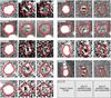 |
Fig. B.1
Original i-band image (left panels) and residual images from the GALFIT fit with one (central panels) and two components (right panels) of those MASSIV close pair candidates with overlapping components in the kinematical maps. The grey scale has been chosen to enhance the light residuals in the images. The solid contour marks the targeted MASSIV source to guide the eye. The ID of the showed MASSIV source is labelled in each left panel. |
| Open with DEXTER | |
In this Appendix we detail the modelling in the i band of those MASSIV close pair candidates with overlapping components in the kinematical maps. We used GALFIT v3.0 (Peng et al. 2010) to model the light distribution with two independent Sérsic components. We set the initial positions of the sources using the information from the kinematical maps, and we did not impose any constraint on the other initial parameters of the fit (i.e., luminosity, effective radius, Sérsic index, position angle and inclination). Because of the minimisation process preformed by GALFIT in the fitting, the best model with two components should not be unique and the convergence to a given solution should depend on the initial values of the parameters defined by the user. We checked, by exploring randomly the space of initial values, that the number of good solutions is at most two. Where two good solutions exist, the one that better reproduces both the velocity field and the velocity dispersion map is preferred. To illustrate the need of a second component to describe the blended close pair systems in MASSIV, we show in Fig. B.1 the original image in the i band and the residual image from GALFIT with one and two components. In all the cases the residual map from the one component fit suggests that a second component is present. This Figure also demonstrates that both the seeing (~0.7″) and the depth of the i-band images used in the present study are good enough to characterise sources with two overlapping components.
Appendix C: Completeness of the close pair sample
Throughout the present paper we have assumed that the close pair systems detected in the MASSIV sample are representative for galaxies with IAB ≤ 23.9. The MASSIV sample comprises galaxies fainter than this luminosity limit, and in this Appendix we justify the boundary applied in our analysis.
The VVDS parent samples of the MASSIV sample are randomly selected in the IAB band (Le Fèvre et al. 2005). Because of this, we studied the distribution of MASSIV sources as a function of the IAB-band magnitude to obtain clues about the completeness of the MASSIV sample in our close pair study. We show the cumulative distribution of all MASSIV sources and of those with a close companion (both major and no major) in the top panel of Fig. C.1. Obviously, we are able to detect single MASSIV galaxies at fainter magnitudes than the close pairs (IAB = 24.4 vs. 23.8) because in the latter case we have to detect both the principal source and the companion galaxy, which is usually fainter.
Lets assume for a moment that the detection curve of the MASSIV sources is a step function that is 1 for IAB ≤ IAB,lim and 0 for fainter magnitudes. In this ideal case, IAB,lim is defined by the fainter galaxy (close pair) detected. Thus, we should only be able to detect close pairs at IAB ≤ 23.8, and the measured merger fraction in the total MASSIV sample (IAB ≤ 24.4) will be lower than the real merger fraction because of the missing faint close pairs with IAB > 23.8. Of course, the detection curve in the MASSIV sample is more complicated than a step function, and could depend on redshift, geometry, luminosity, etc. Instead of trying to estimate the detection curve for MASSIV sources and for close companions to recover statistically the missing close pairs (see Patton et al. 2000; de Ravel et al. 2009, for examples of this kind of correction), we define the IAB-band magnitude up to which the detected close pairs are representative of the total MASSIV sample, named IAB,comp, and in our study we only keep those sources brighter than IAB,comp to ensure reliable merger fractions.
The MASSIV sample is a representative subsample of the global star-forming population (Contini et al. 2012), and we expect the MASSIV galaxy pairs to be also a random sample of this global population. Therefore, the distributions in the IAB band of the total and the close pair MASSIV sources should be similar when the close pairs detection was slightly affected by incompleteness issues. Following this idea, we performed a Kolmogorov-Smirnov (KS) test over the total and close pair MASSIV galaxies with IAB ≤ IAB,lim, and explored different values of IAB,lim, from 23.0 to 24.5. Then, the completeness magnitude IAB,comp was defined by the minimum in the KS estimator D, i.e., where both distributions have the lower probability to be different. This exercise provides the curve in the bottom panel of Fig. C.1, that states IAB,comp = 23.9. We repeated this procedure with the major merger sample, and we obtain a similar distribution of D values, reinforcing our choice.
In summary, in the estimation of the merger fraction we only use those MASSIV galaxies with IAB ≤ IAB,comp = 23.9. This ensures that the close pair sample is a random subsample of the total MASSIV one, and we avoid any bias related with the shallower detection curve of close pairs compared with that of the total MASSIV sample.
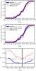 |
Fig. C.1
Top: cumulative distribution in the apparent IAB magnitude of the total MASSIV sample (green line), the close pair sample (red line) and the total MASSIV sample with IAB ≤ 23.9 (blue line). Middle: the same than before, but the red line shows the distribution of the major merger sample. Bottom: Kolmogorov-Smirnov estimator D of the total MASSIV sample distribution against the close pair (blue solid line) and the major merger (red dashed line) distributions. We computed D for those galaxies brighter than a given IAB magnitude. The solid (dashed) horizontal line marks the minimum in the D distribution for close pairs (major mergers). The vertical solid line marks the IAB magnitude at the minimum value of D, IAB,comp = 23.9. |
| Open with DEXTER | |
© ESO, 2013
Current usage metrics show cumulative count of Article Views (full-text article views including HTML views, PDF and ePub downloads, according to the available data) and Abstracts Views on Vision4Press platform.
Data correspond to usage on the plateform after 2015. The current usage metrics is available 48-96 hours after online publication and is updated daily on week days.
Initial download of the metrics may take a while.