| Issue |
A&A
Volume 552, April 2013
|
|
|---|---|---|
| Article Number | A116 | |
| Number of page(s) | 17 | |
| Section | Interstellar and circumstellar matter | |
| DOI | https://doi.org/10.1051/0004-6361/201220807 | |
| Published online | 11 April 2013 | |
Online material
Appendix A: Code tests and details
Our code is designed to treat the excitation of rotational CO levels and other simple molecules in a variety of conditions actually present in the analysis of astronomical observations (Sect. 1). We therefore focus our tests on the validity of the calculations in these cases. It is well known that in quite extreme cases, such as very opaque molecular transitions (particularly of HCO+, van Zadelhoff et al. 2002), the line formation is very difficult to treat and predictions can significantly vary when different codes are used. The treatment of these cases is strongly dependent on the numerical treatment of the line profile, the discretization in cells, etc. Even worse, the results dramatically depend on the properties of the discussed object (size of the cloud, variations of the physical conditions across it, etc.), which in actual cases are not well known. In this context, when opacities are so high, the observational parameters do not practically depend on the properties of the inner regions, but just on the (very complex) structure of a very thin cloud “photosphere”, a surface layer that can hardly be adequately described. We therefore focus on tests that request difficult convergence and accurate calculations, but avoid extreme, hardly useful cases.
A.1. 1D models
We first compared the results from our code with previously published calculations of well-tested codes in 1D cases. For this purpose, we used the 1D version of the program. For comparison, we used calculations published by Lucas (1976) and Bernes (1979), who used well-known codes and applied them to CO emission in spherical collapsing clouds. The Bernes code is a Monte Carlo approach that has been extended to other molecules and a variety of physical conditions and is very widely used today. The code by Lucas is based on a discrete treatment of the frequencies and directions that approximates the derivatives by finite (very small) differences and the integrals by quadrature forms. To compare results from both papers with our calculations, some interpretation of the assumptions and approaches in these papers is necessary.
We first reproduce the calculations by Lucas (1976). We chose as an example the CO J = 2–1 and J = 1–0 profiles calculated for his low-density case and outer velocity equal to 1 km s-1. The local velocity dispersion (1-σ) is equal to 1 km s-1. This is the most representative case, since the level populations are not thermalized and the profile shows a clear self-absorption due to the excitation variation across the cloud. In this case the (constant) physical conditions are density n = 103 cm-3, temperature T = 30 K and CO relative abundance X(CO) = 10-4. We suppose that the published profile is given in units of Rayleigh-Jeans-equivalent temperature (otherwise it is difficult to understand that the 2–1 line, mostly thermalized and opaque, shows this low peak temperature) and that the background cosmic continuum was subtracted from the published profile; both choices are common when predictions are to be compared with radioastronomical observations.
We also assumed that the collisional rates used by Lucas (1976) are those published by Green & Thaddeus (1976; the Lucas paper was published when these calculations were still in press). We took only the downward collisions from Green & Thaddeus, the excitation rates were calculated following the microreversibility principle (Sect. 2), but we are not sure that the same was done by Lucas. Finally, we calculated the collisions for the gas temperature, 30 K, by interpolating those published for 20 K and 40 K.
Following all these recipes, we resolved the excitation state of the CO levels and calculated the resulting J = 1–0 and J = 2–1 profiles, which are shown in Fig. A.1. We checked that convergence is reached in the several parameters used in the code (number of cells, number of considered rays, etc; see Sects. 2.2 and A.2). Clearly, the profiles are identical to those given by Lucas (1976) up to the accuracy that the comparison with the published profiles allows, despite the uncertainties and possible sources of error that remain in the comparison of both codes. We therefore consider the test satisfactory.
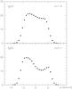 |
Fig. A.1
Predicted profiles obtained with our code for the 12CO J = 1−0 and J = 2−1 lines, for the physical conditions used by Lucas 1976 (the case with density of 103 cm-3 and a maximum radial velocity of 1 km s-1), to be compared with profiles in Figs. 1 and 2 of Lucas (1976). |
| Open with DEXTER | |
The comparison with calculations by Bernes is more complete because this author also published the distribution of the excitation temperature. The model nebula is somewhat larger (with a radius of 3 × 1018 cm instead of 1018 cm). Other parameters are n = 2 × 103 cm-3, T = 20 K, and X(CO) = 5 × 10⁻⁵. The velocity field is the same as in Lucas (1976); we assume that the local velocity broadening used by Bernes is also a 1-σ dispersion. We also applied the microreversibility principle in calculating the collisional rates.
The predicted profile and excitation temperature (Tex) for the CO J = 2–1 transition derived with our code are shown in Figs. A.2 and A.3, to be compared with the corresponding figures in Bernes (1979). We assume that Bernes (1979) gives the profile in units of brightness temperature, in view of the zero-level (equal to about 2.7 K) and because the profile peak is equal to the kinetic temperature (as expected in thermalized and opaque lines). Clearly, our results are identical to those obtained by Bernes, within the uncertainties, including the numerical noise that is not negligible in the Monte Carlo approach.
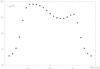 |
Fig. A.2
Predicted profile obtained with our code for the 12CO J = 2−1 line, for the physical conditions used by Bernes (1979), to be compared with the corresponding profile in his Fig. 3. |
| Open with DEXTER | |
 |
Fig. A.3
Predicted excitation temperature obtained with our code for the 12CO J = 2−1 line for the physical conditions used by Bernes (1979), to be compared with his Fig. 2. The green, open squares represent the kinetic temperature of the cells. |
| Open with DEXTER | |
We note that these two examples are very demanding tests for the treatment of radiative transfer and its effects on the molecular level excitation (the key problem), close to the too complex and scarcely practical problems discussed before. The opacities are high, of about 50, and therefore the interaction between different points in the nebula is very complex and the iterative process becomes slow. The differences found between our calculations and those of the previous codes are ~1% (often indistinguishable from the figures); the largest difference, ~3%, was found in the comparison with the excitation temperature of J = 1–0 predicted by Bernes (1979) for the outermost boundary of his model cloud (outer 1017 cm, where complex population cascades lead to some increase of the 1–0 excitation). We verified that differences found in various runs of our code with different values of the numerical parameters are smaller than 1%; we show in Sect. A.2 that in some cases our code may show a numerical noise of about 1% in excitation temperature, which could also appear in the calculations shown here, although it does not obviously manifest itself when different runs are compared. Most probably the main differences with respect to previous works are due to our interpretation of the previous calculations.
Differences of a few percent have often been found when very different codes were compared, see Bernes (1979) and van Zadelhoff et al. (2002). Their origin, except for the numerical noise in Monte Carlo calculations, is difficult to know, as concluded by the quoted authors.
The fact that the tests of our 1D code are positive convincingly shows that it treats the problem correctly.
A.2. Comparison between 1D and 2D codes
We have mentioned (Sect. 2) that our code easily evolves to a 2D treatment, since, in some way, the two dimensions are included in the code structure. We therefore built a 2D code in which axial symmetry is assumed and the cells are defined in terms of distance to the axis of symmetry and to the equator. We assumed symmetry with respect to the equator in the examples we show here, but it is not necessary in the code (when this symmetry is assumed only one half the cells are needed).
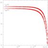 |
Fig. A.4
Comparison between the excitation temperature (Tex) and the equivalent radiation temperature (Trad) of the J = 2−1 transition calculated with the 1D version of the code (continuous and dashed lines) and with the 2D version (red, empty squares). Calculations performed for the same model as for Fig. A.3 (from Bernes 1979). |
| Open with DEXTER | |
The tests of the 2D code were performed running the 2D code with the same conditions as assumed in the 1D examples. In other words, the cell definition and radiative transfer treatment were performed fully in 2 dimensions, with their coordinates given by the distances to the axis and equator, but the physical conditions in the cloud satisfy spherical symmetry. In this way, the 2D treatment can be checked by comparing it with 1D code results, whose accuracy was discussed above (Sect. A.1). A few non-local 2D calculations of CO excitation have been published for cases similar to those we are interested in, e.g. Hogerheijde & van der Tak (2000), but the lack of details on the calculation and nebula model prevents a careful comparison. These authors also checked their code by comparing its CO predictions with the 1D results from Bernes (1979).
In Fig. A.4 we compare the predictions of the excitation temperature of the CO J = 2–1 transition derived from our 1D code (continuous black line) and those from the 2D code (open red squares). We used the same nebula model as in Sect. A.1 to compare our results with those by Bernes (1979), including the collisional rates. We considered a total of 40 cells in the 1D calculations and 900 cells in the 2D case. We also show in this figure the equivalent temperature of the radiation field (Trad) seen in each cell (lower discontinuous, black line and red squares); of course, the excitation temperature is placed between this radiation field temperature and the kinetic one (20 K), its value is given by the collisional/radiative de-excitation probability ratio.
The comparison is again very positive. We can see some numerical errors (differences in excitation temperatures for cells at the same distance to the center, between different cells of the 2D code and with respect to the 1D calculations), but they are very moderate, ≲1%. The errors in Tex are comparable to those found for Trad, and calculating the radiation intensity in just one point per cell is probably the source of the whole uncertainty.
We also performed calculations for conditions under which the errors may be slightly larger. When the macroscopic velocity field becomes higher, the velocity variations within a given cell can be relatively large. In such cases, errors may appear in the calculation of the relative velocities of two cells, resulting in errors in the calculations of the emission and absorption rates at the relevant frequencies.
In Fig. A.5 we show the excitation and radiation temperatures for the same case as before but increasing the maximum velocity to 4 km s-1. For calculations in the upper panel, we took 40 and 100 cells for the 1D and the 2D models respectively (symbols are the same as in Fig. A.4). As we see, differences slightly higher than 1% are noticeable in the 2D calculations and with respect to the 1D results. Even some systematic underexcitation of the 1D calculations can be seen in the figure. As mentioned, the reason for the appearance of some numerical noise is that the cells are relatively large (which is particularly the case of the spherical cells). The results converge for higher numbers of cells, as we can see in Fig. A.5, lower panel, for which we used 75 and 900 cells for the 1D and 2D cases. In this panel we also show 1D calculations using more recent collisional rates (pointed, green line), taken from the LAMBDA-database2 (Wernli et al. 2006). As we see, the results are different from those using calculations by Green & Thaddeus (1976), as in our previous runs, but not dramatically, by about 5% in Tex. From now on, we use these more accurate rates in our tests. We finally show still more recent calculations from the same database (Yang et al. 2010), dash-point line; the differences are still smaller, ≲2%, showing the moderate changes in the final calculations often found when new collisional rates are incorporated.
For higher values of the macroscopic velocity, convergence becomes increasingly difficult. As we show below, in these cases calculating the level populations with the well-known LVG approximation is much more efficient.
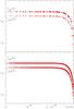 |
Fig. A.5
Calculations similar to those performed for Fig. A.4, but for a model cloud in which the highest inward velocity is equal to 4 km s-1. Upper panel: using 40 and 100 cells for the 1D and 2D calculations. Lower panel: using 75 and 900 cells; the green point and dash-point lines represent 1D calculations when more recent collisional rates are used (see text). Note the improvement in the calculation noise when more cells are used and the moderate influence of collisional rates. |
| Open with DEXTER | |
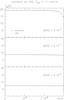 |
Fig. A.6
Comparison between calculations performed using our non-local treatment of radiative transfer (squares) and the LVG approximation for a cloud model similar to that used previously (from Bernes 1979) for different values of the relative CO abundance (which led to an optically thin case for X(CO) = 5 × 10⁻⁹, lower panel). The green dotted lines represent a modification of the LVG approach trying to simulate boundary effects. |
| Open with DEXTER | |
A.3. Comparison with LVG calculations
The well-known LVG approximation holds when in a cloud the module of the macroscopic velocity increases monotonically with radius, with a gradient steep enough to ensure that points decoupled radiatively are still close and expected to show similar physical and excitation conditions. As mentioned in Sect. 2, the averaged radiation intensity in any point, which rules the radiatively stimulated rates in the transitions, is then a local parameter and the treatment becomes equivalent to the definition of an escape probability of photons, which represents the percentage of photons emitted by the gas that actually escapes from the cloud in spite of self-absorption (trapping). LVG codes are therefore very fast and relatively simple, though they incorporate the main ingredients of the problem. It is also known that this approximation yields reasonable values of the level population even when the conditions are only marginally satisfied (although the resulting line profile must in any case be calculated by solving the exact radiative transfer equation for the derived level populations). Because of the inherent radiative decoupling introduced by the LVG approximation, it can easily be extended to 2- or even 3D calculations, the (local) excitation being in fact independent of the geometry of the cloud at large scale.
We performed LVG calculations for the nebula models we studied in the previous subsections and other similar ones. In the LVG approximation, the effects of the nebula size and macroscopic velocity field enter the calculation of the opacity via the factor r/V, τ ∝ r/V, where r and V are the distance to the center and the expansion or collapse velocity at this distance; the local velocity dispersion is neglected. Since we will apply this treatment to cases in which the local velocity is not negligible compared to the macroscopic one, we substituted in our calculations the value of V by V + ΔV/2, where ΔV is the width at half-maximum of the local velocity dispersion.
In a first case, we considered the same nebula model as Bernes (1979), see Sect. A.2. We recall that this time we did not use the collisional rates by Green & Thaddeus but the more recent calculations (Sect. A.3). In Fig. A.6, upper panel, we compare results from our non-local ’exact’ treatment (black squares) with those from the LVG approximation (red dashed line). The LVG results are surprisingly similar to those from the non-local code, even if the highest macroscopic velocity is just comparable to the local dispersion. In reality, the LVG predictions are independent of the point of the nebula we are considering, because in this nebula model the value of r/V is constant. Therefore, in the outer regions, where very little photon trapping occurs because we are very close to the nebula boundary, the non-local code gives a somewhat lower excitation (approaching the values obtained for lower abundances, see below) and the LVG limit of very low local velocity dispersion cannot deal with this effect. It is possible to define “equivalent” values of r to simulate this effect in the LVG code and improve the predictions in outer regions. We do not discuss these procedures here, but just show (pointed green lines) calculations in which we took for the outer points an equivalent radius of the cloud equal to the distance between the point and the outer circumference in the direction perpendicular to the radius direction between the point and the cloud center; we point out that the results are somewhat improved in the outer regions but not yet fully satisfactory.
In the other panels of the figure, we show the same calculations for lower values of the CO relative abundance, and therefore of the opacities. As expected, the excitation temperature decreases (because of the less frequent trapping) and the agreement with LVG improves (because in the optically thin limit the statistical equilibrium equations, which give the level populations, become independent of the radiative transfer treatment).
We have seen that when the local and macroscopic velocities are practically the same, far from the LVG assumptions of negligible local ΔV, the predictions of the simple LVG codes are very reasonable. Only the decreasing excitation toward the edge of the cloud in very opaque cases can hardly be accounted for by an LVG treatment, and therefore the asymmetries of the profiles seen in Sect. A.1 cannot be obtained from it.
 |
Fig. A.7
Comparison between calculations performed using our non-local treatment of radiative transfer (squares) and the LVG approximation, similar to those of Fig. A.6, except for a higher value of the outer collapse velocity, in this case equal to –4 km s-1. The very low opacity case is identical to that of Fig. A.6 (lowest panel) and is not displayed again. |
| Open with DEXTER | |
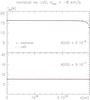 |
Fig. A.8
Same as Fig. A.7 but for an outer collapse velocity of –8 km s-1. |
| Open with DEXTER | |
We performed calculations in other cases. In Figs. A.7 and A.8, we can see the same model but assuming a higher outer collapse velocity Vout of –4 and –8 km s-1. As expected, the LVG predictions are still better. Again, for lower opacities the coincidence is absolute.
 |
Fig. A.9
Same as Fig. A.7 but without the macroscopic velocity field. |
| Open with DEXTER | |
We also repeated the calculations for the case where the macroscopic velocity is equal to zero, Fig. A.9, and the LVG approach is forced to maximum. (As said before, in this case the local velocity dispersion in fact substitutes the macroscopic velocity in our LVG calculations.) For high optical depths (high abundance) the agreement is good, because the line is practically thermalized (and, of course, the agreement is very good for very low opacities). But for cases with moderate opacities, where the radiative transfer effects are relevant, there is a significant difference between the non-local and LVG codes; in any case, the difference is not extreme, only of about 20% in terms of Tex(2−1), a value that could be improved if we changed the definition of the LVG-equivalent velocity.
 |
Fig. A.10
Same as Fig. 7 but assuming a slowly increasing macroscopic velocity, defined by a constant logarithmic gradient of the velocity of 0.1. |
| Open with DEXTER | |
We also performed a calculation similar to our standard case (Bernes nebula model), but with a slowly increasing value of the radial velocity (Fig. A.10). This is particularly interesting for studying AGB circumstellar envelopes, which present a velocity law of this kind. We considered a law V(r) = Vout × (r/Rout)ϵ. A constant logarithmic velocity gradient was chosen because this is the parameter that actually enters the calculation of the LVG escape probability. We took a quite extreme case with ϵ = 0.1. In a law of this kind, the variation of the velocity along the radial direction is slow and all spherical layers interact radiatively in that direction (not in the tangential one). Results in Fig. A.10 show a good behavior of the LVG approach, except for the very outer regions. Here r/V is not constant across the nebula.
Finally, we performed calculations for higher-J transitions with our non-local code and compered them with LVG results. We show here as an example calculations of the J = 6−5 excitation for our standard cloud model (from Bernes 1979), but for variable CO abundances and with ten rotational levels. (We verified that the results for J = 2−1 in these calculations are almost identical to those previously reported with only six rotational levels.) We show the results in Fig. A.11. Except for the edge effects in the very optically thick case, the LVG results are identical to those from the non-local treatment. The excitation temperature increases close to the cloud edge in the non-local calculations for high abundance, which is because transitions below J = 6−5 are very opaque and those above it are optically thin and, therefore, photon cascades tend to relatively overpopulate levels with J ~ 6 in the outer layers. This test is very demanding, because the opacity is very high for J = 5–4 and lower transitions but the excitation state is low for high-J levels (the energy of the J = 6 level is 116 K but the kinetic temperature in the model is just 20 K). The comparable excitation given by the non-local and LVG calculations confirms the accuracy of our calculations also for high-J levels and even for strong underexcitation. Similar tests are difficult to perform by comparison with previous works because of the lack calculations for these high transitions.
 |
Fig. A.11
Same as Fig. A.6 but for transition J = 6−5 and including a total of ten rotational levels. |
| Open with DEXTER | |
In summary, we have seen that the LVG approximation is quite accurate in producing the excitation conditions of molecular gas for clouds showing radial velocities, even if they are very low and the conditions of the approximations are in fact not satisfied. The good agreement of our calculations with the LVG ones in all reasonable cases must also be considered as an independent test of our non-local code.
A.4. Axisymmetric nebulae
We applied our 2D code to clouds with axial, but without spherical symmetry. In all cases discussed here, we assumed symmetry with respect to the equatorial plane. We considered as basic example the same physical conditions as in previous subsections, i.e., the Bernes (1979) nebula model with constant density, temperature, and CO abundance (n = 2 × 103 cm-3, T = 20 K, X(CO) = 5 × 10⁻⁵), and radial velocity increasing linearly up to a value of 1 km s-1 in the nebula limit. One of the radii (equatorial or axial) is kept equal to 3 × 1018 cm and the other is decreased to 1018 cm. The result is a strongly prolate or oblate structure, in which the velocity gradients are different in the equatorial and axial directions (while the final velocities are the same).
We show the resulting Tex(2–1) in Figs. A.12 and A.13 (red squares), continuous red lines join points along the equator and along the axis. For comparison we show the results from the spherical cases with cloud radii of 1018 and 3 × 1018 cm (continuous black lines); as expected, the prolate and oblate structures show intermediate excitations between these two extreme cases. The points with the lowest values of Tex are always close to the edge.
 |
Fig. A.12
Red squares: 2D calculations of the J = 2−1 excitation temperature performed for a model cloud similar to that discussed previously (the Bernes model cloud) but showing a strongly prolate structure. The red lines join points along the axis (those reaching higher values of the distance to the center, r) and along the equator. Continuous black lines: calculations for spherical clouds with radii equal to the maximum and minimum radius of the prolate cloud. |
| Open with DEXTER | |
 |
Fig. A.13
Red squares: 2D calculations of the J = 2−1 excitation temperature performed for a model similar to that of Fig. A.12 but now showing a strongly oblate structure. The red lines join points along the equator (those reaching higher values of the distance to the center, r) and along the axis. Continuous black lines: calculations for spherical clouds with radii equal to the maximum and minimum radius of the prolate cloud. |
| Open with DEXTER | |
Finally, we incorporated Keplerian rotation in our code (which is our goal in order to apply it to rotating disks). We considered rotation around the symmetry axis in our oblate structure (as defined above) and the rotation velocity was assumed to vary inversely with the square-root of the distance to the axis, with a velocity of 0.3 km s-1 in the outer regions, and reaching values higher than 4 km s-1 in the innermost code cells. (This field would correspond to rotation around a central compact mass of a few solar masses, but does not really represent a stable Keplerian movement, because the total mass of the cloud is already larger than this value.) The results can be seen in Fig. A.14; again we represent the J = 2–1 excitation temperatures derived for the rotating cloud and for our standard spherical clouds (continuous black lines), as in Figs. A.11 and A.12.
We recall that to facilitate the comparison with previous figures, we have assumed constant density. That is usually not the case in actual rotating disks; when we assume the density to increase toward the center (with 1/r or 1/r2), the excitation is high in the central regions and the J = 2–1 line thermalizes in them.
We also represent in Fig. A.14 predictions from our LVG code (dashed red line). For these calculations, we took the absolute values of the distance to the center and of the tangential velocity to calculate the factor r/V (as discussed in Sects. A.3, including the correction to the velocity due to the local dispersion) and ϵ = 1. Evidently, the LVG results give a rough idea of the expected excitation temperatures, but errors can be very large in this case (larger than 30%), even if we just compare the LVG results with the non-local predictions for points along the equator (squares joined by the upper red line). The reason is that in rotating clouds radiative interaction between very distant points can take place, in a complex long-distance interaction pattern, and the LVG approximation is not valid at all. Particularly in inner points, where rotation is fast, the LVG procedure implies that radiative interaction only takes place within a very small region, though in reality even line radiation from the edges of the cloud can be absorbed in these innermost layers.
In summary, the LVG calculations have been found to give a good representation of the molecular excitation in spherical and axisymmetric clouds showing radial velocity fields, even in extreme conditions (including the case without a macroscpic velocity field). However, in a rotating cloud the LVG results only give an idea of the true Tex values, particularly in the inner regions that are in fast rotation. It is difficult to imagine how the standard LVG formalism could be modified to obtain a better approximation to the radiative transfer in this case.
 |
Fig. A.14
Red squares: calculations similar to those shown in Fig. A.13 but assuming that the oblate structure is in Keplerian rotation. The dashed red line represents LVG calculations for the distance and absolute value of the velocity used here, which do not approximate the “exact” code results. |
| Open with DEXTER | |
Appendix B: Line predictions for alternative models of the Red Rectangle
We investigated the variations of the predicted intensity of the lines discussed here as a function of the physical conditions in the disk, notably of the gas temperature, which is the parameter discussed in more detail in this paper. In Sect. 4.1, we have already presented the line intensity variation if we include a central region (at a distance to the axis smaller than 2 × 1015 cm) with temperature and density higher than in our standard model by a factor 2. Figure 2 showed that this new component can help to explain the high line-wing emission in intermediate-J transitions, but yields too strong emission in the J = 16−15 line, therefore the problem of the too high line-wing intensity persists. We present here a similar case, in which the values of T(Rkep) are the same as in our standard model, but we increase the slope of the dependence of T with the distance to the center from 1 to 1.3. This is equivalent to an increase in the temperature by 20% at the point R = Rkep/2 and by 50% at 2 × 1015 cm from the star. Results are shown in Fig. B.1. Clearly, the predicted intensity for the J = 16−15 transitions is already too high and this new law leads to a significant increase in the J = 6−5 line wings. As discussed in Sect. 4.1, models of rotating disks of this kind cannot explain the J = 6−5 line wings and the J = 16−15 profile.
 |
Fig. B.1
Profiles of the observed mm- and submm-wave transitions (black) and the predictions of our code (red points), assuming that the slope of the temperature profiles increases to 1.3 instead of 1, as in our standard model, Fig. 1, Table 2. The symbols have the same meaning as in Fig. 1; note the values of the multiplicative parameter. |
| Open with DEXTER | |
We investigated the deviations of the predictions from the observed profiles assuming changes in the temperature from our best-fitting model. In Figs. B.2 and B.3, we show predictions assuming that the temperature varies by ± 20% with respect to our standard model, while the rest of the parameters remain the same. These variations are sufficient to yield predictions incompatible with the data (though not by a very large factor), taking the calibration uncertainties into account, and can be considered in these conditions as a measure of the uncertainty in the estimated temperature values.
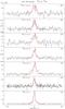 |
Fig. B.2
Profiles of the observed mm- and submm-wave transitions (black) and the predictions of our code (red points), assuming that the temperature increases by 20% with respect to our standard model, Fig. 1, Table 2. The symbols have the same meaning as in Fig. 1; note the values of the multiplicative parameter. |
| Open with DEXTER | |
 |
Fig. B.3
Profiles of the observed mm- and submm-wave transitions (black) and the predictions of our code (red points), assuming that the temperature decreases by 20% with respect to our standard model, Fig. 1, Table 2. The symbols have the same meaning as in Fig. 1; note the values of the multiplicative parameter. |
| Open with DEXTER | |
The low-J transitions depend very little on the kinetic temperature for the investigated cases.
Finally, we considered a nebula model in which both the density and temperature vary. We assumed that the density increases by a factor 2 and at the same time that the temperatures decreases
by a 30%. The results are very similar to those shown in Fig. B.3, the comparison with the observations is not acceptable, but now for a variation in the temperature of a 30%. We conclude that allowing variations in the density relaxes the uncertainties in determining the temperature, but not by a large factor, from 20% to 30% in this case. Deeper changes in the model would contradict our initial intention of keeping the nebula model deduced from mm-wave maps (Bujarrabal et al. 2005) invariable as far as possible.
© ESO, 2013
Current usage metrics show cumulative count of Article Views (full-text article views including HTML views, PDF and ePub downloads, according to the available data) and Abstracts Views on Vision4Press platform.
Data correspond to usage on the plateform after 2015. The current usage metrics is available 48-96 hours after online publication and is updated daily on week days.
Initial download of the metrics may take a while.