| Issue |
A&A
Volume 551, March 2013
|
|
|---|---|---|
| Article Number | A39 | |
| Number of page(s) | 14 | |
| Section | The Sun | |
| DOI | https://doi.org/10.1051/0004-6361/201220617 | |
| Published online | 18 February 2013 | |
Online material
Appendix A: Derivation of kink mode equation
We give a short derivation of the basic equations, starting from Eqs. (3)–(5). The solutions are obtained in the three regions, inside the flux tube, outside the flux tube and in the transition layer.
A.1. Internal solution
Using the thin tube (or long wavelength) limit, the internal solutions can be
expressed as 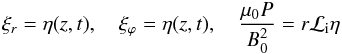 (A.1)Hence, at
r = R − l/2 = R(1 − ϵ/2),
we have
(A.1)Hence, at
r = R − l/2 = R(1 − ϵ/2),
we have 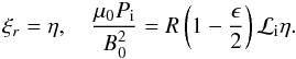 (A.2)
(A.2)
A.2. External solution
Again using the thin tube limit, we have
 (A.3)Hence, at
r = R + l/2 = R(1 + ϵ/2),
we have
(A.3)Hence, at
r = R + l/2 = R(1 + ϵ/2),
we have 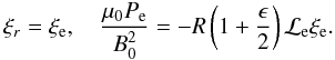 (A.4)Since both
ξr and P are
continuous across the transition layer as ϵ → 0, we can state
ξe = η + δξr, Pe = Pi + δP,
where both δξr and
δP tend to zero as ϵ → 0. Using (A.4), we have, correct to
O(ϵ2),
(A.4)Since both
ξr and P are
continuous across the transition layer as ϵ → 0, we can state
ξe = η + δξr, Pe = Pi + δP,
where both δξr and
δP tend to zero as ϵ → 0. Using (A.4), we have, correct to
O(ϵ2), 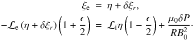 (A.5)Rearranging
Eq. (A.5), the final equation for
the propagating kink mode is
(A.5)Rearranging
Eq. (A.5), the final equation for
the propagating kink mode is 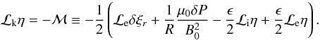 (A.6)Note that the
right hand side of (A.6) is of
O(ϵ). It is the leading order expressions for
δξr and
δP that we now need to calculate and this is done from the
transition layer solutions.
(A.6)Note that the
right hand side of (A.6) is of
O(ϵ). It is the leading order expressions for
δξr and
δP that we now need to calculate and this is done from the
transition layer solutions.
A.3. Transition layer solution
Integrating Eq. (3) across the thin
transition layer, we have 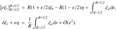 (A.7)Integrating
(4) we have
(A.7)Integrating
(4) we have
 (A.8)Remembering that
η is independent of r,
(A.8)Remembering that
η is independent of r,
 is l times
the average value of the operator ℒ and, for the linear density profile, the average
is ℒk, thus,
is l times
the average value of the operator ℒ and, for the linear density profile, the average
is ℒk, thus, 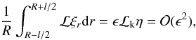 (A.9)since
ℒkη = O(ϵ). Hence, for
the linear density profile
(A.9)since
ℒkη = O(ϵ). Hence, for
the linear density profile 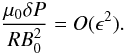 (A.10)
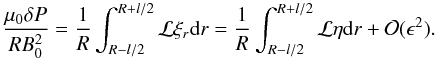
We substitute Eq. (A.7) into
Eq. (A.6) and, using both Eq. (A.10),
ℒi + ℒe = 2ℒk and that again
ℒkη = O(ϵ), this
results in the propagating kink mode equation 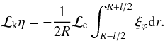 (A.11)
A.4. Integration of ξϕ across the transition layer
In this section we evaluate
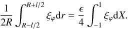 (A.12)Using the solution
for ξϕ given by (26), the integral across the transition
layer is made up of four terms. These are evaluated in turn.
(A.12)Using the solution
for ξϕ given by (26), the integral across the transition
layer is made up of four terms. These are evaluated in turn.
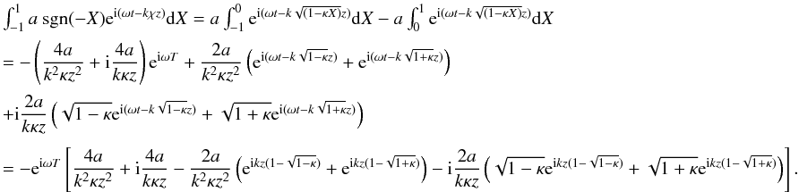
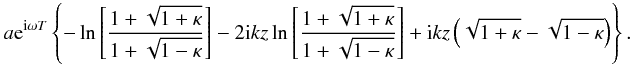
A.4.1. Term 1
Now the integral of the first term on the RHS of Eq. (26), due to the radial profile of the driving boundary condition
of ξϕ, is
 For
large kz, this is proportional to
(kz)-1. The influence of the choice of boundary
condition does becomes less important after several wavelengths.
For
large kz, this is proportional to
(kz)-1. The influence of the choice of boundary
condition does becomes less important after several wavelengths.
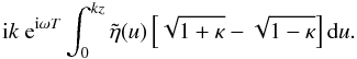
For small values of kz, we can expand the result in a series to
show that the first term is 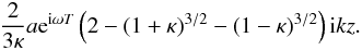 For small
κ, Term 1 can be expressed as
For small
κ, Term 1 can be expressed as
 where we have
defined
where we have
defined 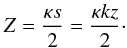 (A.13)
A.4.2. Term 2
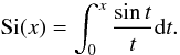
The second term on the RHS integrates to give 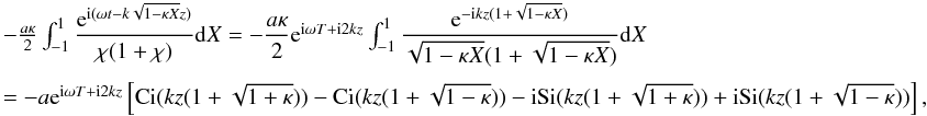 where
Ci(x) and Si(x) are the Cosine integral
and Sine integral respectively, defined by
where
Ci(x) and Si(x) are the Cosine integral
and Sine integral respectively, defined by
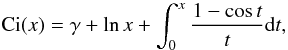
where γ = 0.57721... is Euler’s constant and
 Again this term is
proportional to (kz)-1 for large kz.
Again this term is
proportional to (kz)-1 for large kz.
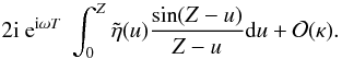
For small values of kz, it is easier to start from the integral
expression. Hence, the first two terms in the Taylor series are
 For
small values of κ, term 2 can be shown to reduce to
For
small values of κ, term 2 can be shown to reduce to
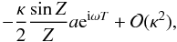 where
Z = κkz/2, as above.
where
Z = κkz/2, as above.
A.4.3. Term 3
The third term is 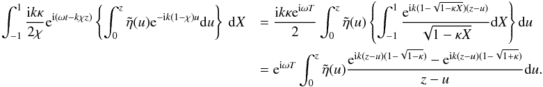 The
expansion of the coefficient of
The
expansion of the coefficient of  for small kz gives to leading order
 The expansion for
small κ gives, where
Z = κkz/2,
The expansion for
small κ gives, where
Z = κkz/2,
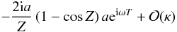
A.4.4. Term 4
Consider the final term, 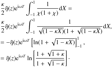 The
expansion for small κ gives
The
expansion for small κ gives 
A.5. Final expression
We can now bring together the expressions for all four terms to rewrite the kink mode
equation, (A.11), as
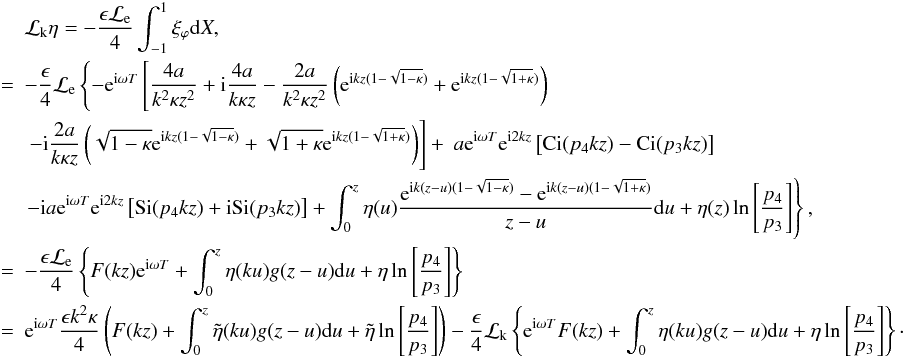 Expressing
η as
Expressing
η as  , our
final equation is
, our
final equation is  (A.14)where
 ,
,
 ,
ℒ1 = d2/dz2 − 2ikd/dz
and
ℒe = −k2κ + ℒk.
In Eq. (A.14), the operator,
ℒ1, acting on the final terms in the curly brackets on the right hand
side, results in terms that are small for κ ≪ 1. In fact, the terms
remain small even for κ ≤ 1/2. Hence, we will
neglect them and the comparison with the numerical results confirms this is a valid
assumption (see Sect. 5).
,
ℒ1 = d2/dz2 − 2ikd/dz
and
ℒe = −k2κ + ℒk.
In Eq. (A.14), the operator,
ℒ1, acting on the final terms in the curly brackets on the right hand
side, results in terms that are small for κ ≪ 1. In fact, the terms
remain small even for κ ≤ 1/2. Hence, we will
neglect them and the comparison with the numerical results confirms this is a valid
assumption (see Sect. 5).
Equation (A.14) is an inhomogeneous,
integro-differential equation for  ,
the slowly varying amplitude function that describes the damping of the kink mode.
,
the slowly varying amplitude function that describes the damping of the kink mode.
© ESO, 2013
Current usage metrics show cumulative count of Article Views (full-text article views including HTML views, PDF and ePub downloads, according to the available data) and Abstracts Views on Vision4Press platform.
Data correspond to usage on the plateform after 2015. The current usage metrics is available 48-96 hours after online publication and is updated daily on week days.
Initial download of the metrics may take a while.