| Issue |
A&A
Volume 551, March 2013
|
|
|---|---|---|
| Article Number | A39 | |
| Number of page(s) | 14 | |
| Section | The Sun | |
| DOI | https://doi.org/10.1051/0004-6361/201220617 | |
| Published online | 18 February 2013 | |
Damping of kink waves by mode coupling
I. Analytical treatment⋆
1
School of Mathematics and Statistics, University of St
Andrews,
St Andrews,
KY16 9SS
UK
2
Solar Physics and Space Plasma Research Centre (SP2RC), University
of Sheffield, Sheffield, S3
7RH, UK
3
Departament de Física, Universitat de les Illes
Balears, 07122
Palma de Mallorca,
Spain
e-mail: This email address is being protected from spambots. You need JavaScript enabled to view it.
Received:
24
October
2012
Accepted:
2
January
2013
Abstract
Aims. We investigate the spatial damping of propagating kink waves in an inhomogeneous plasma. In the limit of a thin tube surrounded by a thin transition layer, an analytical formulation for kink waves driven in from the bottom boundary of the corona is presented.
Methods. The spatial form for the damping of the kink mode was investigated using various analytical approximations. When the density ratio between the internal density and the external density is not too large, a simple differential-integral equation was used. Approximate analytical solutions to this equation are presented.
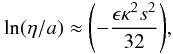
Results. For the first time, the form of the spatial damping of the kink mode is shown analytically to be Gaussian in nature near the driven boundary. For several wavelengths, the amplitude of the kink mode is proportional to (1 + exp(-z2/Lg2))/2, where Lg2 = 16/ϵκ2k2. Although the actual value of 16 in Lg depends on the particular form of the driver, this form is very general and its dependence on the other parameters does not change. For large distances, the damping profile appears to be roughly linear exponential decay. This is shown analytically by a series expansion when the inhomogeneous layer width is small enough.
Key words: magnetohydrodynamics (MHD) / Sun: atmosphere / Sun: corona / Sun: magnetic topology / Sun: oscillations / waves
Appendix A is available in electronic form at http://www.aanda.org
© ESO, 2013
1. Introduction
Coronal multi-channel polarimeter (CoMP) observations have revealed periodic Doppler shift oscillations propagating along large, off-limb coronal loops (Tomczyk et al. 2007; Tomczyk & McIntosh 2009). From the analysis of the ratio of outward and inward propagating power along loop structures, Tomczyk & McIntosh (2009) found a strong decay in the wave amplitudes as they travelled along the loop. Indeed, only shorter loops show evidence of inward power, implying the presence of either very efficient dissipation or mode conversion. Furthermore, McIntosh et al. (2011) demonstrated that these propagating, transverse loop displacements carry a significant amount of energy and hence could potentially play an important role in coronal heating (Parnell & De Moortel 2012) and/or the solar wind acceleration (Ofman 2010). Finally, the ubiquitous nature of these waves makes them very attractive as a potential seismological tool (De Moortel & Nakariakov 2012). Similar transverse oscillations have also been reported in spicules (De Pontieu et al. 2007; He et al. 2009), X-ray jets (Cirtain et al. 2007) and prominence fibrils (Okamoto et al. 2007).
The observed waves show clear, periodic variations in Doppler shifts (velocities) but only very weak signatures in intensity. This incompressible nature, together with the fact that the observed speeds are generally of the order of the local Alfvén speed gives the waves a distinct Alfvénic character (Goossens et al. 2009). Motivated by the numerous observations of waves in coronal loops, for example in Tomczyk et al. (2007), we recently performed a series of 3D numerical simulations (Pascoe et al. 2010; 2011; 2012). Using 3D simulations of loop displacements, Pascoe et al. (2010) clarified the nature of the observed loop displacements as coupled kink-Alfvén waves: transverse footpoint motions travel along the loop and through the inhomogeneity at the loop boundary, couple efficiently to (azimuthal) Alfvén waves. This mode coupling takes place at locations where phase speed of the propagating kink mode matches the local Alfvén speed (Allan & Wright 2000) and energy is transferred from the transverse kink modes to the Alfvén modes in the shell regions of the loop. Hence, the kink modes are effectively a moving source of Alfvén waves until all energy is transferred into the Alfvén waves. Pascoe et al. (2010) showed that this coupling is sufficiently efficient to qualitatively explain the observed rapid amplitude decay. This mode coupling takes place even for modest density contrasts or an arbitrary inhomogeneous medium (Pascoe et al. 2011). Further evidence for the occurence of the mode coupling presence can be found in the frequency filtering which is inherent to this mechanism. Indeed, Terradas et al. (2010) demonstrated that the damping of the transverse motions through mode coupling is frequency-dependent, with higher frequencies leading to shorter damping lengths. Subsequently, Verth et al. (2010) found evidence for this frequency in the CoMP data of Tomczyk & McIntosh (2009), strengthening the interpretation of the observed, propagating Doppler shift oscillations as coupled kink-Alfvén waves. Additional effects such as the presence of a background flow or gravitational stratification on the mode coupling mechanism were studied by Soler et al. (2011a,b).
The damping lengths obtained through mode coupling do not only depend on the frequency of the footpoint displacements but also on the width of the inhomogeneous layer at the edge of the loop. Wider layers lead to more efficient mode coupling and, hence, shorter damping lengths. The periods observed by Tomczyk et al. (2007) are of the order of several minutes (peaking at about 5 min) and to achieve the observed strong damping in this period range, a relatively wide layer, of the order of half of the loop radius, is required (Pascoe et al. 2010, 2012). Similar evidence for loops with wide boundary layers was obtained by seismological estimates derived from the damping rate of standing, kink mode oscillations by Goossens et al. (2002). Similar to the mode coupling mechanism described by Pascoe and co-authors, which operated on open flux tubes, standing, kink mode oscillations, on closed field lines, also undergo efficient damping through resonant absorption in the presence of an inhomogeneous shell region (e.g. Hollweg & Yang 1988; Goossens et al. 1992; Ruderman & Roberts 2002).
The numerical simulations of Pascoe et al. (2012) revealed a change in the characteristic damping profile of the transverse velocity displacements: at low distance, a Gaussian profile of the form exp(−z2) is present, followed by an exponential damping profile of the form exp(−z) at larger distances. The distance at which this transition between the two damping profiles occurs appears to depend on the density profile. For narrow inhomogeneous layers, the exponential damping profile is evident after only a few wavelengths. However, for wider shell regions, the damping profile is largely Gaussian except at large distances. As observational evidence (both for propagating and standing kink mode oscillations) suggests the presence of wide inhomogeneous shell regions, Pascoe et al. (2012) suggested the Gaussian profile might be best suited to the observed CoMP data. A transition to the exponential damping regime would still occur at larger distances but, due to the strong damping, the amplitudes of the Doppler shift oscillations are expected to be too small to be observationally relevant.
A related study for the time dependent evolution of a standing kink mode has been undertaken by Ruderman & Terradas (2012). They find that the temporal behaviour of the kink mode amplitude is damped in a Gaussian manner for small times, before approaching a linear exponential damping for large times.
In this paper, we investigate the mode coupling process analytically to clarify the nature of the Gaussian damping profile. The paper is organised as follows. The analytical problem is formulated in Sect. 2, followed by the derivation of the governing equations in Sect. 3. The nature of the damping profile is investigated in Sect. 4 by using various approximations. The key point of this section is to demonstrate when previously used approximations are valid and when they fail. These approximations are compared with numerical simulations in Sect. 5. Conclusions are presented in Sect. 6.
2. Problem formulation
We consider the propagation of kink waves in a semi-infinite magnetic tube. In cylindrical
coordinates r, ϕ, z with the
z-axis coinciding with the tube axis, the tube is situated in the
half-space z > 0. The equilibrium magnetic field is
in the z-direction,
B0 = (0,0,B0),
and homogeneous. The equilibrium density, ρ(r)is given by
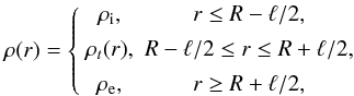 (1)where
ρi and ρe are constants, and
ρi > ρe.
Thus, the Alfvén speed,
(1)where
ρi and ρe are constants, and
ρi > ρe.
Thus, the Alfvén speed, 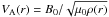 ,
is a function of radius alone and we use the notation
,
is a function of radius alone and we use the notation 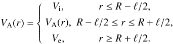 (2)The
tube is excited by imposing a velocity perturbation at z = 0. Thus, waves
are excited and these propagate into the system, namely
z > 0. We select the external Alfvén speed to be
1 Mm s-1. Distances are measured in mm and periods in seconds.
(2)The
tube is excited by imposing a velocity perturbation at z = 0. Thus, waves
are excited and these propagate into the system, namely
z > 0. We select the external Alfvén speed to be
1 Mm s-1. Distances are measured in mm and periods in seconds.
To demonstrate the Gaussian nature of the damping analytically, we neglect stratification, field line curvature and expansion of the magnetic tube. The importance of these physical phenomena will be discussed in Sect. 6 but we expect them to be unimportant when the wavelength and damping lengths are shorter than the gravitational scale height, the radius of curvature and the characteristic spatial scale of the tube’s radial variation. These conditions may not necessarily be met in all coronal flux tubes but are imposed for mathematical simplicity.
In this paper, we are interested in linearly polarized (transverse) oscillations. The displacements in the radial and azimuthal directions are taken as ξr = ξr(r,z,t)cosϕand ξϕ = −ξϕ(r,z,t)sinϕ, respectively, and the perturbed total pressure as P = B0bz/μ0 = P(r,z,t)cosϕ, where bz is the z-component of the magnetic field perturbation. This is a lateral kink mode (as opposed to the helical kink) and, due to form of the equilibrium, there is no coupling to other azimuthal mode numbers.
The linearised Magnetohydrodynamic (MHD) equations, describing the plasma evolution in the
cold plasma limit, are given in Ruderman (2011,
hereafter Paper I) and they reduce to  For
notational simplicity, we define the differential operators
For
notational simplicity, we define the differential operators 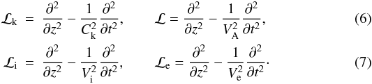 Ck
is the fast kink speed determined by
Ck
is the fast kink speed determined by 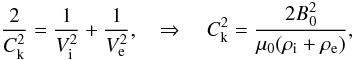 (8)where
B0 is the (constant) magnitude of the equilibrium magnetic
field, and μ0 the magnetic permeability of free space. In our
analysis, we use the equation for kink oscillations in a straight magnetic tube, derived in
Paper I, using the thin tube approximation. The thin tube approximation means that the
z component of the induction equation reduces to (3) to leading order in a series expansion in
powers of the radial coordinate. The plasma is only incompressible to leading order. Paper I
considers a cold plasma in the presence of background flow but here we consider the static
background case.
(8)where
B0 is the (constant) magnitude of the equilibrium magnetic
field, and μ0 the magnetic permeability of free space. In our
analysis, we use the equation for kink oscillations in a straight magnetic tube, derived in
Paper I, using the thin tube approximation. The thin tube approximation means that the
z component of the induction equation reduces to (3) to leading order in a series expansion in
powers of the radial coordinate. The plasma is only incompressible to leading order. Paper I
considers a cold plasma in the presence of background flow but here we consider the static
background case.
Equations (3)–(5) are solved inside the tube
(r < R − l/2
with ξr and
ξϕ only functions of z
and t) and in the external region
(r > R + l/2
with ξr and
ξϕ proportional to
1/r2 in the thin tube limit). The external
solutions are expressed in terms of the internal solutions by integrating the solutions to
the equations across the transition layer
(R − l/2 < r < R + l/2).
We define the internal solutions, using the thin tube approximation, as 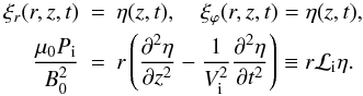 (9)Following
Paper I and the brief derivation in the Appendix (see Sect. A.2 and Eq. (A.6)), we obtain the
equation governing the propagation of the radial component of the fast kink mode,
η(z,t), namely
(9)Following
Paper I and the brief derivation in the Appendix (see Sect. A.2 and Eq. (A.6)), we obtain the
equation governing the propagation of the radial component of the fast kink mode,
η(z,t), namely 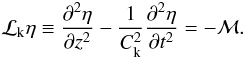 (10)The right-hand side of
Eq. (10) describes the damping of the fast
kink mode. When the right-hand side is zero, the kink wave propagates undamped from the
photospheric boundary. When ℳ is non-zero inside the transition layer, the energy in the
kink wave (as identified by η) is converted into the resonant Alfvén mode
(as identified by the spatial growth in amplitude of
ξϕ at the location where the value of the
variable Alfvén speed equals the kink speed Ck, i.e. where
VA(rs) = Ck).
(10)The right-hand side of
Eq. (10) describes the damping of the fast
kink mode. When the right-hand side is zero, the kink wave propagates undamped from the
photospheric boundary. When ℳ is non-zero inside the transition layer, the energy in the
kink wave (as identified by η) is converted into the resonant Alfvén mode
(as identified by the spatial growth in amplitude of
ξϕ at the location where the value of the
variable Alfvén speed equals the kink speed Ck, i.e. where
VA(rs) = Ck).
The quantity ℳ on the right-hand side of Eq. (10) is given by (see Appendix, Eq. (A.6)) 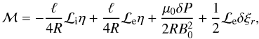 (11)where
δP = Pe − Pi and
δξr = ξe − η
are the jumps of P and ξr
across the transition layer.
(11)where
δP = Pe − Pi and
δξr = ξe − η
are the jumps of P and ξr
across the transition layer.
In what follows, we use the thin tube thin boundary (TTTB) approximation, and so have
ϵ = l/R ≪ 1. Hence,
the leading order approximation to ℳ, with respect to ϵ, is given in the
Appendix (see Eq. (A.11)) and the
propagating kink mode equation can be expressed as  (12)
(12)
3. Derivation of the governing equation
To progress, the integral involving ξϕ in
Eq. (12) must be expressed in terms of
η. Hence, we need to obtain the solution
for ξϕ in the transition layer. Thus, we
must solve Eq. (5), where the right hand side
is replaced by the leading order solution, i.e. with P replaced by
Pi and r by R. Next we use
Eq. (A.2), from the Appendix, to give to
leading order  (13)Below, we assume that the
photospheric driver at z = 0 excites a linearly polarized kink wave with
frequency ω propagating in the positive z-direction. In
the absence of the inhomogeneous annulus, the solution to Eq. (12) describes a constant amplitude, propagating wave for the internal
displacement that propagates with the speed Ck. The
perturbations of all variables, in this case, are functions of
T = t − z/Ck
only and, for a fixed frequency ω, have the form
eiωT. Due to the transition layer, the amplitude of the
internal displacement, η, is resonantly damped and for
ϵ ≪ 1 the lengthscale for the damping will be much longer than the
wavelength
L = 2πCk/ω
of the undamped kink wave. We do not prescribe the relationship between the wavelength and
the characteristic scale of the amplitude variation, but only assume that this scale is much
larger than L. Inside the transition layer we define a stretched radial
coordinate, namely
(13)Below, we assume that the
photospheric driver at z = 0 excites a linearly polarized kink wave with
frequency ω propagating in the positive z-direction. In
the absence of the inhomogeneous annulus, the solution to Eq. (12) describes a constant amplitude, propagating wave for the internal
displacement that propagates with the speed Ck. The
perturbations of all variables, in this case, are functions of
T = t − z/Ck
only and, for a fixed frequency ω, have the form
eiωT. Due to the transition layer, the amplitude of the
internal displacement, η, is resonantly damped and for
ϵ ≪ 1 the lengthscale for the damping will be much longer than the
wavelength
L = 2πCk/ω
of the undamped kink wave. We do not prescribe the relationship between the wavelength and
the characteristic scale of the amplitude variation, but only assume that this scale is much
larger than L. Inside the transition layer we define a stretched radial
coordinate, namely  (14)The definitions of
important variables used in this paper are given in Table 1.
(14)The definitions of
important variables used in this paper are given in Table 1.
Thus, we look for solutions for η of the form  (15)where
k = ω/Ck,
and assume
(15)where
k = ω/Ck,
and assume  (16)To keep the expressions
as simple as possible, we restrict our attention to the linear density profile. Thus, inside
the transition layer,
(16)To keep the expressions
as simple as possible, we restrict our attention to the linear density profile. Thus, inside
the transition layer, ![Mathematical equation: \begin{displaymath} \rho = \frac{1}{2}\left [ \rho_{\rm i} + \rho_{\rm e} - (\rho_{\rm i} - \rho_{\rm e})X\right ]. \end{displaymath}](/articles/aa/full_html/2013/03/aa20617-12/aa20617-12-eq67.png) In addition, we must
specify boundary conditions for η and
ξϕ on the driven boundary at
z = 0. We assume
In addition, we must
specify boundary conditions for η and
ξϕ on the driven boundary at
z = 0. We assume  and
and 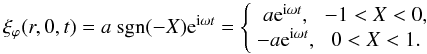 (17)From
the integral of Eq. (3), so that
(17)From
the integral of Eq. (3), so that
 and continuity of
ξr, the leading order boundary condition for
ξr on z = 0 is
ξr(r,z = 0,t) = aeiωt.
This choice matches the form of the undamped kink mode. We remind the reader that terms
proportional to ϵ are dropped to leading order.
and continuity of
ξr, the leading order boundary condition for
ξr on z = 0 is
ξr(r,z = 0,t) = aeiωt.
This choice matches the form of the undamped kink mode. We remind the reader that terms
proportional to ϵ are dropped to leading order.
Definitions of variables and parameters used in this paper.
The solution to (13) is obtained by the
method of Variations of Parameters (Boyce & DiPrima 2008). Thus, we set  (18)where
α(r,z) and β(r,z) are
to be determined. We define the ratio of the kink speed to the Alfvén speed as
χ = Ck/VA.
(18)where
α(r,z) and β(r,z) are
to be determined. We define the ratio of the kink speed to the Alfvén speed as
χ = Ck/VA.
Hence,  where
κ = (ρi − ρe)/(ρi + ρe).
Substituting these results into Eq. (13), we
have the pair of equations
where
κ = (ρi − ρe)/(ρi + ρe).
Substituting these results into Eq. (13), we
have the pair of equations 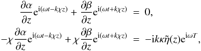 (19)and
the solutions to these equations are
(19)and
the solutions to these equations are 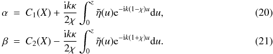 When
deriving the second equation in Eq. (19), we
neglect the small terms containing the derivatives of
When
deriving the second equation in Eq. (19), we
neglect the small terms containing the derivatives of
 in the right-hand side. Since the
wavelength associated with
e − ik(1 + χ)z is much
less that the damping length of η, we can integrate by parts (or
equivalently average over one wavelength) the expression for β and get,
approximately,
in the right-hand side. Since the
wavelength associated with
e − ik(1 + χ)z is much
less that the damping length of η, we can integrate by parts (or
equivalently average over one wavelength) the expression for β and get,
approximately,  (22)To eliminate any downward
propagating waves, we choose
(22)To eliminate any downward
propagating waves, we choose  (23)so that
 (24)Hence, there is no
contribution from downward propagating waves, as expected, and only the term due to the
upward propagating kink wave remains.
(24)Hence, there is no
contribution from downward propagating waves, as expected, and only the term due to the
upward propagating kink wave remains.
Integration by parts cannot be used for simplifying α
near X = 0, since the wavelength of the integrand,
2π/k(1 − χ), is no
longer less than the damping length. However, we can use that approach at
X = −1 (or equivalently at
r = R − l/2) to
confirm that  there.
Finally, we need to choose C1(X) so that the
boundary condition at z = 0, Eq. (17), is satisfied. Hence,  (25)This is the only
place where the spatial form of the photospheric driver appears, namely the first term on
the right hand side of Eq. (25). Thus, the
solution for ξϕ is
(25)This is the only
place where the spatial form of the photospheric driver appears, namely the first term on
the right hand side of Eq. (25). Thus, the
solution for ξϕ is 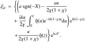 (26)There
are four terms in the expression for ξϕ, with
the first term dependent on the radial form of the boundary condition at
z = 0. The exponential factor for the undamped kink mode,
eiωT, has been taken outside the curly brackets, leaving a
complex function of kz, X and
(26)There
are four terms in the expression for ξϕ, with
the first term dependent on the radial form of the boundary condition at
z = 0. The exponential factor for the undamped kink mode,
eiωT, has been taken outside the curly brackets, leaving a
complex function of kz, X and
 inside.
Next, we must integrate Eq. (26) across the
transition layer. This is done term by term in the Appendix. The final equation governing
the propagation and damping of the kink mode, on using Eq. (15) for the form of η, is ![Mathematical equation: \begin{eqnarray} \label{eq:propkink} - 2 {\rm i} \frac{{\rm d}\tilde{\eta}}{{\rm d}s} &+& \frac{{\rm d}^2\tilde{\eta}}{{\rm d}s^2} = \frac{\epsilon \kappa}{4}\int_{-1}^{1} \xi_\varphi {\rm d}X = \frac{\epsilon \kappa}{4}\Bigg \{ F(s) \nonumber \\ && +\int_{0}^{s}\tilde{\eta} (u)g(s-u){\rm d}u + \tilde{\eta}(s)\ln \left [\frac{p_4}{p_3}\right ] \Bigg \} \end{eqnarray}](/articles/aa/full_html/2013/03/aa20617-12/aa20617-12-eq112.png) (27)on
cancelling the common factor of eiωT and setting
s = kz. In deriving Eq. (27), we have only applied the operator ℒe to the multiplier
eiωT. The additional terms are small for s
greater than unity. They are also small for κ ≪ 1. The inhomogeneous term
is given by
(27)on
cancelling the common factor of eiωT and setting
s = kz. In deriving Eq. (27), we have only applied the operator ℒe to the multiplier
eiωT. The additional terms are small for s
greater than unity. They are also small for κ ≪ 1. The inhomogeneous term
is given by ![Mathematical equation: \begin{eqnarray} \label{eq:inhomogen} F(s)&=& - \frac{4 a}{\kappa s^2} - {\rm i} \frac{4 a}{\kappa s} + \frac{2 a}{\kappa s^2}\left ({\rm e}^{{\rm i} s p_1}+ {\rm e}^{{\rm i} s p_2}\right )\nonumber \\ &&+\ {\rm i} \frac{2 a}{\kappa s} \left (\sqrt{1-\kappa}{\rm e}^{{\rm i} s p_1} + \sqrt{1+\kappa}{\rm e}^{{\rm i} s p_2}\right )\nonumber \\ &&+a {\rm e}^{{\rm i} 2s} \left [ \hbox{Ci}( s p_3)- \hbox{Ci}(s p_4)- {\rm i} \hbox{Si}(s p_3) + {\rm i} \hbox{Si}(s p_4)\right ], \end{eqnarray}](/articles/aa/full_html/2013/03/aa20617-12/aa20617-12-eq116.png) (28)and
(28)and
 (29)We define, for
later use, the complex function
(29)We define, for
later use, the complex function  (30)In Eqs. (27)–(29), we have used the shorthand notation,
  (31)and
Ci(x) and Si(x) are the cosine integral
and the sine integral, as defined in Abramowitz & Stegun
(1965) and the Appendix.
(31)and
Ci(x) and Si(x) are the cosine integral
and the sine integral, as defined in Abramowitz & Stegun
(1965) and the Appendix.
When κ is not too large, i.e. less than about 1/2, we
can use the approximations
p1 ≈ κ/2 and
p2 ≈ −κ/2 and express
F(s) as 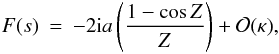 (32)where
Z = κkz/2. This approximation is
valid for κ ≪ Z ≪ 1/κ.
A more accurate representation of F, by taking an extra term in the
κ expansions of p1 and
p2 is given by
(32)where
Z = κkz/2. This approximation is
valid for κ ≪ Z ≪ 1/κ.
A more accurate representation of F, by taking an extra term in the
κ expansions of p1 and
p2 is given by 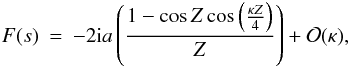 (33)by
considering variations over the slower spatial scale given by
κZ/4 = κ2kz/8.
Note that the Taylor series expansion for small κZ/4
gives the same approximation as Eq. (32).
The difference between the two approximations only occurs for large
κZ/4 and remains bounded. In addition, the expansion
for small Z agrees with small kz expansion discussed
below. Hence, the approximation given by Eq. (32) remains accurate for
0 < Z < 4/κ.
(33)by
considering variations over the slower spatial scale given by
κZ/4 = κ2kz/8.
Note that the Taylor series expansion for small κZ/4
gives the same approximation as Eq. (32).
The difference between the two approximations only occurs for large
κZ/4 and remains bounded. In addition, the expansion
for small Z agrees with small kz expansion discussed
below. Hence, the approximation given by Eq. (32) remains accurate for
0 < Z < 4/κ.
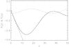 |
Fig. 1 Imaginary part of F(s) shown as a solid curve and small z expansion shown as a dot-dashed curve, for κ = 1/3. The real part of F(s) is the dotted curve. The approximation to the imaginary part of F(s) given by (33) is the dashed curve. |
4. Investigation of damping
In this section we investigate the spatial form of the damping of the kink mode. Firstly, we show that for small distances the amplitude decays Gaussianally and that this behaviour is not due to the specific form of the photospheric driver. Next we investigate a simple expansion in powers of ϵ, the ratio of the width of the transition layer to the radius of the flux tube. This illustrates that the simple expansion breaks down once a certain distance is reached. Finally, we use an expansion valid for small density ratios to derive a relatively simple looking equation to describe the damping. This form of equation allows us to investigate commonly used assumptions in the next subsection and demonstrates the importance of the various terms involved.
4.1. Small kz
Let us use Eq. (27) to study the
properties of propagating kink waves. We start our analysis by investigating the solution
of this equation for small kz. In the Appendix, we show that the
expansion of F(s) on the right-hand side of Eq. (27) is given by, (see Sects. A.4.1 and A.4.2),
![Mathematical equation: \begin{eqnarray} F(s) &\approx& {\rm i} s {\cal B} - a\left (1 + 2 {\rm i} s\right ) \ln \left [ \frac{1 + \sqrt{1 + \kappa}}{1 + \sqrt{1 - \kappa}} \right ] \nonumber \\ & &+ {\rm i} s a \left (\sqrt{1 + \kappa} - \sqrt{1 - \kappa} \right ), \end{eqnarray}](/articles/aa/full_html/2013/03/aa20617-12/aa20617-12-eq137.png) (34)where
(34)where
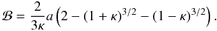 (35)For example, for
κ = 1/3, the linear approximation provides a good
fit to both F(s) and the coefficient of
out to s ≈ 5 (see Fig. 1). In this
case, small s means 0 ≤ s < 5.
Therefore, we can express Eq. (27) as
(35)For example, for
κ = 1/3, the linear approximation provides a good
fit to both F(s) and the coefficient of
out to s ≈ 5 (see Fig. 1). In this
case, small s means 0 ≤ s < 5.
Therefore, we can express Eq. (27) as
![Mathematical equation: \begin{eqnarray} - 2 {\rm i} \frac{{\rm d}\tilde{\eta}}{{\rm d}s} + \frac{{\rm d}^2\tilde{\eta}}{{\rm d}s^2} &=& \frac{\epsilon \kappa}{4}\left \{ {\rm i} s {\cal B} - 2 {\rm i} s a \ln \left [\frac{1 + \sqrt{1 + \kappa}}{1 + \sqrt{1 - \kappa}}\right ]\right . \nonumber \\ & &\left . + 2 {\rm i} s a \left [\sqrt{1 + \kappa} - \sqrt{1 - \kappa} \right ]\right . \nonumber \\ & & \left . + {\rm i} \int_{0}^{s}\left (\tilde{\eta}(u) - a\right ) \left [\sqrt{1 + \kappa} - \sqrt{1 - \kappa}\right ]{\rm d}u \right .\nonumber \\ & &\left .+\left (\tilde{\eta}(s) - a\right ) \ln \left [ \frac{1 + \sqrt{1 + \kappa}}{1 + \sqrt{1 - \kappa}} \right ]\right \}\cdot \label{eq:smallz} \end{eqnarray}](/articles/aa/full_html/2013/03/aa20617-12/aa20617-12-eq141.png) (36)When
κ is not too close to unity,
κ < 1, Eq. (36) can be approximated by
(36)When
κ is not too close to unity,
κ < 1, Eq. (36) can be approximated by 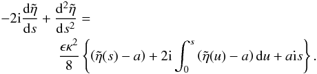 (37)This
form of the equation is used to illustrate the method of analysis with the result for more
general κ listed below. Since
(37)This
form of the equation is used to illustrate the method of analysis with the result for more
general κ listed below. Since  when ϵ = 0, we
set
when ϵ = 0, we
set  and, in the weak damping
limit and for small values of s, terms containing
and, in the weak damping
limit and for small values of s, terms containing
 on the right hand side of
Eq. (36) can be neglected. Hence, the
on the right hand side of
Eq. (36) can be neglected. Hence, the
 equation is
 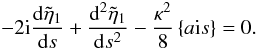 (38)The solution is to
this equation is the complementary function and a particular integral. Since it has to
satisfy the boundary condition , it contains only one
arbitrary constant. To determine this constant, we once again use the condition that there
is no downward propagating wave. As a result we obtain
(38)The solution is to
this equation is the complementary function and a particular integral. Since it has to
satisfy the boundary condition , it contains only one
arbitrary constant. To determine this constant, we once again use the condition that there
is no downward propagating wave. As a result we obtain 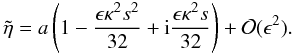 (39)It is common in
considering the effect of weak damping, where
(39)It is common in
considering the effect of weak damping, where  , to assume that the second
derivative will be
, to assume that the second
derivative will be  ,
i.e. smaller than the first derivative. However, this is not the case, as shown by
Eq. (39). Instead the imaginary term in
Eq. (39) results from keeping the second
derivative. The amplitude of
is, however,
,
i.e. smaller than the first derivative. However, this is not the case, as shown by
Eq. (39). Instead the imaginary term in
Eq. (39) results from keeping the second
derivative. The amplitude of
is, however,  and this can be obtained
directly from Eq. (37) by dropping the
second derivative. Thus, the second derivative term modifies the phase of the weakly
damped kink mode.
and this can be obtained
directly from Eq. (37) by dropping the
second derivative. Thus, the second derivative term modifies the phase of the weakly
damped kink mode.
Repeating the above method for general κ, we can show that, for small
s, ![Mathematical equation: \begin{equation} \tilde{\eta} \approx a[1 - \epsilon q(\kappa)(s)^2] \label{eq:4.1} \end{equation}](/articles/aa/full_html/2013/03/aa20617-12/aa20617-12-eq154.png) (40)where
(40)where
![Mathematical equation: \begin{eqnarray} \label{eq:4.2} q(\kappa) &=& \frac1{24}\left[2 - (1 - 2\kappa)\sqrt{1 + \kappa} - (1 + 2\kappa)\sqrt{1 - \kappa}\right]\nonumber \\ & & + \frac\kappa8\ln\frac{1 + \sqrt{1 - \kappa}}{1 + \sqrt{1 + \kappa}} \cdot \end{eqnarray}](/articles/aa/full_html/2013/03/aa20617-12/aa20617-12-eq155.png) (41)It
is worth noting that
(41)It
is worth noting that  (42)with
the accuracy better than 2.5% for
0 < κ < 1. This
approximation for q can be used even for values of κ
close to unity. For example, when the density contrast is 10 so that
κ = 9/11, the maximum error in replacing Eq. (41) by the simpler expression of Eq. (42) is less than 1.6%.
(42)with
the accuracy better than 2.5% for
0 < κ < 1. This
approximation for q can be used even for values of κ
close to unity. For example, when the density contrast is 10 so that
κ = 9/11, the maximum error in replacing Eq. (41) by the simpler expression of Eq. (42) is less than 1.6%.
To clearly highlight the behaviour of the damping, we investigate the logarithm of
so that, for example,
e−z/L would appear as
a straight line. For our expansion given by Eq. (40), we have 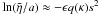 , where
s = kz. This is consistent with
, where
s = kz. This is consistent with
 but there are other
functions which have the same initial terms in their expansion. For example,
but there are other
functions which have the same initial terms in their expansion. For example, 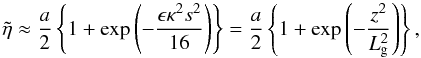 (43)where
 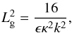 (44)is a slightly better fit
to the numerical solution provided s is not too
large. Here not too large means up to a distance of approximately a wavelength
divided by κ from the boundary driver. Since the long wavelength limit is
used, this can be a significant distance from the location of the driver.
(44)is a slightly better fit
to the numerical solution provided s is not too
large. Here not too large means up to a distance of approximately a wavelength
divided by κ from the boundary driver. Since the long wavelength limit is
used, this can be a significant distance from the location of the driver.
Thus, the amplitude of
decreases Gaussianally for small s. Although the series given by
Eq. (40) is the correct expression for
small s, this can be expressed by a number of different functional forms
that have the same expansion for small s.
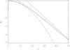 |
Fig. 2
|

4.2. Expansion in powers of ϵ
Before progressing, we study the approximations to
F(s) = Fr(s) + iFi(s).
Figure 1 shows that the imaginary part of
F(s),
Fi(s), dominates
Fr(s), for
0 < s < 30, and the
small s expansion is valid out to s = 5. Note that
Eq. (33) provides a good fit to
Fi(s) for
0 < s < 50, as seen in
Fig. 1. Now we look to express
in powers of ϵ as  . Hence,
 . Since both the imaginary parts
of F(s) and G(s) are
larger than the respective real parts, we drop the real parts. Dropping the second
derivative, we have
. Since both the imaginary parts
of F(s) and G(s) are
larger than the respective real parts, we drop the real parts. Dropping the second
derivative, we have  (45)Hence,
 (46)This is shown is
Fig. 2. Our simple expansion in powers of
ϵ must break down whenever
(46)This is shown is
Fig. 2. Our simple expansion in powers of
ϵ must break down whenever  becomes of order unity. This secular behaviour suggests that there is a slower lengthscale
associated with the damping of the kink mode. However, this slow scale is not simply a
linear combination of ϵ and z.
becomes of order unity. This secular behaviour suggests that there is a slower lengthscale
associated with the damping of the kink mode. However, this slow scale is not simply a
linear combination of ϵ and z.
Thus, the expansion in powers of ϵ is only valid for small enough
distances, such that  . For large distances, this
expansion will always break down. However, the distance where it begins to break down does
depend strongly on ϵ. For small enough ϵ, we can clearly
see how the form of the damping is initially Gaussian in character but it switches to an
almost linear form further up. If ϵ is larger, but still less than unity,
the expansion will be valid for the Gaussian part only.
. For large distances, this
expansion will always break down. However, the distance where it begins to break down does
depend strongly on ϵ. For small enough ϵ, we can clearly
see how the form of the damping is initially Gaussian in character but it switches to an
almost linear form further up. If ϵ is larger, but still less than unity,
the expansion will be valid for the Gaussian part only.
4.3. Expansion in powers of κ
Returning to the kink mode Eq. (27), we
expand the right hand side in powers of κ. Defining the new independent
variable Z = κkz/2, the equation is
 Hence,
the second order derivative can be neglected to leading order in κ and
the weak density variation assumption κ ≪ 1 leads to
Hence,
the second order derivative can be neglected to leading order in κ and
the weak density variation assumption κ ≪ 1 leads to  (47)Equation (47) is the important equation that can be used
to investigate the spatial damping of the propagating kink mode, whenever the density
contrast is not too large. For example, good agreement is found with the numerical
solutions (see Sect. 5) whenever
ρi/ρe ≤ 3 or
equivalently κ ≤ 1/2. The advantage of Eq. (47) over the full expression in Eq. (27) is its relative simplicity. This equation
can be solved numerically. We can use it also to investigate how some standard
approximations compare with the full solution. In addition, the inhomogeneous term in
Eq. (47) is derived directly from the
imposed form of the photospheric driver. Changing the driver changes this one term.
However, as we will see below, neglecting this term does not change the conclusion that
the damping is Gaussian in nature over the first few wavelengths. It is just that the rate
of the Gaussian damping is different.
(47)Equation (47) is the important equation that can be used
to investigate the spatial damping of the propagating kink mode, whenever the density
contrast is not too large. For example, good agreement is found with the numerical
solutions (see Sect. 5) whenever
ρi/ρe ≤ 3 or
equivalently κ ≤ 1/2. The advantage of Eq. (47) over the full expression in Eq. (27) is its relative simplicity. This equation
can be solved numerically. We can use it also to investigate how some standard
approximations compare with the full solution. In addition, the inhomogeneous term in
Eq. (47) is derived directly from the
imposed form of the photospheric driver. Changing the driver changes this one term.
However, as we will see below, neglecting this term does not change the conclusion that
the damping is Gaussian in nature over the first few wavelengths. It is just that the rate
of the Gaussian damping is different.
4.3.1. Expansion in powers of ϵ
Next, we can expand
in powers of ϵ and obtain  Evaluating the
integrals, we have
Evaluating the
integrals, we have  (48)where
γ ≈ 0.5772 is Euler’s constant and Ci(Z) and
Si(Z) are the Cosine and Sine integrals respectively (Abramowitz
& Stegun 1965). We can approximate
by
(48)where
γ ≈ 0.5772 is Euler’s constant and Ci(Z) and
Si(Z) are the Cosine and Sine integrals respectively (Abramowitz
& Stegun 1965). We can approximate
by 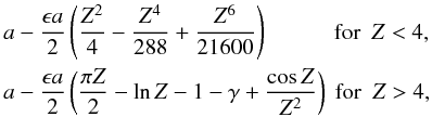 (49)where
the appropriate asymptotic expansions for Ci(Z) and
Si(Z) have been used. Note that the logarithm of
,
when ϵ is small, is simply
(49)where
the appropriate asymptotic expansions for Ci(Z) and
Si(Z) have been used. Note that the logarithm of
,
when ϵ is small, is simply  (50)This form is used when
comparing with the numerical solution for small ϵ in Sect. 5 below. From Eq. (49), we expect
(50)This form is used when
comparing with the numerical solution for small ϵ in Sect. 5 below. From Eq. (49), we expect  to
behave like
−ϵπZ/4 + (ϵlnZ)/2
for large Z, so that the Terradas et al. (2010) results will slightly over-estimate the damping rate due to the
neglect of the logarithmic term. The behaviour for small Z is again the
same as the real part of Eq. (39).
to
behave like
−ϵπZ/4 + (ϵlnZ)/2
for large Z, so that the Terradas et al. (2010) results will slightly over-estimate the damping rate due to the
neglect of the logarithmic term. The behaviour for small Z is again the
same as the real part of Eq. (39).
We remind the reader that, for large Z, the expansion in powers of
ϵ will break down whenever the magnitude of
becomes of order unity. The
small Z expansion, however, will remain valid for small
ϵ and κ.
4.4. Approximate solutions to Eq. (47)
Equation (47) can be solved numerically and the results are compared with the full numerical solution to the linear MHD equations (as discussed in Pascoe et al. 2012). This comparison is discussed in Sect. 5. Before that, we can use Eq. (47) to investigate commonly used approximations in the large z limit and compare these approximations with the numerical solution of Eq. (47).
4.4.1. Approximation 1
Firstly, consider the behaviour of  for
1 ≪ kz ≪ ϵ-1. The first term on the
right-hand side of Eq. (47) is
for
1 ≪ kz ≪ ϵ-1. The first term on the
right-hand side of Eq. (47) is
 when compared to the second term. Hence, we neglect the first term. Thus, for large
Z, we solve
when compared to the second term. Hence, we neglect the first term. Thus, for large
Z, we solve 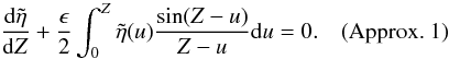 (51)where
Z = κkz/2. This approximate
equation can be solved by a Laplace transform but it is not straightforward to invert
the transform back to physical space. Instead we solve this equation numerically to
determine Approximation 1,
(51)where
Z = κkz/2. This approximate
equation can be solved by a Laplace transform but it is not straightforward to invert
the transform back to physical space. Instead we solve this equation numerically to
determine Approximation 1,  . Approximation 1 is shown
in Fig. 3 as a dashed curve.
. Approximation 1 is shown
in Fig. 3 as a dashed curve.
4.4.2. Approximation 2
Using the mean value theorem, the integral in Eq. (51) can be expressed as 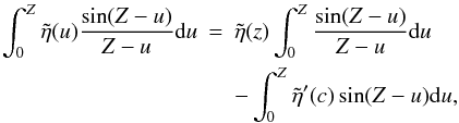 where
the derivative of
is evaluated at c and
u ≤ c ≤ Z. Since the derivative of
is ,
we neglect the second term. Hence, Eq. (51) reduces to
where
the derivative of
is evaluated at c and
u ≤ c ≤ Z. Since the derivative of
is ,
we neglect the second term. Hence, Eq. (51) reduces to 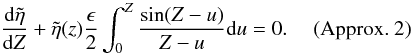 and
this can be solved by an integrating factor to give
and
this can be solved by an integrating factor to give 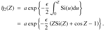 (52)For
large Z,
Si(Z) → π/2 and so
(52)For
large Z,
Si(Z) → π/2 and so 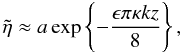 (53)as derived by Terradas
et al. (2010). This approximate solution is shown
in Fig. 3 as a dot-dashed curve. Despite neglecting
the inhomogeneous terms, which arise through the form of the photospheric driver when
solving for the resonant Alfvén mode inside the transition layer, this solution also has
a Gaussian form for small Z of the form
aexp { −ϵZ2/4 }
and only takes on the linear exponential damping for large Z. So the
inhomogeneous term only changes the value of the coefficient of
Z2 in the Gaussian damping.
(53)as derived by Terradas
et al. (2010). This approximate solution is shown
in Fig. 3 as a dot-dashed curve. Despite neglecting
the inhomogeneous terms, which arise through the form of the photospheric driver when
solving for the resonant Alfvén mode inside the transition layer, this solution also has
a Gaussian form for small Z of the form
aexp { −ϵZ2/4 }
and only takes on the linear exponential damping for large Z. So the
inhomogeneous term only changes the value of the coefficient of
Z2 in the Gaussian damping.
4.4.3. Approximation 3
Next we re-introduce the inhomogeneous term on the right-hand side of Eq. (47) but take the
outside the integral
again and investigate 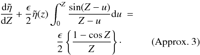 Again
we can use an integrating factor to obtain
Again
we can use an integrating factor to obtain ![Mathematical equation: \begin{eqnarray} \label{eq:solve} \tilde{\eta}_3(Z) &=& a \Bigg\{ \int_{0}^{Z} \frac{\epsilon}{2} \left [\frac{1 - \cos u}{u} \right ] \exp \left (\frac{\epsilon}{2}\int_{0}^{u} \hbox{Si}(s) {\rm d}s\right ){\rm d}u \nonumber \\ & & + 1\Bigg\}\exp \left (-\frac{\epsilon}{2}\int_{0}^{Z} \hbox{Si}(u) {\rm d}u\right ). \end{eqnarray}](/articles/aa/full_html/2013/03/aa20617-12/aa20617-12-eq213.png) (54)The
first term in curly brackets on the right-hand side is due to the inhomogeneous term,
while the second term is the same as Approximation 2.
(54)The
first term in curly brackets on the right-hand side is due to the inhomogeneous term,
while the second term is the same as Approximation 2.
 is shown as the triple
dot-dashed curve in Fig. 3. Note that for small
Z this approximation has the form
is shown as the triple
dot-dashed curve in Fig. 3. Note that for small
Z this approximation has the form 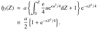 (55)As
shown above in Eq. (43), this
approximate solution has the same Taylor series expansion as the small
z expansion derived earlier.
(55)As
shown above in Eq. (43), this
approximate solution has the same Taylor series expansion as the small
z expansion derived earlier.
Finally, we can solve Eq. (51)
numerically to determine the validity of using the mean value theorem to derive
Approximation 3. The numerical result for
is shown in Fig. 3 as the solid curve.
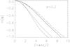 |
Fig. 3 Different approximations for |
There is a significant difference between the approximate solutions
 ,
,
 and
when Z
is sufficiently large. The neglect of the inhomogeneous term, Approximations 1 and 2,
changes the coefficient of the Gaussian term at small Z and results in
too much damping. However, it still remains Gaussian in nature. For larger
Z, Approximation 1 is more or less parallel to the numerical solution
to Eq. (47). Approximation 2 damps
significantly faster. Approximation 3 includes the inhomogeneous term but the
simplifying assumption of taking
outside the integral predicts a slower damping rate at large Z.
However, it does have the correct behaviour for small Z.
and
when Z
is sufficiently large. The neglect of the inhomogeneous term, Approximations 1 and 2,
changes the coefficient of the Gaussian term at small Z and results in
too much damping. However, it still remains Gaussian in nature. For larger
Z, Approximation 1 is more or less parallel to the numerical solution
to Eq. (47). Approximation 2 damps
significantly faster. Approximation 3 includes the inhomogeneous term but the
simplifying assumption of taking
outside the integral predicts a slower damping rate at large Z.
However, it does have the correct behaviour for small Z.
The best approach in understanding the spatial damping of the kink mode through mode coupling to the Alfvén mode in the transition layer, is to solve Eq. (47) numerically. Keeping in mind the results shown in Fig. 3, the error in using Approximation 3 is not too significant. It has the advantage of having a solution in a closed analytical form. The functions Si and Ci are rapidly obtained from computer algebra packages, such as Maple, and it is easy to use a package to numerically integrate the terms in Eq. (54). The small Z expansion, using Eq. (54) gives the correct Gaussian behaviour.
5. Comparison with numerical results
The numerical solution to the linear MHD equations remains the most accurate description of the damped kink mode. In this section, the approximate solutions derived (and the methods illustrated) in the previous section are compared with the actual numerical results. Two different numerical codes are used, a second order Lax-Wendroff scheme and a fourth order, finite difference method. The numerical results obtained with the two different methods are consistent and indicate that the results obtained are not dependent on the method used to solve the linear MHD equations. We consider two examples for a small transition layer, namely small ϵ (ϵ < κ < 1) and a small density contrast (κ < ϵ < 1).
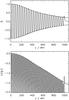 |
Fig. 4 Amplitude of η = ξr and logarithm of the modulus of η at the centre of the tube shown as functions of distance z. The solid curve represents the numerical solution, the dashed curve is the numerical solution of (47). The period is 36 s, the ratio of the width of the transition layer to the radius is 0.2 and the density ratio, ρi/ρe = 1.3. |
Figure 4 shows the results for a period of 36 s, a width of the transition layer to radius ratio of 0.2 and a density contrast of 1.3. Thus, we have ϵ = 0.2 and κ ≈ 0.13 and the small κ Eq. (47) is appropriate. The solution to Eq. (47), namely the amplitude of the kink mode, is shown as a dashed curve, while the solid curve is the full numerical solution for the kink mode, ξr, on the axis, r = 0. The agreement is extremely good for all distances apart from the leading initial wavelength. To illustrate the actual form of the damping the logarithm of the absolute value of ξr is also shown. What is clear is how the behaviour of the damping is Gaussian for small distances, as shown in Sect. 4, and switches to almost linear for larger distances. Despite having ϵ = 0.2, the TTTB equation provides an extremely good fit to the full solution. This is because the density ratio is only 1.3 and the important parameter κ is small. Thus, the damping is weak and Eq. (47) provides a good approximation.
Next we consider the situation where the period is 24 s, which is just long enough for the long wavelength limit to apply, the width of the transition layer to radius ratio is small (ϵ = 0.05) and the density contrast is 2 (κ = 1/3). Note that the value of κ is still quite small and we expect Eqs. (48) and (49) to give a good approximation. The comparison is shown in Fig. 5.
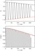 |
Fig. 5 Amplitude of η = ξr and logarithm of the modulus of η at the centre of the tube shown as functions of distance z. The solid curve represents the numerical solution using the fourth order scheme, the dashed curve is the numerical solution of Eq. (47) and the red solid curve is the small ϵ solution given by Eq. (48). The period is 24 s, the width of the transition layer is 0.05 and the density ratio, ρi/ρe = 2. |
As above, the dashed curve in Fig. 5 outlines the amplitude of the kink mode, by solving Eq. (47). In addition, the solid curve is the result of the small ϵ expansion given by Eq. (48). Both of the approximations match with the numerical solution to the linear MHD equations, showing that, although the small κ equation has a relatively simple form, the solution provides excellent agreement with the numerical solution.
Finally, we show the results for a density contrast of 10, period of 48 s and ϵ = 0.05 in Fig. 6. For these parameters, the thin tube, thin boundary analysis is still appropriate. However, what is not so clear is whether the small κ description is still relevant. From Sect. 4.1, we expect the form of the Gaussian profile to be unaffected by the large density contrast, since the approximation given by Eq. (42), is accurate to better than 2% for this choice. Hence, the initial Gaussian part still provides an excellent approximation. In addition, at large z, the damping will approach the limit predicted by Terradas et al. (2010) and, with the small and large z limits fixed, the approximation given by the solution to Eq. (47) continues to give an excellent fit to the numerical results.
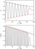 |
Fig. 6 Line styles as in Fig. 5. The period is 48 s, the width of the transition layer is 0.05 and the density ratio, ρi/ρe = 10. |
6. Conclusions
So which approximations should one use in analysing observations of propagating kink modes? For the magnetic flux tube considered in this paper, if the density contrast is large, then the full damped kink mode equation, Eq. (27), is used. However, if the density contrast is smaller than about 3, then solutions to the small κ equation, Eq. (47), agree with the full numerical results. The solution to Eq. (47) can be approximated by the analytical solution of Approximation 3, Eq. (54), where the Sine Integral, Si, is readily computed in various computer algebra packages.
The different approximations used in solving Eq. (47) show clearly that the Gaussian behaviour for small distances is not just due to the form of driving on the boundary. It appears in the homogeneous kink mode equation as well, when the radial profile of ξr on z = 0 is completely ignored. However, the form of the boundary driver does influence the value of the coefficient of the Gaussian term. It is possible to eliminate the Gaussian damping by selecting a very specific photospheric driving profile, that has strong localised variations inside the transition layer. Any smoother profile will result in the Gaussian behaviour noted in this paper.
The nature of the damping of the kink mode changes at larger distances to roughly linear, although there is really a series solution here which varies gently over several wavelengths. The change in character from Gaussian to “almost linear” occurs between the values of Z = 2 and Z = 4 and is essentially independent of the width of the transition layer. If L is the wavelength of the undamped kink mode, this change over distance can be expressed in terms of L as 2L/πκ and 4L/πκ. For a density ratio of 2, or κ = 1/3, the Gaussian behaviour is appropriate for at least 2 to 3 wavelengths, while a density ratio of 1.3 (κ = 0.13), on the other hand, it is valid for 5 to 10 wavelengths.
The small-κ equation is a relatively simple equation that can be used to investigate the damping of the kink mode and the coupling to the Alfvén mode in the transition layer. While both κ and ϵ should be small, whether κ < ϵ or visa-versa is unimportant. The comparison between the predictions of the small-κ equation and the full numerical solution is extremely good for the cases shown. However, a detailed parameter study is necessary to determine how good the small-κ assumption is (see Pascoe et al. 2013). This also determines how to use both the Gaussian and linear damping rates when analysing observations of propagating kink waves.
There are several possible extensions to this work, such as including stratification, field line curvature and magnetic field expansion. The density decrease in the direction of wave propagation is known to modify the amplitude of the velocity and magnetic field perturbations, increasing one and decreasing the other so that, when the wavelength is less than the stratification length, the perturbed Poynting flux remains constant. Most recently Soler et al. (2011b) have investigated the effect of stratification. When the density is decreasing away from the location of the driver, there is a competition between the increase in amplitude, due to the stratification, and a decrease due to the damping. Thus, we expect the same competition to occur between the Gaussian damping and the amplitude increase. If the density varies over a distance much shorter than the wavelength, there may be reflection.
The effect of field line curvature on the kink wave has been reviewed recently by Van Doorsselaere et al. (2009). For a semi-toroidal loop, the curved extension to the straight cylinder considered here, they find that curvature does not change either the normal mode frequency or the damping due to the narrow inhomogeneous layer. Only when ϵ, the ratio of the transition layer width to loop radius, is large is there a significant effect. However, large values of ϵ cannot be accurately treated by the Thin Tube, Thin Boundary approximation used here. The equations for the evolution of propagating, damped kink modes for large values of ϵ must be solved numerically (see Pascoe et al. 2013, in this issue).
The expansion of the flux tube cross section has been studied by, for example, De Moortel et al. (2000) and Smith et al. (2007). As the flux tube widens, the wavelength shortens. This will enhance the damping through mode coupling. However, the shortening of the wavelength will eventually invalidate the long wavelength assumption of the thin tube. If the expansion of the magnetic field is characterised by the length LA, we would expect the Gaussian damping to be the dominate effect for LA > Lg, where Lg is defined in Eq. (44). On the other hand, if LA < Lg, the Gaussian damping envelope is likely to be modified.
The Gaussian form of the damping demonstrated in this paper may be modified by the various extensions to the straight, unstratified plasma cylinder described above. However, it is clear that the straightforward application of a simple linear exponential damping, while easy to apply, may give misleading results. A detailed comparison of these results when used for coronal seismology, is discussed in the accompanying paper by Pascoe et al. (2013).
Throughout the paper we have used the term “mode coupling” to describe the conversion of energy from the compressional (kink-like) driven wave to an incompressible (Alfvén-like) wave. Both terms refer to the same physical processes, but in different situations, and “mode coupling/conversion” can be thought of as more general than the term “resonant absorption”. Consider the system of equations driven harmonically in time but studied with different boundary conditions. In this paper, the field lines are open and the axial wavenumber, k, is determined by the solution to these equations. If, on the other hand, the ends of the field lines are tied and it is the radial boundary that is driven, then the axial wavenumber becomes a discrete quantity. There is a large volume of papers considering this second case. The main features are that the global kink mode resonates at one particular radius, where its energy is absorbed, and its eigenfunction is singular here. The fact that the location of the singularity corresponds to a resonant matching of kink and natural Alfvén frequencies has led to this solution being termed “resonant” absorption. The solution we describe differs in that we do not have tied ends to our field lines, so there is no quantized k and no natural Alfvén frequency. Moreover, our solution does not have any singularities: there is simply an accumulation of energy around a particular radius, but there is no singularity. The location of energy accumulation may be identified by the matching the kink and Alfvén phase speeds (Allan & Wright 2000). Of course, if k was determined by line tied boundary conditions, then matching phase speeds is equivalent to matching natural frequencies. Finally, we note that there is no singularity in the solutions if the finite length loop case is studied as an initial value problem and is not driven continually in a harmonic manner.
This paper has presented a detailed mathematical derivation of the damping of propagating
kink waves. Amid all the mathematical expressions, there are only a few key results that are
necessary for applying these results in practice. A simple flow diagram, shown in Fig. 7, identifies the important equations to use and the
conditions under which they apply. Obviously the thin boundary assumption is essential in
deriving the appropriate expressions from integrating across the transition layer. Hence,
the results in this paper will provide useful results for ϵ ≲ 0.2. While
the general damped kink mode is described by Eq. (27), the much simpler equation, Eq. (47), that was derived only assuming κ ≪ 1, is applicable for all
density contrasts. Equation (47) can be
solved numerically but, if ϵ ≤ 0.05 then Eq. (48) provides a very good approximation to the damping envelope. Finally,
if 0.05 < ϵ ≲ 0.2, a useful approximation can be
derived on using  in Eq. (54) for general z
and Eq. (55) for small values
of κkz/2.
in Eq. (54) for general z
and Eq. (55) for small values
of κkz/2.
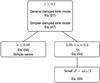 |
Fig. 7 Flow chart to identify the appropriate expressions to use. |
Online material
Appendix A: Derivation of kink mode equation
We give a short derivation of the basic equations, starting from Eqs. (3)–(5). The solutions are obtained in the three regions, inside the flux tube, outside the flux tube and in the transition layer.
A.1. Internal solution
Using the thin tube (or long wavelength) limit, the internal solutions can be
expressed as  (A.1)Hence, at
r = R − l/2 = R(1 − ϵ/2),
we have
(A.1)Hence, at
r = R − l/2 = R(1 − ϵ/2),
we have  (A.2)
(A.2)
A.2. External solution
Again using the thin tube limit, we have
 (A.3)Hence, at
r = R + l/2 = R(1 + ϵ/2),
we have
(A.3)Hence, at
r = R + l/2 = R(1 + ϵ/2),
we have  (A.4)Since both
ξr and P are
continuous across the transition layer as ϵ → 0, we can state
ξe = η + δξr, Pe = Pi + δP,
where both δξr and
δP tend to zero as ϵ → 0. Using (A.4), we have, correct to
O(ϵ2),
(A.4)Since both
ξr and P are
continuous across the transition layer as ϵ → 0, we can state
ξe = η + δξr, Pe = Pi + δP,
where both δξr and
δP tend to zero as ϵ → 0. Using (A.4), we have, correct to
O(ϵ2),  (A.5)Rearranging
Eq. (A.5), the final equation for
the propagating kink mode is
(A.5)Rearranging
Eq. (A.5), the final equation for
the propagating kink mode is  (A.6)Note that the
right hand side of (A.6) is of
O(ϵ). It is the leading order expressions for
δξr and
δP that we now need to calculate and this is done from the
transition layer solutions.
(A.6)Note that the
right hand side of (A.6) is of
O(ϵ). It is the leading order expressions for
δξr and
δP that we now need to calculate and this is done from the
transition layer solutions.
A.3. Transition layer solution
Integrating Eq. (3) across the thin
transition layer, we have ![Mathematical equation: \appendix \setcounter{section}{1} \begin{eqnarray} \left [ r \xi_r \right ]_{R-l/2}^{R+l/2} &=& R(1 + \epsilon/2)\xi_{\rm e} - R(1-\epsilon/2)\eta = \int_{R-l/2}^{R+l/2} \xi_\varphi {\rm d}r, \nonumber \\ \delta \xi_r + \epsilon \eta &=& \frac{1}{R}\int_{R-l/2}^{R+l/2} \xi_\varphi {\rm d}r + {\cal O}(\epsilon^2). \label{eq:A3} \end{eqnarray}](/articles/aa/full_html/2013/03/aa20617-12/aa20617-12-eq262.png) (A.7)Integrating
(4) we have
(A.7)Integrating
(4) we have
 (A.8)Remembering that
η is independent of r,
(A.8)Remembering that
η is independent of r,
 is l times
the average value of the operator ℒ and, for the linear density profile, the average
is ℒk, thus,
is l times
the average value of the operator ℒ and, for the linear density profile, the average
is ℒk, thus,  (A.9)since
ℒkη = O(ϵ). Hence, for
the linear density profile
(A.9)since
ℒkη = O(ϵ). Hence, for
the linear density profile  (A.10)
We substitute Eq. (A.7) into
Eq. (A.6) and, using both Eq. (A.10),
ℒi + ℒe = 2ℒk and that again
ℒkη = O(ϵ), this
results in the propagating kink mode equation  (A.11)
A.4. Integration of ξϕ across the transition layer
In this section we evaluate
 (A.12)Using the solution
for ξϕ given by (26), the integral across the transition
layer is made up of four terms. These are evaluated in turn.
(A.12)Using the solution
for ξϕ given by (26), the integral across the transition
layer is made up of four terms. These are evaluated in turn.
A.4.1. Term 1
Now the integral of the first term on the RHS of Eq. (26), due to the radial profile of the driving boundary condition
of ξϕ, is
![Mathematical equation: \appendix \setcounter{section}{1} \begin{displaymath} \begin{array}{l} \int_{-1}^{1} a\ \hbox{sgn}(-X) {\rm e}^{{\rm i}(\omega t - k \chi z)} {\rm d}X = a \int_{-1}^{0}{\rm e}^{{\rm i}(\omega t - k \sqrt{(1 - \kappa X)} z)} {\rm d}X - a \int_{0}^{1}{\rm e}^{{\rm i}(\omega t - k \sqrt{(1 - \kappa X)} z)} {\rm d}X\\[2mm] =- \left (\dfrac{4 a}{k^2 \kappa z^2} + {\rm i} \dfrac{4 a}{k \kappa z}\right ) {\rm e}^{{\rm i}\omega T} + \dfrac{2 a}{k^2 \kappa z^2}\left ({\rm e}^{{\rm i}(\omega t -k \sqrt{1 -\kappa}z)}+ {\rm e}^{{\rm i}(\omega t- k\sqrt{1 + \kappa}z)}\right )\\[4mm] + {\rm i} \dfrac{2 a}{k \kappa z}\left (\sqrt{1-\kappa}{\rm e}^{{\rm i}(\omega t - k\sqrt{1-\kappa}z)} + \sqrt{1+\kappa}{\rm e}^{{\rm i}(\omega t - k\sqrt{1+\kappa}z)}\right )\\[4mm] = - {\rm e}^{{\rm i}\omega T}\left [\dfrac{4 a}{k^2 \kappa z^2} + {\rm i} \dfrac{4 a}{k \kappa z} - \dfrac{2 a}{k^2 \kappa z^2}\left ({\rm e}^{{\rm i} k z( 1 - \sqrt{1 -\kappa})}+ {\rm e}^{{\rm i} k z( 1- \sqrt{1 + \kappa})}\right ) - {\rm i} \dfrac{2 a}{k \kappa z}\left (\sqrt{1-\kappa}{\rm e}^{{\rm i} k z(1 - \sqrt{1-\kappa})} + \sqrt{1+\kappa}{\rm e}^{{\rm i} k z( 1 - \sqrt{1+\kappa})}\right ) \right ] . \end{array} \end{displaymath}](/articles/aa/full_html/2013/03/aa20617-12/aa20617-12-eq275.png) For
large kz, this is proportional to
(kz)-1. The influence of the choice of boundary
condition does becomes less important after several wavelengths.
For
large kz, this is proportional to
(kz)-1. The influence of the choice of boundary
condition does becomes less important after several wavelengths.
For small values of kz, we can expand the result in a series to
show that the first term is  For small
κ, Term 1 can be expressed as
For small
κ, Term 1 can be expressed as
 where we have
defined
where we have
defined  (A.13)
A.4.2. Term 2
The second term on the RHS integrates to give ![Mathematical equation: \appendix \setcounter{section}{1} \begin{displaymath} \begin{array}{l} -\frac{a\kappa}{2}\int_{-1}^{1} \dfrac{{\rm e}^{{\rm i}(\omega t - k\sqrt{1 - \kappa X}z)}}{\chi (1 + \chi)} {\rm d}X = -\dfrac{a\kappa}{2} {\rm e}^{{\rm i}\omega T + {\rm i} 2kz} \int_{-1}^{1} \dfrac{{\rm e}^{- {\rm i} k z( 1 + \sqrt{1 - \kappa X})}}{\sqrt{1-\kappa X}(1 + \sqrt{1 - \kappa X})} {\rm d}X \\[5mm] = - a {\rm e}^{{\rm i}\omega T+ {\rm i} 2kz} \left [ \hbox{Ci}( kz(1+\sqrt{1 + \kappa}))-\hbox{Ci}( kz(1+\sqrt{1 - \kappa})) - {\rm i} \hbox{Si}( kz(1+\sqrt{1 + \kappa})) + {\rm i} \hbox{Si}(kz(1+\sqrt{1 - \kappa}))\right ], \end{array} \end{displaymath}](/articles/aa/full_html/2013/03/aa20617-12/aa20617-12-eq280.png) where
Ci(x) and Si(x) are the Cosine integral
and Sine integral respectively, defined by
where
Ci(x) and Si(x) are the Cosine integral
and Sine integral respectively, defined by
where γ = 0.57721... is Euler’s constant and
 Again this term is
proportional to (kz)-1 for large kz.
Again this term is
proportional to (kz)-1 for large kz.
For small values of kz, it is easier to start from the integral
expression. Hence, the first two terms in the Taylor series are
![Mathematical equation: \appendix \setcounter{section}{1} \begin{eqnarray*} a {\rm e}^{{\rm i} \omega T} \left \{ - \ln \left [ \frac{1 + \sqrt{1 + \kappa}}{1 + \sqrt{1 - \kappa}} \right ] - 2 {\rm i} kz \ln \left [\frac{1 + \sqrt{1 + \kappa}}{1 + \sqrt{1 - \kappa}}\right ] + {\rm i} kz \left (\sqrt{1 + \kappa} - \sqrt{1 - \kappa}\right ) \right \}. \end{eqnarray*}](/articles/aa/full_html/2013/03/aa20617-12/aa20617-12-eq284.png) For
small values of κ, term 2 can be shown to reduce to
For
small values of κ, term 2 can be shown to reduce to
 where
Z = κkz/2, as above.
where
Z = κkz/2, as above.
A.4.3. Term 3
The third term is  The
expansion of the coefficient of
for small kz gives to leading order
The
expansion of the coefficient of
for small kz gives to leading order
![Mathematical equation: \appendix \setcounter{section}{1} \begin{displaymath} {\rm i} k\ {\rm e}^{{\rm i} \omega T}\int_{0}^{kz} \tilde{\eta}(u) \left [\sqrt{1 + \kappa} - \sqrt{1 - \kappa}\right ] {\rm d}u. \end{displaymath}](/articles/aa/full_html/2013/03/aa20617-12/aa20617-12-eq288.png) The expansion for
small κ gives, where
Z = κkz/2,
The expansion for
small κ gives, where
Z = κkz/2,
A.4.4. Term 4
Consider the final term, ![Mathematical equation: \appendix \setcounter{section}{1} \begin{eqnarray*} &&\frac{\kappa}{2}\tilde{\eta}(z) {\rm e}^{{\rm i}\omega T} \int_{-1}^{1} \frac{1}{\chi (1+\chi)} {\rm d}X=\\ && \frac{\kappa}{2}\tilde{\eta}(z) {\rm e}^{{\rm i}\omega T} \int_{-1}^{1} \frac{1}{\sqrt{( 1- \kappa X)}(1 + \sqrt{(1 - \kappa X})} {\rm d}X, \\ &&= - \tilde{\eta}(z) {\rm e}^{{\rm i}\omega T} \left [\ln (1 + \sqrt{1 - \kappa X)}\right ]_{-1}^{1},\\ &&= \tilde{\eta}(z) {\rm e}^{{\rm i}\omega T} \ln \left [\frac{1 + \sqrt{1 + \kappa}}{1 + \sqrt{1 - \kappa}}\right ]\cdot \end{eqnarray*}](/articles/aa/full_html/2013/03/aa20617-12/aa20617-12-eq290.png) The
expansion for small κ gives
The
expansion for small κ gives 
A.5. Final expression
We can now bring together the expressions for all four terms to rewrite the kink mode
equation, (A.11), as
![Mathematical equation: \appendix \setcounter{section}{1} \begin{eqnarray} &&{\cal L}_{\rm k} \eta = - \frac{\epsilon {\cal L}_{\rm e}}{4}\int_{-1}^{1} \xi_\varphi {\rm d}X,\nonumber\\ &=& - \frac{\epsilon}{4}{\cal L}_{\rm e} \left \{ - {\rm e}^{{\rm i} \omega T}\left [\frac{4 a}{k^2 \kappa z^2} + {\rm i} \frac{4 a}{k \kappa z} - \frac{2 a}{k^2 \kappa z^2}\left ({\rm e}^{{\rm i} k z( 1 - \sqrt{1 -\kappa})}+ {\rm e}^{{\rm i} k z( 1- \sqrt{1 + \kappa})}\right )\right . \right .\nonumber \\ & &\left . \left . - {\rm i} \frac{2 a}{k \kappa z}\left (\sqrt{1-\kappa}{\rm e}^{{\rm i} k z(1 - \sqrt{1-\kappa})} + \sqrt{1+\kappa}{\rm e}^{{\rm i} k z( 1 - \sqrt{1+\kappa})}\right )\right ] +\ a {\rm e}^{{\rm i}\omega T} {\rm e}^{{\rm i} 2 kz} \left [ \hbox{Ci} (p_4 kz) - \hbox{Ci} (p_3 kz)\right ]\right . \nonumber \\ &&\left . - {\rm i} a {\rm e}^{{\rm i}\omega T} {\rm e}^{{\rm i} 2 kz}\left [\hbox{Si} (p_4 kz) + {\rm i} \hbox{Si} (p_3 kz)\right ] + \int_{0}^{z}{\eta} (u)\frac{{\rm e}^{{\rm i}k (z-u)(1 - \sqrt{1 - \kappa})} - {\rm e}^{{\rm i} k (z - u)(1 - \sqrt{1+\kappa})}}{z-u} {\rm d}u + {\eta}(z) \ln \left [\frac{p_4}{p_3}\right ] \right \}, \nonumber \\ &=&- \frac{\epsilon {\cal L}_{\rm e}}{4}\left \{F(kz){\rm e}^{{\rm i}\omega T} + \int_{0}^{z} {\eta}(k u) g(z- u) {\rm d}u + \eta \ln \left [\frac{p_4}{p_3}\right ]\right \} \nonumber\\ &=&{\rm e}^{{\rm i}\omega T} \frac{\epsilon k^2 \kappa}{4}\left (F(kz)+ \int_{0}^{z} \tilde{\eta}(k u) g(z- u) {\rm d}u + \tilde{\eta} \ln \left [\frac{p_4}{p_3}\right ]\right ) - \frac{\epsilon }{4} {\cal L}_{\rm k}\left \{{\rm e}^{{\rm i}\omega T} F(kz)+ \int_{0}^{z} {\eta}(k u) g(z- u) {\rm d}u + {\eta} \ln \left [\frac{p_4}{p_3}\right ]\right \}\cdot\nonumber \end{eqnarray}](/articles/aa/full_html/2013/03/aa20617-12/aa20617-12-eq292.png) Expressing
η as
Expressing
η as  , our
final equation is
, our
final equation is ![Mathematical equation: \appendix \setcounter{section}{1} \begin{eqnarray} {\cal L}_1 \tilde{\eta}&=& \frac{\epsilon k^2 \kappa}{4}\left (F(kz)+ \int_{0}^{z} \tilde{\eta}(k u) g(z- u) {\rm d}u + \tilde{\eta} \ln \left [\frac{p_4}{p_3}\right ]\right ) - \frac{\epsilon }{4}{\cal L}_1\left \{ F(kz)+ \int_{0}^{z} \tilde{\eta}(k u) g(z- u) {\rm d}u + \tilde{\eta} \ln \left [\frac{p_4}{p_3}\right ]\right \},\label{eq:final} \end{eqnarray}](/articles/aa/full_html/2013/03/aa20617-12/aa20617-12-eq294.png) (A.14)where
(A.14)where
 ,
,
 ,
ℒ1 = d2/dz2 − 2ikd/dz
and
ℒe = −k2κ + ℒk.
In Eq. (A.14), the operator,
ℒ1, acting on the final terms in the curly brackets on the right hand
side, results in terms that are small for κ ≪ 1. In fact, the terms
remain small even for κ ≤ 1/2. Hence, we will
neglect them and the comparison with the numerical results confirms this is a valid
assumption (see Sect. 5).
,
ℒ1 = d2/dz2 − 2ikd/dz
and
ℒe = −k2κ + ℒk.
In Eq. (A.14), the operator,
ℒ1, acting on the final terms in the curly brackets on the right hand
side, results in terms that are small for κ ≪ 1. In fact, the terms
remain small even for κ ≤ 1/2. Hence, we will
neglect them and the comparison with the numerical results confirms this is a valid
assumption (see Sect. 5).
Equation (A.14) is an inhomogeneous,
integro-differential equation for ,
the slowly varying amplitude function that describes the damping of the kink mode.
Acknowledgments
D.J.P. acknowledges financial support from STFC. I.D.M. acknowledges support of a Royal Society University Research Fellowship. M.S.R. acknowledges the support by a Royal Society Leverhulme Trust Senior Research Fellowship and by an STFC grant. J.T. acknowledges support from the Spanish Ministerio de Educación y Ciencia through a Ramón y Cajal grant, financial support from MICINN/MINECO and FEDER Funds through grant AYA2011-22846 and funding from CAIB through “Grups Competitius” scheme and FEDER Funds is also acknowledged. The computational work for this paper was carried out on the joint STFC and SFC (SRIF) funded cluster at the University of St Andrews (Scotland, UK).
References
- Abramowitz, M., & Stegun, I. A. 1965, Handbook of Mathematical Functions, available at http://www.nr.com/aands/ [Google Scholar]
- Allan, W., & Wright, A. N. 2000, JGR, 105, 317 [Google Scholar]
- Boyce, W. E., & DiPrima, R. C. 2008, Elementary Differential Equations and Boundary Value Problems (John Wiley & Sons) [Google Scholar]
- Cirtain, J. W., Golub, L., Lundquist, L., et al. 2007, Science, 318, 1580 [NASA ADS] [CrossRef] [PubMed] [Google Scholar]
- De Moortel, I., & Nakariakov, V. M. 2012, Roy. Soc. Phil. Trans. A, 370, 3193 [Google Scholar]
- De Moortel, I., Hood, A. W., & Arbert, T. D. 2000, A&A, 354, 334 [NASA ADS] [Google Scholar]
- De Pontieu, B., McIntosh, S. W., Carlsson, M., et al. 2007, Science, 318, 1574 [NASA ADS] [CrossRef] [PubMed] [Google Scholar]
- Dymova, M. V., & Ruderman, M. S. 2006, A&A, 457, 1059 [NASA ADS] [CrossRef] [EDP Sciences] [Google Scholar]
- Goossens, M., Hollweg, J. V., & Sakurai, T. 1992, Sol. Phys., 138, 233 [NASA ADS] [CrossRef] [Google Scholar]
- Goossens, M., Terradas, J., Andries, et al. 2012, A&A, 503, A213 [Google Scholar]
- He, J.-S., Marsch, E., Tu, C.-Y., & Tian, H. 2009, ApJ, 705, L217 [NASA ADS] [CrossRef] [Google Scholar]
- Hollweg, J. V., & Yang, G. 1988, J. Geophys. Res., 93, 5423 [NASA ADS] [CrossRef] [Google Scholar]
- Ofman, L. 2010, Liv. Rev. Sol. Phys., 7, 4 [Google Scholar]
- Okamoto, T. J., Tsuneta, S., Berger, T. E., et al. 2007, Science, 318, 1577 [NASA ADS] [CrossRef] [PubMed] [Google Scholar]
- Parnell, C. E., & De Moortel, I. 2012, Roy. Soc. Phil. Trans. A, 370, 3217 [Google Scholar]
- Pascoe, D. J., Wright, A. N., & De Moortel, I. 2010, ApJ, 711, 990 [NASA ADS] [CrossRef] [Google Scholar]
- Pascoe, D. J., Wright, A. N., & De Moortel, I. 2011, ApJ, 731, 73 [NASA ADS] [CrossRef] [Google Scholar]
- Pascoe, D. J., Hood, A. W., De Moortel, I., & Wright, A. N. 2012, A&A, 539, A37 [NASA ADS] [CrossRef] [EDP Sciences] [Google Scholar]
- Pascoe, D. J., Hood, A. W., De Moortel, I., & Wright, A. N. 2013, A&A, 551, A40 [NASA ADS] [CrossRef] [EDP Sciences] [Google Scholar]
- Ruderman, M. S. 2011, A&A, 534, A78 (Paper I) [NASA ADS] [CrossRef] [EDP Sciences] [Google Scholar]
- Ruderman, M. S., & Roberts, B. 2002, ApJ, 577, 475 [NASA ADS] [CrossRef] [Google Scholar]
- Ruderman, M. S., & Terradas, J. 2012, A&A, submitted [Google Scholar]
- Smith, P. D., Tsiklauri, D., & Ruderman, M. S. 2007, A&A, 475, 1111 [NASA ADS] [CrossRef] [EDP Sciences] [Google Scholar]
- Soler, R., Terradas, J., & Goossens, M. 2011a, ApJ, 736, 10 [NASA ADS] [CrossRef] [Google Scholar]
- Soler, R., Terradas, J., Verth, G., & Goossens, M. 2011b, ApJ, 734, 80 [NASA ADS] [CrossRef] [Google Scholar]
- Terradas, J., Goossens, M., & Verth, G. 2010, A&A, 524, A23 [NASA ADS] [CrossRef] [EDP Sciences] [Google Scholar]
- Tomczyk, S., & McIntosh, S. W. 2009, ApJ, 697, 1384 [NASA ADS] [CrossRef] [Google Scholar]
- Tomczyk, S., McIntosh, S. W., Keil, S. L., et al. 2007, Science, 317, 1192 [NASA ADS] [CrossRef] [PubMed] [Google Scholar]
- Van Doorsselaere, T., Verwichte, E., & Terradas, J. 2009, Space Sci. Rev., 149, 299 [NASA ADS] [CrossRef] [Google Scholar]
- Verth, G., Terradas, J., & Goossens, M. 2010, ApJ, 718, L102 [NASA ADS] [CrossRef] [Google Scholar]
All Tables
All Figures
|
Fig. 1 Imaginary part of F(s) shown as a solid curve and small z expansion shown as a dot-dashed curve, for κ = 1/3. The real part of F(s) is the dotted curve. The approximation to the imaginary part of F(s) given by (33) is the dashed curve. |
| In the text | |
|
Fig. 2
|
| In the text | |
|
Fig. 3 Different approximations for |
| In the text | |
|
Fig. 4 Amplitude of η = ξr and logarithm of the modulus of η at the centre of the tube shown as functions of distance z. The solid curve represents the numerical solution, the dashed curve is the numerical solution of (47). The period is 36 s, the ratio of the width of the transition layer to the radius is 0.2 and the density ratio, ρi/ρe = 1.3. |
| In the text | |
|
Fig. 5 Amplitude of η = ξr and logarithm of the modulus of η at the centre of the tube shown as functions of distance z. The solid curve represents the numerical solution using the fourth order scheme, the dashed curve is the numerical solution of Eq. (47) and the red solid curve is the small ϵ solution given by Eq. (48). The period is 24 s, the width of the transition layer is 0.05 and the density ratio, ρi/ρe = 2. |
| In the text | |
|
Fig. 6 Line styles as in Fig. 5. The period is 48 s, the width of the transition layer is 0.05 and the density ratio, ρi/ρe = 10. |
| In the text | |
|
Fig. 7 Flow chart to identify the appropriate expressions to use. |
| In the text | |
Current usage metrics show cumulative count of Article Views (full-text article views including HTML views, PDF and ePub downloads, according to the available data) and Abstracts Views on Vision4Press platform.
Data correspond to usage on the plateform after 2015. The current usage metrics is available 48-96 hours after online publication and is updated daily on week days.
Initial download of the metrics may take a while.