| Issue |
A&A
Volume 549, January 2013
|
|
|---|---|---|
| Article Number | A53 | |
| Number of page(s) | 28 | |
| Section | Interstellar and circumstellar matter | |
| DOI | https://doi.org/10.1051/0004-6361/201219526 | |
| Published online | 18 December 2012 | |
Online material
Appendix A: CO spectra towards the IRDCs
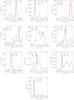 |
Fig. A.1
The mean 13CO spectra of the IRDCs of our sample. The spectra have been averaged over the AV > 7 mag box (see Sect. 3.2 for the detailed definition). The dotted vertical lines indicate the velocity interval chosen to represent the cloud. The red line shows a fit of a Gaussian to this velocity interval. The blue line shows another Gaussian fit, performed over the interval vpeak − 1.5σ,vpeak = 1.5σ where σ is the dispersion from the first Gaussian fit. The dispersions are shown in the panels. The third dispersion value, σd gives the standard deviation of the data within the chosen velocity interval. |
| Open with DEXTER | |
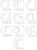 |
Fig. A.2
The same as Fig. A.1, but the spectra have been averaged over the Simon et al. (2006) ellipsoids (see Sect.3.2 for the detailed definition). |
| Open with DEXTER | |
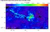 |
Fig. B.1
High-dynamic-range column density map of the cloud A, derived using a combination of MIR and NIR data. The green circle shows the largest ellipse from the Simon et al. (2006) catalog in the region. The white box outlines the region which was used alongside with the AV = 7 mag contour to define the region that is included in the analyses presented in Sect. 4. The contours are drawn at AV = [7,40] mag. The scale bar shows the physical scale assuming the distance as given in Table 1. |
| Open with DEXTER | |
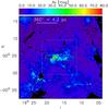 |
Fig. B.2
Same as Fig. B.1, but for the cloud B. |
| Open with DEXTER | |
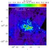 |
Fig. B.3
Same as Fig. B.1, but for the cloud C. |
| Open with DEXTER | |
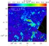 |
Fig. B.4
Same as Fig. B.1, but for the cloud D. The rectangular empty area results from missing NIR data. |
| Open with DEXTER | |
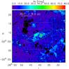 |
Fig. B.5
Same as Fig. B.1, but for the cloud E. |
| Open with DEXTER | |
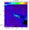 |
Fig. B.6
Same as Fig. B.1, but for the cloud F. The areas of missing data (marked with zeros) result from strong MIR nebulosity that hinders the MIR mapping technique. |
| Open with DEXTER | |
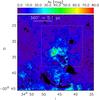 |
Fig. B.7
Same as Fig. B.1, but for the cloud G. |
| Open with DEXTER | |
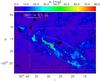 |
Fig. B.8
Same as Fig. B.1, but for the cloud H. |
| Open with DEXTER | |
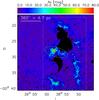 |
Fig. B.9
Same as Fig. B.1, but for the cloud I. The areas of missing data (marked with zeros) result from strong MIR nebulosity that hinders the MIR mapping technique. |
| Open with DEXTER | |
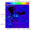 |
Fig. B.10
Same as Fig. B.1, but for the cloud J. The areas of missing data (marked with zeros) result from strong MIR nebulosity that hinders the MIR mapping technique. |
| Open with DEXTER | |
Appendix C: Response of the technique to changes of the opacity-law
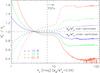 |
Fig. C.1
Response of the column densities derived using the combined NIR+MIR technique to
the adopted NIR-to-MIR opacity-law. The curves show the ratio of column densities
derived with alternative opacity-laws ( |
| Open with DEXTER | |


© ESO, 2012
Current usage metrics show cumulative count of Article Views (full-text article views including HTML views, PDF and ePub downloads, according to the available data) and Abstracts Views on Vision4Press platform.
Data correspond to usage on the plateform after 2015. The current usage metrics is available 48-96 hours after online publication and is updated daily on week days.
Initial download of the metrics may take a while.