| Issue |
A&A
Volume 548, December 2012
|
|
|---|---|---|
| Article Number | A105 | |
| Number of page(s) | 15 | |
| Section | Interstellar and circumstellar matter | |
| DOI | https://doi.org/10.1051/0004-6361/201219783 | |
| Published online | 30 November 2012 | |
Online material
Appendix A: Details on the fitting routine
For the determination of a fit curve to the color–magnitude data required for the subsequent search for excess sources, we used a polynomial fitting routine. We chose a polynomial degree n and then proceeded as follows:
-
1.
select only the single stars from the sample of all stars;
-
2.
perform a least-squares fit for polynomial of degree n;
-
3.
calculate χ2 goodness-of-fit;
-
4.
calculate
 for all stars;
 -
5.
remove stars with |σ′| > 3 from the sample;
-
6.
repeat from 2) until converged.
We did this for polynomials of increasing degree, starting with n = 1. For all colors, the quality of the fit does not increase significantly beyond n = 4, therefore we chose to use polynomials of fourth degree in all cases.
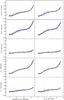 |
Fig. A.1
Obtained fits and error estimates for all three colors and additionally the Ks − [22] and Ks − [3.4] colors against absolute magnitude in the first WISE band and against V − Ks color. |
| Open with DEXTER | |
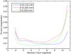 |
Fig. A.2
Inferred errors for our fits. As can be seen, the fit is very well constrained for intermediate M-dwarfs, but less constrained at both ends of the fit. At the high-luminosity end, we mitigate this problem by including several K-dwarfs. |
| Open with DEXTER | |
Polynomial fits.
From the χ2 value of the fit, it is possible to estimate the amount of intrinsic scatter in the stellar colors, assuming the error estimates for WISE are correct. As seen before, the WISE errors are likely to be overestimated because the χ2 values for all three fits are lower than one. We conclude that the intrinsic scatter is small and the actual deviations from the fit are dominated by measurement errors. This is true for all WISE colors ([3.4] – [12] , [3.4] – [22] and [12] – [22] ). The Ks − [22] , which we also investigated and show here for reference, has a higher χ2 value, and intrinsic scatter (induced by scatter in the Ks color) might play a more substantial role here. Ks − [3.4] is very good again, with a low χ2 value. We show it here for reference as well because it bridges the 2MASS longest and WISE shortest wavelengths for M-dwarfs, which we think could be useful.
While it is possible to obtain uncertainties on the derived parameters of a polynomial fit, this is of limited helpfulness because the individual parameters are highly correlated. To estimate the error on our fit, we again took a data-driven approach. We used the unmodified σ errors from WISE (not σ′) and produced 1000 data sets by randomly adding Gaussian errors with a standard deviation of σi to each measurement. We fit these 1000 data sets using our fitting routine. We then calculated the uncertainty of our fit at every point by calculating the standard deviation of these 1000 obtained polynomial fits.
Figure A.1 summarizes the fits and their upper and lower limits (dashed lines). Because the errors are small and hard to see in this representation, Fig. A.2 shows the error of each fit as a function of the absolute magnitude in the first WISE band. As can be seen, the errors are generally small, mostly below 0.02 mag, and thus much smaller than the measurement errors from the individual stars, which is why we did not provide an in-depth discussion of fitting errors in our analysis section (the error is not dominated by the fitting error). At both ends of the fit, the fitting errors naturally increase because the fact that the fit is less constrained at the ends. For the high-luminosity end of the M-dwarfs, this effect can be mitigated by including some K dwarfs, as we have done. We have good reasons to believe that our fundamental assumption that the colors can be fitted by a (fourth-order) polynomial holds reasonably well in the stellar regime (namely, the χ2 values of our fits are very good).
We summarize the parameters of our obtained fourth-order polynomials in Table A.1. The expected color can then be calculated as

with p being the proxy for the stellar temperature (either absolute 3.4 μm magnitude or V − Ks color). In addition to the three WISE bands, we also provide fits for the Ks − [22] color here. The Ks – [22] color can also be used for Spitzer data using the small offset of 0.083 mag determined in Fig. 2.
© ESO, 2012
Current usage metrics show cumulative count of Article Views (full-text article views including HTML views, PDF and ePub downloads, according to the available data) and Abstracts Views on Vision4Press platform.
Data correspond to usage on the plateform after 2015. The current usage metrics is available 48-96 hours after online publication and is updated daily on week days.
Initial download of the metrics may take a while.