| Issue |
A&A
Volume 546, October 2012
|
|
|---|---|---|
| Article Number | A28 | |
| Number of page(s) | 21 | |
| Section | Stellar structure and evolution | |
| DOI | https://doi.org/10.1051/0004-6361/201219528 | |
| Published online | 01 October 2012 | |
Online material
Appendix A: Chemical composition of explosion models
Tables A.1–A.3 show the chemical composition of the three explosion models we use (taken from Woosley & Heger 2007).
Chemical composition (mass fractions) of the 12 M⊙ model used.
Appendix B: Code updates compared to J11
B.1. Photoexcitation/deexcitation rates
Because the computations here are for earlier epochs than in J11, photoexcitation/deexcitation rates in the NLTE solutions have to be included. We therefore implemented a modified Monte Carlo operator to allow for partial deposition of photoexcitation energy along the photon trajectories. A photon packet of comoving energy E and frequency ν, coming into resonance with a transition l → u of atom k, where the upper level  (=the number of levels included in the NLTE solution of atom k), now increases the number of photoabsorbed packages by
  (B.1)where i is the zone index and
  the Sobolev optical depth. The packet then continues (undeflected) with energy
  . For lines with
  , we retain the treatment described in J11 (scattering/fluorescence is treated explicitly in the transfer). rescaled so that no photoexcitation energy is deposited).
The values for  should be chosen large enough to reasonably well sample the total number of photoexcitations from each level, but small enough to ensure stability and keep computation times limited (matrix inversion times in the statistical equilibrium solutions scale as cubed). The values used here can be found in Table B.2. We have chosen to set
  for all iron-group elements (except Fe i, Fe ii and Cr ii, where we solve for more levels), and
  for the non-iron-group elements.
In the Sobolev approximation, the photoexcitation rates to be used in the statistical equilibrium equations are given by (Castor 1970)  (B.2)\vadjust{\eject\vspace*{11cm}}where Blu is the Einstein coefficient for photoexcitation, βlu is the escape probability, and
  is the far blue-wing mean intensity (before Jν is affected by the line). The deexcitation rate is related by detailed balance
  (B.3)where gl and gu are the statistical weights.
Overlapping lines may cause  to significantly vary with the choice of the blue frequency. We therefore do not compute the photoexcitation rates from this equation, but by adding the contributions from Eq. (B.1). Since stimulated emission is treated as negative absorption in the Sobolev optical depth, Eq. (B.1) gives only the net number of photons absorbed in the line; absorptions minus stimulated emissions. The actual number of absorptions occurring is therefore higher by a factor (1 − glnu/gunl)-1, where nl and nu are the populations of levels l and u, so the estimator for the photoexcitation rate is
  (B.4)where Ni,k,l,u is the total number of packets absorbed in the transition in the Monte Carlo simulation.
For lines with  , we allow lasering to occur in the transfer by using the same formalism as for normal positive optical depths (Eq. (B.1)). In these cases we compute the deexcitation rate as
 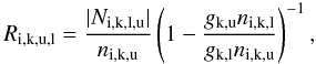 (B.5)and then use Eq. (B.3) to get the excitation rate.
B.2. Charge transfer
We now generalize the treatment of the O ii + C i → O i(2p(1D)) + C ii reaction in J11, by assuming that all charge transfer reactions occur to the state (either in the recombining or in the ionizing element) that gives the smallest energy defect.
B.3. Photoionization rates and photoelectric heating rates
We have also modified the estimators for the photoionization rates and the photoelectric heating rates. Whereas the previous treatment did not allow splitting of packets upon continuum interaction, a photon packet passing a region of optical depth τ, of which photoionization by atom k, level l, contributes  , now adds a contribution
 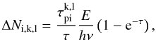 (B.6)to the number of photons Ni,k,l absorbed in the corresponding continuum. The heating rate is increased by
 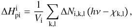 (B.7)where Vi is the volume of the zone, and χk,l is the ionization potential.
B.4. Electron scattering
We implement electron scattering in the following way. The total continuum optical depth to the next point of interest (a zone boundary, a line, or a photoionization threshold) is 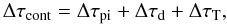 (B.8)where Δτpi is the photoionization optical depth, Δτd is the dust optical depth, and ΔτT is the Thomson optical depth. The fraction of photons absorbed in photoionization continua is
 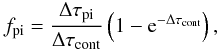 (B.9)the fraction absorbed by dust is
 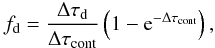 (B.10)the fraction that Thomson scatter is
 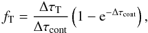 (B.11)and the fraction that do not interact is
 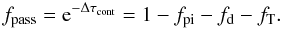 (B.12)We let the fractions fpi and fd be absorbed in photoionization continua and by dust, respectively. We then let the remaining fraction (fT + fpass) Thomson scatter with probability
  (B.13)and continue through with probability 1 − pT. If Thomson scattering occurs, we draw a position for the scattering from
  (B.14)and a new direction cosine μ from
  (B.15)where z is a uniform random number between 0 and 1, and p(μ′) is the Rayleigh phase function
  (B.16)We treat the scattering as coherent in the fluid frame, i.e. we ignore the small energy shifts occurring due to the thermal motions of the electrons, as well as the Compton shift.
Transitions into which (part of the) Lyα flux is allocated.
B.5. Line overlap
When the density is high, the line escape probabilities may be enhanced from their Sobolev values βS by overlapping continua and lines, so that  (B.17)We take the βC term into account as described in J11. In this paper, we also take the βL term into account for Lyα and Lyβ, which are important for the spectral formation in Type II SNe.
Lyα reaches optical depths as high as τS = 1010−1011 in the early nebular phase, and may branch into several iron-group lines around 1215.67 Å before escaping the resonance layer. Preliminary simulations (which we hope to expand on in a future publication) show that at typical conditions in the early nebular phase, the branching probability is  (B.18)Here we use
  . We assume that the absorbing lines are the ones which, at 300 days in the core H region, are optically thick and within 100 Doppler widths (on the red side) of the Lyα rest wavelength, with allocation to these transitions in equal proportions. The lines, which fall in the 1215.67−1220 Å range, are listed in Table B.1.
Model atoms used.
The O i λ1025.76 2p4(3P) − 3d(3Do) transition lies within the Doppler core of Lyβ. If the O i λ1.129 μm 3p(3P) − 3d(3Do) transition is optically thin, and complete l-mixing in both H i n = 3 and O i 3d3D is assumed, the branching probability for O i fluorescence is7 (B.19)where n(O i) and n(H i) are the number densities of O i and H i. At solar metallicity n(O)/n(H) = 4.9 × 10⁻⁴, so
  = 2.1 × 10⁻⁵, which is the value we use.
B.6. Photoionization cross sections
For excited states with unknown photoionization cross sections, we use the hydrogenic approximation (Rybicki & Lightman 1979)  (B.20)where
  is the ionization threshold, gk,l is the Gaunt factor (which we set to unity for all levels), Zk is the effective nuclear charge (number of protons minus number of screening electrons), and nk,l is the effective principal quantum number
  (B.21)where Ek,l is the level energy and χk,0 is the ground state ionization potential.
We use a threshold for how many levels to compute photoionization cross sections for. For this paper this limit was set to 50 levels. Tests showed that contributions by levels above this were small for all epochs modeled.
B.7. Free-bound emissivities
For hydrogen, we use detailed emissivity functions obtained by applying the Milne relations to the photoionization cross sections, which we obtain from Verner et al. (1996) for n = 1, and Bethe & Salpeter (1957) for n = 2. For n = 3 and higher we use the hydrogenic approximation.
For all other atoms k we use a simplified prescription, where recombination to level l gives an emissivity of 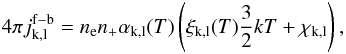 (B.22)is emitted over a box-shaped profile between 0.5−1.5 kT. Here αk,l(T) is the specific recombination coefficient, and ξk,l(T) is taken as 0.55 for all atoms, levels, and temperatures, the value for hydrogen at a few thousand K (Spitzer 1948).
B.8. Collision strengths
For transitions with unknown collision strengths we use van Regemorter’s formula (van Regemorter 1962) for allowed lines (taken as fosc > 10-3), and 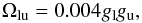 (B.23)for forbidden lines (Axelrod 1980).
B.9. Model atoms
Table B.2 lists the model atoms used. Compared to J11, we now include more levels in the NLTE solutions, and have also added Fe iii and Co iii8. We have added collision strengths for Ni ii (Cassidy et al. 2010, 2011, we use the values at 5000 K). The sources for the rest of the atomic data are given in J11.
© ESO, 2012
Current usage metrics show cumulative count of Article Views (full-text article views including HTML views, PDF and ePub downloads, according to the available data) and Abstracts Views on Vision4Press platform.
Data correspond to usage on the plateform after 2015. The current usage metrics is available 48-96 hours after online publication and is updated daily on week days.
Initial download of the metrics may take a while.