| Issue |
A&A
Volume 546, October 2012
|
|
|---|---|---|
| Article Number | A60 | |
| Number of page(s) | 16 | |
| Section | Interstellar and circumstellar matter | |
| DOI | https://doi.org/10.1051/0004-6361/201219006 | |
| Published online | 05 October 2012 | |
Online material
Appendix A: The Kelvin Helmholtz instability in stratified flows
A.1. Linear theory (Chandrasekhar 1961)
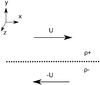 |
Fig. A.1
Configuration of the stratified flow. |
| Open with DEXTER | |
A flow can be considered as incompressible with respect to the
Kelvin-Helmholtz-instability if the Mach number of the velocity discontinuity
ℳcd = Δv/ cs ≲ .3
where Δv is the velocity difference at the interface and
cs the sound speed. At the centre of the binary system,
the winds are subsonic and the flow is incompressible as the two winds collide
head-on. We use the incompressible approximation in the following computations.
However, this may not be fully applicable further away from the binary as the winds
re-accelerate. That said, the interface remains marginally sonic
( in all our simulations). In this case, the evolution of the KHI is complex to
determine as it depends on the binary parameters (η,
β) but also on the development of the KHI closer to the binary. We
have a system with a mean profile
U = ± Uex.
Above y = 0, the flow has a density ρ+
and ρ− for
y < 0 (see Fig. A.1). We neglect the Coriolis force since the local shear timescale
τS = Δx/ ΔU ~ 10-6 yr
is much shorter than the orbital period
τΩ ~ 10-1 yr. In this approximation, the
linearised equation of motion is:
in all our simulations). In this case, the evolution of the KHI is complex to
determine as it depends on the binary parameters (η,
β) but also on the development of the KHI closer to the binary. We
have a system with a mean profile
U = ± Uex.
Above y = 0, the flow has a density ρ+
and ρ− for
y < 0 (see Fig. A.1). We neglect the Coriolis force since the local shear timescale
τS = Δx/ ΔU ~ 10-6 yr
is much shorter than the orbital period
τΩ ~ 10-1 yr. In this approximation, the
linearised equation of motion is: 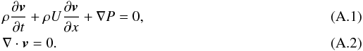 In
the following, each quantity is Fourier transformed in x
and t thanks to homogeneity:
Q = Qexp [i(ωt − kx)].
Rewriting the equation of motions and combining them leads to
In
the following, each quantity is Fourier transformed in x
and t thanks to homogeneity:
Q = Qexp [i(ωt − kx)].
Rewriting the equation of motions and combining them leads to 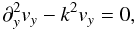 (A.3)which is solved
with two decaying solutions
(A.3)which is solved
with two decaying solutions 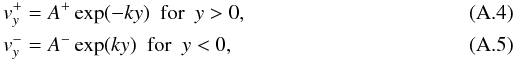 A+
and A− being two arbitrarily chosen constants that are
adjusted by jump conditions at the interface y = 0: pressure should
be continuous and fluid particles should stick to the interface on both sides. The
pressure condition is given by:
A+
and A− being two arbitrarily chosen constants that are
adjusted by jump conditions at the interface y = 0: pressure should
be continuous and fluid particles should stick to the interface on both sides. The
pressure condition is given by: 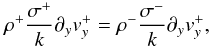 (A.6)where
σ ± = ω ± U. The
second condition is obtained defining a displacement vector
ξ(x) that follows the interface. By definition, a
fluid particle located at
(x,ξ(x) − ϵ) satisfies
(A.6)where
σ ± = ω ± U. The
second condition is obtained defining a displacement vector
ξ(x) that follows the interface. By definition, a
fluid particle located at
(x,ξ(x) − ϵ) satisfies
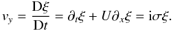 (A.7)Applying this
to both side of interface (± ϵ) leads to the jump condition
(A.7)Applying this
to both side of interface (± ϵ) leads to the jump condition
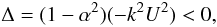
 (A.8)Combining (A.6) and (A.8) and looking for non trivial solutions gives
 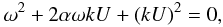 (A.9)where
α = (ρ+ − ρ−)/ (ρ+ + ρ−).
An instability arises whenever
(A.9)where
α = (ρ+ − ρ−)/ (ρ+ + ρ−).
An instability arises whenever
 (A.10)which is always
true since −1 ≤ α ≤ 1. The growth rate
is
(A.10)which is always
true since −1 ≤ α ≤ 1. The growth rate
is 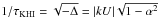 .
Hence, a density contrast |α| close to 1 strongly dampens the
growth rate of the KHI.
.
Hence, a density contrast |α| close to 1 strongly dampens the
growth rate of the KHI.
In colliding wind binaries, the density and the velocity of both winds are related
through the momentum-flux ratio η. Using Eq. (1) and mass conservation for both winds
then and assuming the interaction occurs far enough from the binary (so that
r1 ≃ r2), the density ratio
is roughly 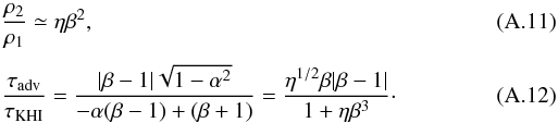
A.2. Nonlinear evolution
A.2.1. Two-dimensional evolution
 |
Fig. A.2
Snapshot of the mixing at t = 21 (in dimensionless units) for α = 0.5. |
| Open with DEXTER | |
To investigate the evolution of the KHI in the nonlinear regime, we performed numerical simulations for increasing α. The 2D setup is as follows: box size (lx = 8,ly = 4), resolution (1024 × 256), code PLUTO (Mignone et al. 2007), adiabatic equation of state P ∝ ρ5/ 3, background pressure P = 1 in the initial state (using units scaled to the box length, density, and velocity shear). Reflective boundary conditions are enforced in y to confine the instability in the simulation box. We always have ρ+ > ρ− i.e. the densest medium is found where y > 0.
In addition to that, we follow the mixing using a passive scalar as explained in
Sect. 2.3. We performed simulations for
{α = 0,0.5,0.9,0.99} .
Kelvin-Helmholtz eddies are clearly present in the density snapshot shown in
Fig. A.2 for model α = 0.5.
To show the diffusion of the passive scalar as a function of time, we plot the
evolution of  as a function of y and t in Fig. A.3. These results demonstrate that when
α ≠ 0, the scalar diffusion propagates much less in the denser
medium (y > 0) and that diffusion looks
less efficient when |α| increases, in the sense that the region
with intermediate values of the scalar s becomes smaller when
α increases.
as a function of y and t in Fig. A.3. These results demonstrate that when
α ≠ 0, the scalar diffusion propagates much less in the denser
medium (y > 0) and that diffusion looks
less efficient when |α| increases, in the sense that the region
with intermediate values of the scalar s becomes smaller when
α increases.
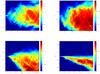 |
Fig. A.3
Mixing due to the KHI. From left to right, top to bottom: α = 0,0.5,0.9,0.99. |
| Open with DEXTER | |
A.3. Three-dimensional evolution
We performed simulations for α = 0 and 0.9 in 3D to compared them to
the 2D ones. They are very similar to the 2D configuration, except for the resolution,
which was reduced to 500 × 100 × 100 in order to reduce computational costs. We set
lz = lx = 4.0,
where  is shown in Fig. A.4. The direct comparison with the 2D cases
indicates that faster diffusion into the more tenuous region still occurs in the 3D
simulation.
is shown in Fig. A.4. The direct comparison with the 2D cases
indicates that faster diffusion into the more tenuous region still occurs in the 3D
simulation.
Figure A.5 shows the mixing at different times in the 2D and 3D simulations, for α = 0.,0.9. It confirms that both in the 2D and 3D case, the KHI behaves similarly with respect to the velocity gradient.
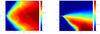 |
Fig. A.4
Mixing in the 3D simulations with α = 0 (left) and α = 0.9 (right). |
| Open with DEXTER | |
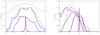 |
Fig. A.5
Mixing in 2D simulations (blue solid line) and 3D simulations (red dashed line) for α = 0 (left panel) and α = 0.9 (right panel). The different curves show different timesteps separated by Δt = 5. |
| Open with DEXTER | |
Appendix B: Parameters of the simulations
Parameters of the simulations.
© ESO, 2012
Current usage metrics show cumulative count of Article Views (full-text article views including HTML views, PDF and ePub downloads, according to the available data) and Abstracts Views on Vision4Press platform.
Data correspond to usage on the plateform after 2015. The current usage metrics is available 48-96 hours after online publication and is updated daily on week days.
Initial download of the metrics may take a while.