| Issue |
A&A
Volume 541, May 2012
|
|
|---|---|---|
| Article Number | A91 | |
| Number of page(s) | 28 | |
| Section | Interstellar and circumstellar matter | |
| DOI | https://doi.org/10.1051/0004-6361/201118218 | |
| Published online | 04 May 2012 | |
Online material
Appendix A: Details of the models and benchmark tests
The purpose of this appendix is twofold. First, it presents details of the implementation of the model and second, it compares of results with other codes and benchmark problems. The model is based on those of Bruderer et al. (2009b,a, 2010) and Bruderer (2010), although it contains several improvements. The structure of the model is summarized in Fig. A.1. The modeling process starts with a gas and density distribution e.g. obtained from an analytical prescription. Different modules then calculate the dust temperature and UV radiation (Sect. A.2), abundances of atomic or molecular species (Sect. A.3), and the level population of molecules or atoms acting as coolants (Sect. A.4). The gas-temperature is then calculated from the balance between heating and cooling processes (Sect. A.5). As the abundance and level population enter the heating and cooling rates, abundances and level populations need to be re-calculated until convergence. Finally, spectral lines can be calculated and compared with observations.
To carry out the calculation, the modeled region is divided into individual cells. In this present study, we assume a axisymmetric structure. Since all geometric information is contained in one separate module, the code can in principle also be run for spherically symmetric or three-dimensional structures.
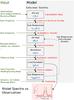 |
Fig. A.1
Modeling flowchart. |
| Open with DEXTER | |
The current study applies the model to a protoplanetary disk, but the model can also be used in the context of protostellar envelopes, for example to calculate the molecular emission from UV irradiated outflow walls. For future applications, we thus present all modules in this appendix, even though they are not used in the current work (such as the calculation of the dust temperature).
A.1. Dust radiative transfer
A.1.1. Dust temperature
The dust temperature in steady state is obtained from the equilibrium between energy absorbed and emitted by dust 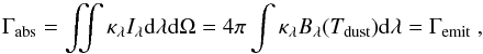 (A.1)where the dust opacity per unit mass is κλ, the incident radiation field is Iλ, and the Planck function for the dust temperature is Bλ(Tdust). The radiation field consists of contributions from both the stellar radiation field and the ambient radiation by dust emission. Thus, different positions in the model are coupled by means of the radiative transfer equation. We neglect the “back-warming” of dust by hot gas and further assume a unique dust temperature for different sizes of dust.
In this present study, we implement the Monte Carlo technique proposed by Bjorkman & Wood (2001): photon packages with an energy distribution following the stellar radiation field are propagated until interaction (scattering or absorption followed by re-emission). Scattering only changes the direction of a photon package. To sample the scattering angle, we use a Henyey-Greenstein function, which defines the scattering angle by only one parameter, g = ⟨ cos(θ) ⟩ . Absorption increases the amount of energy deposited into a cell. For a cell of dust mass M, the dust temperature Tnew after absorption of Ni photon packages is given by 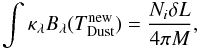 (A.2)with the energy per photon package δL = L/N, where the stellar luminosity L is divided by the total number of photon packages N. When an absorption event increases the local temperature by
  , the photon-package is re-emitted at a wavelength given by (Baes et al. 2005)
 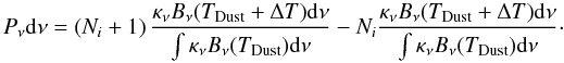 (A.3)This probability distribution function (PDF) accurately corrects for the incorrect spectrum of previously reemitted photons (at a too low temperature). However, it can sometimes become negative. In such cases, the approximative PDF given in Bjorkman & Wood (2001) is used. This procedure is generally very efficient as it does not require any global iteration and the dust temperature increases to the correct value. In regions of very high optical depth, however, photons can get stuck owing to a very high number of absorption and re-emission processes. We thus implement the diffusion approximation derived in Robitaille (2010), based on Min et al. (2009). Regions of very low optical depth can suffer too little absorption resulting in a noisy dust temperature (see e.g. Bruderer 2010, Fig. D.2). We implement a method proposed by Pinte et al. (2006) and measure the ambient radiation field using the estimator given in Lucy (1999) during the propagation of the photons. After all photons have propagated, the dust temperature can be improved using this value.
To benchmark the dust temperature calculation, we use the benchmark problems proposed in Ivezic et al. (1997) and compare our results with calculations obtained with the DUSTY code (Ivezic & Elitzur 1997). The benchmark problem consists of a spherical cloud with two different density gradients (either ∝ r-2 or constant) and four different total radial optical depth at 1 μm (τ1 μm = 1,10,100, or 1000). The input spectra is a black body and the dust properties follow a simple analytical law. Scattering is assumed to be isotropic. The agreement between the codes is perfect, being closer than about a percent.
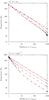 |
Fig. A.2
Results of a spherical benchmark test for the dust temperature calculation (Ivezic et al. 1997). The dust temperature obtained from this work is given by a red line, while the results from DUSTY are given by black signs. The solid line corresponds to τ1μm, and the dashed, dotted, and dash-dotted lines to τ1 = 10,100, and 1000, respectively. a) Constant density, b) density ∝ r-2. |
| Open with DEXTER | |
As a second benchmark problem, we calculate the dust temperature in a protoplanetary disk with very high total optical depth (Pinte et al. 2009). We calculate their benchmark problem for isotropic scattering with a midplane optical depth at 0.86 μm of τ = 103 and 105 (their Fig. 9). In Fig. A.3, we show the midplane temperature for the two models compared to the results obtained with MCFOST. The agreement is very good for the model with τ = 103. For the run with τ = 105, the agreement is again very good with deviations smaller than a few percent, even in the region shadowed by the dense inner rim. These deviations are comparable to those between the other codes participating in that benchmark study.
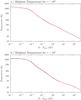 |
Fig. A.3
Dust temperature at midplane for the disk benchmark problem (Pinte et al. 2009). The result from our code is given in red, the result from MCFOST (Pinte et al. 2006) in black. |
| Open with DEXTER | |
A.2. UV field
Since the calculation of the dust temperature does not explicitly compute the radiation field as a function of wavelength, the intensity at UV and optical wavelengths is calculated in a second step. This intensity is used for example to calculate photodissociation rates. The calculation of the intensity uses the same method for the propagation of the photon packages as the calculation of the dust temperature. The radiation field is then calculated with the method proposed by van Zadelhoff et al. (2003). For each wavelength bin, N photon packages are propagated. All photon packages are assigned with an initial intensity Iλ(0) = FλS/N, where Fλ is the input flux and S the surface it passes through. This intensity then drops to Iλ(s + Δs) = Iλ(s)e−Δτλ, when the package advances by Δs with an optical depth Δτλ. The mean intensity is calculated from 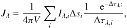 (A.4)with the volume of the cell V and the sum taken over all photon packages passing through a cell. The distance and optical depth as an individual photon package i passes through a cell are given by Δsi and Δτλ,i. Since we calculate the mean intensity for a few wavelengths only, the input intensity is obtained by averaging over the input (stellar) spectra in each individual spectral band. Photons from the interstellar radiation field (Draine 1978) are also accounted for.
As a benchmark test, we calculate the mean intensity in a spherical cloud, switching scattering off. We compare the calculated intensity to the analytically obtained intensity and find agreement to better than one percent. The implementation of the scattering follows the calculation of the dust temperature and was tested in the previous paragraph.
A.3. Chemistry
Abundances of molecular and atomic species are obtained from the solution of the rate equations 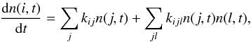 (A.5)with the abundance n(i,t) (cm-3) of a species i at time t. The rate of destruction and formation of a species is given by the coefficients kij and kijl, respectively. In addition, three-body reactions can be entered, but our current network does not contain any. The set of coupled, stiff, and non-linear differential Eqs. (A.5) is solved by the DVODE solver (Brown et al. 1989) for the temporal evolution of the species. We verify that the solution complies with the conservation of elements and charge. We note that the DVODE solver is widely used for applications in astrochemistry and well-tested (e.g. Nejad 2005). To obtain steady-state abundances, Eq. (A.5) is solved for dn(i,t)/dt = 0 using a globally convergent Newton-Raphson method. To close the system of equations Eq. (A.5), some rate equations are replaced by conservation equations. If the steady-state solver fails to converge, the abundances are obtained from the time-dependent solver running to a high chemical age (>10 Mio. years).
To test numerical aspects of the solver, we calculate abundances in an isothermal slab of constant density with UV irradiation. A small chemical network from the PDR comparison study by Röllig et al. (2007) is used for this test. We first calculate their problem F4 (for a density of 105.5 cm-3, UV field of χ = 105, and a temperature of 50 K) with the steady-state solver. In Fig. A.4, we give the abundances of H, H2, O, O2, C+, CO, and electrons and compare them to the results obtained from PDR codes. Our code to within their scatters agrees with the other codes. The scatter in the H2 abundance is due to a different implementation of some reactions, such as H2 dissociation including self-shielding. We also calculated the abundances with the time-dependent solver running to an old chemical age and found an agreement to better than a factor of 10-4 with the steady-state solution.
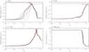 |
Fig. A.4
Result of the chemistry benchmark for a slab with UV irradiation (Röllig et al. 2007, problem F4). The result of our code is given by the red line, the results of the PDR codes by gray lines. |
| Open with DEXTER | |
A.3.1. Chemical network
The chemical network used in our work contains 10 elements, 109 species, and 1492 reactions. We use the same elemental composition as Jonkheid et al. (2006) and Woitke et al. (2009a), which is summarized in Table A.1. The species contained in the network are given in Table A.2. We note that  is vibrationally excited H2. PAH0, PAH+, and PAH− are neutral, positively, and negatively charged PAHs respectively and PAH:H denotes hydrogenated PAHs. Species frozen-out onto dust grains are shown by JX, for example JCO is CO frozen-out.
Elemental composition. a(b) means a × 10b.
The chemical reaction network is based on the studies by Doty et al. (2004), Stäuber et al. (2005), and Bruderer et al. (2009b), but contains some extensions. The following reaction types are included:
1.) H2 formation on dust
For the formation of H2 on dust grains, we implement the rate by Sternberg & Dalgarno (1989), scaled to the appropriate grain size. We use the sticking coefficients of Cuppen et al. (2010). Since the gas/dust ratio can vary over a model, rates involving small dust are scaled to the local gas/dust ratio.
2.) Freeze-out, thermal, and non-thermal desorption
Freeze-out and thermal or non-thermal desorption are implemented following Visser et al. (2009b) and references therein. The thermal desorption rates account for the abundance of the ice on the surface and change from zeroth to first order behavior when the ice contains less than a monolayer of ice. As in Visser et al. (2009b), we use the same pre-exponential factor for all species except for H2O (Fraser et al. 2001) and CO (Bisschop et al. 2006). Binding energies follow Aikawa et al. (1997) and Sandford & Allamandola (1993).
Non-thermal evaporation by UV photons or cosmic-rays depends on a yield indicating the number of molecules desorbed per grain per incident UV photon. We assume the same yields used by Visser et al. (2009b), following Öberg et al. (2007, 2009b). To simulate cosmic-ray induced desorption, a small background UV flux corresponding to 104 photons cm-2 s-1 (Shen et al. 2004) is added to the stellar UV flux.
3.) Hydrogenation of simple species on ices
In addition to freeze-out and evaporation, we implement the grain-surface hydrogenation of simple species. We follow the approach of Visser et al. (2011) and Hollenbach et al. (2009). The hydrogenation leads to saturation of species frozen-out, from JC → JCH → JCH2 → JCH3 → JCH4, JN → JNH → JNH2 → JNH3 and JO → JOH → JH2O. Other grain-surface reactions to build up more complex species are not accounted for, but the focus of our work is on simple species.
5.) Gas-phase reactions
Most reactions in our network (1132 out of 1492) are pure gas-phase reactions, such as ion-neutral, neutral-neutral, or charge exchange reactions. Our network contains all reactions from the UMIST 2006 database (Woodall et al. 2007) involving the species given in Table A.2. Details of the implementation are given in Bruderer et al. (2009b).
6.) Photodissociation
Photodissociation rates are calculated from the local radiation field using the cross-sections for discrete and continuous absorption given by van Dishoeck (1988), van Dishoeck et al. (2006), and van Hemert & van Dishoeck (2008)3. For the dissociation of H2, CO, and the ionization of C, we include the effects of self-shielding by reducing the unshielded rate with a self-shielding factor. For H2, the factor given in Draine & Bertoldi (1996) is used. For CO, we implement the factors given in Visser et al. (2009a) and for C, the factor of Kamp & Bertoldi (2000) is used. We however limited the shielding of C by H2 to 0.5, owing to the overlap of H2 lines with the wavelengths at which carbon is photoionized.
The self-shielding rates depend on the column densities of H2, C, and CO towards the UV source. We calculate these column densities together with the UV field (Sect. A.2) by averaging over the densities of all photon packages passing through a cell, weighted by their intensity.
7.) X-ray induced processes
As demonstrated by Bruderer et al. (2009b), the influence of X-rays on the chemistry can be accurately approximated by secondary ionizations induced by fast photo-electrons from H2 and H ionization. We follow their approach and calculate the X-ray ionization rate using the cross-sections given in their Appendix A. The rates for the secondary processes are taken from Stäuber et al. (2005). We note that the cosmic-ray-induced photodissociation rates are scaled-up to the X-ray ionization rate following Stäuber et al. (2005).
8.) Cosmic-ray-induced reactions
Rates for direct cosmic-ray-induced ionization processes are taken from the UMIST 2006 network. Cosmic-ray-induced photoionization rates are also taken from that database, with the exception of CO, H2, and H, where we follow Stäuber et al. (2005). For the CO dissociation, we use the rates of Gredel et al. (1987) implemented with the fitting equation provided in Maloney et al. (1996). We account for the ionization of CO, H2, and H by the decay of excited He (21P state, 19.8 eV, see Yan 1997).
9.) PAH/small grain charge exchange/hydrogenation
We assume that PAHs and small grains are well-mixed with the gas and thus not scaled to the gas/dust ratio. For the photoionization, charge-exchange, and recombination, we use the rates given in Wolfire et al. (2003) with a collision rate parameter φpah = 0.5. For species heavier than hydrogen, the recombination rates are scaled to  , where mamu is the mass of the molecule.
The formation of CH+ and H2 on PAHs is implemented using the rates of Jonkheid et al. (2006). We include the reactions 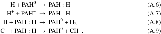 Reactions (A.6)–(A.8) run at 10-9 cm3 s-1, while (A.9) runs at the same speed as the recombination of C+ with PAH0.
10.) Reactions with  (excited state H2)
Vibrationally excited H2 is included into the chemistry with a two-level approximation. denotes H2 in a vibrationally excited pseudo-level with an energy corresponding to 30 163 K (London 1978). The energy stored in the vibrational state can be used to overcome an activation barrier (e.g. Sternberg & Dalgarno 1995). Following Tielens & Hollenbach (1985), the rate coefficients of a species with can be approximated using the rate for H2 by reducing the exponential factor by 30 163 K. For a H2 rate ∝ exp(− γ/Tkin), the exponential factor for is thus γ ∗ = max(0,γ−30 163K). This approximation however overestimates the rate coefficients, if γ is too large and we switch off reactions with γ > 20 000 K.
The population of is determined by collisions with H and H2 (Tielens & Hollenbach 1985), spontaneous decay (2 × 10⁻⁷ s-1; London 1978) and the pumping by FUV photons, which is assumed to be ten times the photodissociation rate.
A.4. Molecular/atomic excitation
The population ni (in cm-3) of a level i of a molecular or atomic species is determined by the rate equation 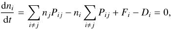 (A.10)with the rate coefficients for the transition between level i and j,
 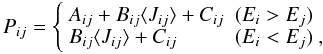 (A.11)with the level energy Ei, the collisional rate coefficients Cij and the Einstein A and B-coefficients Aij and Bij, respectively. The rate of chemical formation of a molecule forming into the state i and destroyed from that state is given by Fi and Di, respectively (Stäuber & Bruderer 2009). In the following, we assume steady-state conditions and set dni/dt = 0. To calculate the ambient radiation field
  (A.12)the normalized line profile function φij(ν) and the intensity depending on the frequency and direction is needed in every cell of the model. The intensity along a ray and for one frequency is calculated from the radiative transfer equation
  (A.13)with the absorption and emission coefficient αν and jν, respectively and the distance ds that the ray propagates. Both coefficients contain contributions from both line and dust absorption and emission. Since the level population enters the absorption and emission coefficients, Eqs. (A.10), (A.12), and (A.13) form a coupled problem, which is computationally very demanding to solve (see for example Hogerheijde & van der Tak 2000; Brinch & Hogerheijde 2010).
In this work, we employ an approximation similar to the escape probability method (e.g. van der Tak et al. 2007). In this approximation, the physical conditions and thus the source function Sν = jν/αν is assumed to be constant in the modeled region. The ambient radiation field ⟨ Jij ⟩ can then be expressed by an analytical expression, which greatly facilitates the calculation. For our models with physical conditions strongly varying with position, the approximation of a single zone with constant physical conditions is not applicable. The solution of Eq. (A.13) then reads  (A.14)using the definition of the optical depth, dτν = ανds and the background intensity Iν,bg. Similar to Poelman & Spaans (2005), we solve for the excitation at every position, although we approximate the local radiation field by keeping the source function constant along a ray. The time-consuming integration in Eq. (A.14) reduces in this way to a simple calculation of the opacity along a ray from the current position to the edge of the modeled region. This approximation allows us to solve for the excitation of complex problems (many lines, high optical depth) in a short time. For example the excitation of water in the models presented in this work can be solved in a few minutes using a standard PC.
To include pumping by dust and the velocity structure, we follow the approach of Takahashi et al. (1983). For the dust and line opacity τν,L and τν,D, along a ray, we calculate  The level population is then obtained from Eq. (A.10) with
 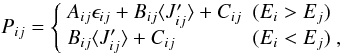 (A.17)and
 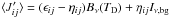 . The local dust temperature is given by TD and the background radiation (CMB) is given by Iν,bg. For the calculation of ϵij and ηij, either 6 or 26 directions and of order 40 frequency bins per line are used.
Once the level population is determined, the molecular cooling rate can be calculated and synthetic maps can be derived by solving the radiative transfer equation (Eq. (A.14)). Our raytracer produces images in fits format. To properly resolve the inner structure (hot core or inner disk), we shoot several rays per pixel through that region and average over the intensity. Along the ray, the integration steps within one computational cell are refined, according to the velocity structure in order to properly resolve narrow lines.
Benchmark test
To benchmark the excitation calculation, we calculate the problem proposed by van Zadelhoff et al. (2002), which consists of the calculation of the HCO+ excitation in a spherical, infalling class 0 cloud core. The physical conditions are given in Fig. A.5. The abundance of HCO+ is fixed to either 10-8 or 10-9 relative to the H2 density. The difficulty of this benchmark problem lies in the high optical depth reached in the lines and that collision partner densities are below the critical density. The level population is thus far from the local thermal equilibrium and radiative excitation is important.
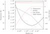 |
Fig. A.5
Physical conditions of the cloud core used to benchmark the excitation calculation. |
| Open with DEXTER | |
In Fig. A.6, we compare the solution obtained with this method with the solution calculated by RATRAN (Hogerheijde & van der Tak 2000). That code is widely used and has been well-tested against other codes. For an abundance of 10-9, the normalized level population agrees to within 30% with the solution provided by RATRAN. An exception is the J = 3 level in the inner part of the cloud. The deviations are larger for an abundance of 10-8, but still mostly within 30%. The intensity is obtained with the raytracer implemented in our code and convolved to the telescope beam. In Fig. A.6, the J = 1 → 0 and J = 4 → 3 lines are shown for a beam of 29′′ and 14′′, respectively. We also indicate the intensities obtained assuming local thermal equilibrium (LTE) and “thin” conditions, setting the ambient radiation field to 0. As the level populations, the line fluxes mostly agree to within about 30% of the intensity obtained with RATRAN. We note that the intensities obtained with RATRAN are calculated with their raytracer (SKY) and convolved using the MIRIAD package (Qi 2005). Thus, this benchmark problem also tests our raytracer and convolution routine.
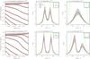 |
Fig. A.6
Result of the benchmark of the excitation calculation. The upper panel shows the results for a HCO+ abundance of 10-9 relative to H2, the lower panel for an abundance of 10-8 relative to H2. The plots on the left display the normalized level population of the first eight levels, the plots on the right show beam-averaged intensities. The black lines give results obtained using the RATRAN code, and the red dots/lines show results derived by this work. The gray shaded area indicates a 30% range to the RATRAN solution. |
| Open with DEXTER | |
The agreement found in with this benchmark problem is similar to the findings of Woitke et al. (2009b), who calculated the water emission from a Herbig Ae disk calculated with a similar method and compared them to RATRAN. We consider the agreement as reasonable and sufficient for our application, since the uncertainties entering through the chemical network calculation are much larger. It also shows that this method is a much better approximation than e.g. assuming LTE.
A.5. Thermal balance
The gas temperature is obtained from the equilibrium between the heating and cooling rates 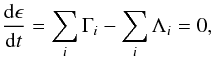 (A.18)where ϵ is the internal energy of the gas and Γi and Λi are different heating and cooling rates (for example, line cooling or photoelectric heating on dust grains). This non-linear equation is solved by a secant method starting from the dust temperature. If the convergence is insufficient, the process is restarted with a different value. Convergence is reached if the heating and cooling rate agree to within a predefined threshold in all cells (typically 1%). We implement the following heating and cooling rates (see Bruderer et al. 2009a):
1.) Photoelectric heating
Photoelectric heating on large graphite and silicate grains is implemented following Kamp & van Zadelhoff (2001). The required grain absorption cross-section, averaged over the FUV band, is taken to be consistent with the calculation of the UV field and the dust temperature. As for the chemistry, the rates involving dust grains are scaled to the local gas/dust ratio. Photoelectric heating on small dust grains is implemented following Bakes & Tielens (1994). We also implement their recombination cooling rate.
2.) Gas-grain heating or cooling
Depending on the difference between gas and dust temperature, gas-grain collisions can either heat or cool the gas. In regions of very high density, gas-grain collisions couple the gas temperature to the dust temperature (e.g. Doty & Neufeld 1997). We implement the heating and cooling rates following Young et al. (2004).
3.) H2 heating
Molecular hydrogen can contribute to the heating and cooling in different ways: (i) Line cooling. (ii) Heating through collisional deexcitation of FUV pumped H2. (iii) Formation heating. (iv) Photodissociation heating. For (i) and (ii), we use the analytical fit of Röllig et al. (2006) to the exact multilevel treatment by Sternberg & Dalgarno (1995). For (iii), we follow Kamp & van Zadelhoff (2001) and assume that one third of the binding energy of ~4.5 eV is released to the gas for heating. Photodissociation (iv) carries away about 0.4 eV in the form of heat to the gas (e.g. Jonkheid et al. 2004). We note that the H2 dissociation rate is taken to be consistent with the chemistry.
4.) Cosmic-ray heating
Following Cravens & Dalgarno (1978) and Glassgold & Langer (1973), a cosmic-ray ionization of H2 (H) releases 8 eV (3.5 eV) to the gas.
5.) X-ray heating
We implement the X-ray heating rates following Dalgarno et al. (1999) for a H2, H, and He mixture. The energy deposition rate per particle Hx is calculated using the cross-sections provided in Bruderer et al. (2009b).
6.) Line cooling (molecular and atomic fine-structure lines)
Cooling rates of molecular lines and atomic fine-structure lines are derived from the level population calculation (Sect. A.4). We account for O, C, C+, CO, 13CO, H2O, and OH. The abundance of 13CO is obtained from scaling the CO abundance by 12C/13C = 70 (Wilson & Rood 1994). Molecular data are taken from the LAMDA database (Schöier et al. 2005) and include the collisional excitation with H, H2, and electrons for O, C, and C+, respectively. For the molecular species, only excitation with H2 is available.
7.) Hydrogen Lyα and [O I] 6300 Å cooling
Hydrogen Lyα cooling and cooling by neutral oxygen [O i] by means of the metastable 1D-3P line at 6300 Å is included following Sternberg & Dalgarno (1989).
8.) Carbon ionization
Carbon ionization delivers about 1 eV to the gas (Jonkheid et al. 2004). The ionization rate is assumed to be consistent with the chemical network including the effects of self-shielding.
A.5.1. Benchmark test
 |
Fig. A.7
Result of benchmark test for the calculation of the gas temperature. The results of the codes participating in the study by Röllig et al. (2007) are shown in gray, and the gas temperature obtained with our code is given in red. |
| Open with DEXTER | |
To test the implementation of the thermal balance calculation, we run the benchmark problem of the PDR comparison study of Röllig et al. (2007), which consists of four slab models with a density of 103 and 105.5 cm-3 and an incident UV radiation field of χ = 10 or χ = 105 (in units of Draine ISRF, Draine 1978). To eliminate the differences caused by the adopted chemical network, the benchmark study is run with the same simple chemical network consisting of only the 31 species used in the PDR comparison study. The parameters given in Table 5 of Röllig et al. (2007) are implemented.
The gas temperature calculated with our code is shown in Fig. A.7, together with the results from other PDR models. The gas temperature derived with our code is in reasonable agreement with that found by other PDR codes. Differences between the different codes are however considerable, particularly for the high-density (105.5 cm-3) model with high UV intensity (χ = 105). This model is, however, closest to the conditions found in disk atmospheres and outflow walls.
Appendix B: Analytical estimates of fluxes
B.1. Analytical estimate of the [C II] flux
To analytically estimate the [C ii] flux that might originate from a remnant envelope or the foreground, we use  (B.1)for the flux F, the integrated intensity I, and the solid angle dΩ. The solid angle of the emitting area is calculated from the projected area A and the distance d to the source. The integrated intensity I is obtained from the line frequency ν, the Einstein-A coefficient Aul, the column density of C+NC+, and the normalized level in the upper level xu. Assuming the level population in the LTE, which is the case above the critical density of a few times 103 cm-3, we reach a maximum xu = 2/3, given by the statistical weights of the C+ levels. These equations assume optically thin emission. For a line width of 1 km s-1, τ = 1 at the line center is reached for a column density of a few times 1018 cm-2.
B.2. Rotation diagram of CO
For the rotation diagram of CO, we consider the optically thin flux of CO, which is assumed to be thermalized,  (B.2)using the same notation as in Appendix B.1 and the CO column density N(CO), the upper level energy Eu, and the partition function Q(T). Rearranging yields
 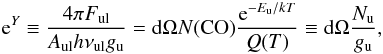 (B.3)
(B.3)
with the column density per level 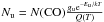 . Thus,
 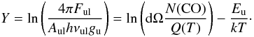 (B.4)We note that the rotation diagram is often given by assuming that Ful = dΩbeamIul, for the solid angle of the telescope beam
  , thus the molecules are equally distributed over the beam. This is however inappropriate for the CO ladder probing a wide range of temperatures and subsequently different emitting regions (Sect. 3.4).
How do opacity effects alter the rotation diagram? Assuming a square line profile of (velocity) width Δv for simplicity and neglecting the background intensity, we obtain for the integrated intensity using Eq. (A.14)), 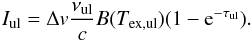 (B.5)For τul ≪ 1,
  , recovering the expression used in Eq. (B.2). For τul > 1,
  , which is always larger than the optically thin expression. Thus, optical depth effects shift points above the optically thin lines in the rotation diagram.
© ESO, 2012
Current usage metrics show cumulative count of Article Views (full-text article views including HTML views, PDF and ePub downloads, according to the available data) and Abstracts Views on Vision4Press platform.
Data correspond to usage on the plateform after 2015. The current usage metrics is available 48-96 hours after online publication and is updated daily on week days.
Initial download of the metrics may take a while.