| Issue |
A&A
Volume 537, January 2012
|
|
|---|---|---|
| Article Number | A59 | |
| Number of page(s) | 11 | |
| Section | Stellar structure and evolution | |
| DOI | https://doi.org/10.1051/0004-6361/201117922 | |
| Published online | 09 January 2012 | |
Online material
Appendix A: Details of spectroscopic observations and their analyses
A.1. Observational equipment
Here we provide more details on the spectra used in this study (see Table 1) and their reduction:
-
1.
Ondřejov spectra: All 439 spectra were obtained in the coudéfocus of the 2.0 m reflector and have a lineardispersion 17.2 Å.mm-1 and a 2–pixel resolution R ~ 12 600 (~11–12 km s-1 per pixel). The first 318 spectra were taken with a Reticon 1872RF detector. Complete reductions of these spectrograms were carried out by Mr. Josef Havelka, Mr. Pavol Habuda and by PH in the program SPEFO. The remaining spectra were secured with an SITe–5800 × 2000 CCD detector. Their initial reductions (bias substraction, flatfielding, extraction of 1D image and wavelength calibration) were done by MŠ with the IRAF program.
-
2.
DAO spectra: all 136 spectra were obtained in the coudé focus of the 1.22 m Dominion Observatory reflector by SY, who carried out initial reductions (bias substraction, flatfielding, extraction of 1D image). The wavelength calibration of the spectra was carried out by JN in SPEFO. The spectra were obtained with the 32121H spectrograph with the IS32R image slicer. The detectors were UBC–1 4096 × 200 CCD for the data prior to May 2005 and SITe–4 4096 × 2048 CCD for the data after May 2005. The spectra have a linear dispersion of 10 Å.mm-1 and 2–pixel resolution R ~ 21 700 (s~7 km s-1 per pixel).
-
3.
OHP spectra: Public ELODIE archive5 of the Haute Provence Observatory (Moultaka et al. 2004) contains 35 echelle spectra obtained at the 1.93 m telescope. They have resolution R ~ 42 000. Initial reductions (bias substraction, flatfielding, extraction of 1D image, and wavelength calibration) was carried out at the OHP. We only extracted and studied the red parts of the spectra.
-
4.
Ritter spectra: All 204 spectra were obtained with a fiber-fed echelle spectrograph at the 1 m telescope of the Ritter Observatory of the University of Toledo. We obtained spectra in form of ASCII table covering only region close to Hα spectra line. The resolution of the spectra is R ~ 26 000. Initial reductions of spectra (bias substraction, flatfielding, extraction of 1D image and wavelength calibration) were carried out at the Ritter Observatory with the IRAF program.
-
5.
Castanet Tolosan and OHP spectra: We downloaded these spectra from the Be Star Spectra database6. All of them were obtained by CB with several different spectrographs7. Only spectra with a resolution comparable to spectra obtained at the rest of observatories were used in the study. Initial reductions (bias substraction, flatfielding, extraction of 1D image, and wavelength calibration) were carried out by CB.
For all individual spectrograms, the zero point of the heliocentric wavelength scale was corrected via the RV measurements of selected unblended telluric lines in SPEFO (see Horn et al. 1996, for details).
Orbital elements obtained using RVs measured on the emission wings of He i 6678 Å line, absorption core of the He i 6678 Å line, and emission wings of the Si II 6347 Å and Si II 6371 Å lines. RJD = HJD–2 400 000.
A.2. Additional RV measurements
We measured RVs on emission wings and absorption core of He i 6678 Å and emission wings of Si II 6347 Å and Si II 6371 Å lines. The program SPEFO was used to the task. The precision of these RV measurements is quite low, since the relative flux in the lines is only several percent greater than in surrounding continuum (see Fig. 2). One could be easily misled during measurements, because measured lines are deformed with continuum fluctuations, and they blend with telluric lines. Despite these complications RVs measured on these lines exhibit long-term variations very similar to the variations that can be seen in Fig. 6. RVs measured on emission wings of He i 6678 Å line, absorption core of He i 6678 Å line, and emission wings of Si II 6347 Å and Si II 6371 Å lines are shown in Fig. A.1.
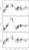 |
Fig. A.1
A time plot of the RVs measured manually in SPEFO. Top panel: the emission wings of the He i 6678 Å line, middle panel: the absorption core of the He i 6678 Å line, bottom panel: the emission wings of Si II 6347 Å and Si II 6371 Å lines. The HEC13 model of the long-term variations is shown by a solid line in each panel. |
| Open with DEXTER | |
The long-term variations were removed with the program HEC13, using the 200 d normals and ϵ = 5 × 10-16. The model of long-term variations derived by HEC13 is shown in Fig. A.1. The residua were searched for periodicity using the HEC27 program. A period near 200 d was detected in all cases, although with a lower significance than the Hα emission RV (see Figs. 7 and 8). The θ statistics periodograms for trial periods from 3000 0 down to 500 are shown in Fig. A.2, where the period P = 2030 is denoted. The θ mininum for this period is not the dominant one only in the case of RV measured on the silicon lines. It is probably due to their low precision and/or incomplete removal of the long-term changes via HEC13.
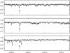 |
Fig. A.2
The θ statistics periodograms. Top panel: the emission wings of He i 6678 Å line, middle panel: the absorption core of He i 6678 Å line, bottom panel: the emission wings of Si II 6347 Å and Si II 6371 Å lines. The period P = 203 |
| Open with DEXTER | |
The circular-orbit solutions were computed for all prewhitened RVs, keeping the orbital period fixed at the value P = 20352. The corresponding orbital elements are in Table A.1.
Data smoothing with different γ velocities derived with the SPEL program was tested as well. It led to none or a slight (lower than 5%) improvement in rms for the Keplerian fit.
In passing, we wish to mention that the Gaussian fits of the Hα line also provided individual RVs of this line. Not surprisingly, a Keplerian fit of these RVs resulted in a semiamplitude lower than was obtained for the directly measured RVs and for some 40% greater rms than that for our preferred solution 5.
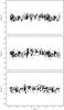 |
Fig. A.3
Phase diagrams of RVs prewithened with HEC13. Top panel: the emission wings of the He i 6678 Å line, middle panel: the absorption core of the He i 6678 Å line, bottom panel: the emission wings of the Si II 6347 Å and Si II 6371 Å lines. The period P = 203 |
| Open with DEXTER | |
A.3. Comparison
PH and JN measured RVs independently on spectra obtained with Reticon detector at Ondřejov observatory. Comparison of their results is shown in Fig. A.4. Dependency was fitted with linear function y = a.x. The resulting parameters are emission wings of Hα line a = 1.024 ± 0.006, emission wings of He i 6678 Å line a = 1.038 ± 0.024, absorption core of He i 6678 Å line a = 1.022 ± 0.008. Differences between the measurements of both authors are quite high for He i 6678 Å line emission wings measurements. It is probably because wings of the line are affected by the background noise and because the red peak of the He i 6678 Å line is very low at some point in the V / R cycle.
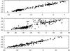 |
Fig. A.4
RVs measured by JN plotted vs. RVs measured by PH on spectra obtained at Ondřejov Observatory with Reticon detector. Top panel: emission wings of Hα line, middle panel: emission wings of He i 6678 Å line, bottom panel: absorption core of He i 6678 Å line. |
| Open with DEXTER | |
© ESO, 2012
Current usage metrics show cumulative count of Article Views (full-text article views including HTML views, PDF and ePub downloads, according to the available data) and Abstracts Views on Vision4Press platform.
Data correspond to usage on the plateform after 2015. The current usage metrics is available 48-96 hours after online publication and is updated daily on week days.
Initial download of the metrics may take a while.