| Issue |
A&A
Volume 535, November 2011
|
|
|---|---|---|
| Article Number | A92 | |
| Number of page(s) | 11 | |
| Section | The Sun | |
| DOI | https://doi.org/10.1051/0004-6361/201117885 | |
| Published online | 17 November 2011 | |
Online material
Appendix A: solution of the focused diffusion equation for α ≠ 2
Equation (7) can be solved by performing a Laplace transformation on the equation and transferring the corresponding homogeneous second-order differential equation into a modified Bessel differential equation. A particular solution to the inhomogeneous equation can be found with the variation-of-constants method, and the inverse Laplace transformation finally reveals the desired solution.
A.1. Laplace transformation
Performing a Laplace transformation in the time coordinate to the diffusion Eq. (7) yields, with the boundary condition limT → 0F(T) = 0 and after some simplifications, 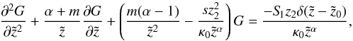 (A.1)where
 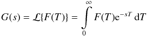 (A.2)is the Laplace transform of F(T).
A.2. Homogeneous solution for α ≠ 2
With the substitution 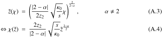 and
and 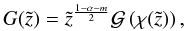 (A.5)Eq. (A.1) transforms into
 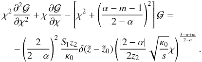 (A.6)The corresponding homogeneous equation
 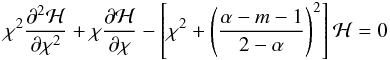 (A.7)is the well known modified Bessel differential equation with the two linearly independent solutions:
 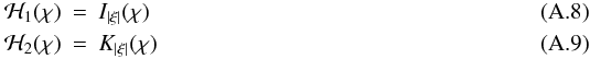 where
where 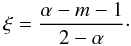 (A.10)Accordingly,
 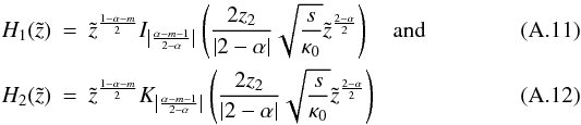 form a fundamental system for the homogeneous differential equation corresponding to Eq. (A.1):
 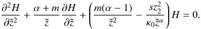 (A.13)
A.3. Particular solution for α ≠ 2
A particular solution to the inhomogeneous Eq. (A.1) can be found with the variation-of-constants method. According to this method two functions  and
and  exist, that solve the linear equation system:
 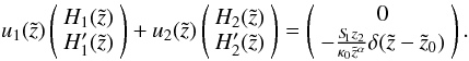 (A.14)The solutions are
 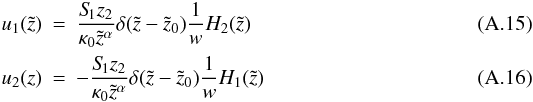 where w is the Wronskian
 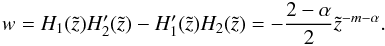 (A.17)A particular solution is given by
  (A.18)where
  and
and  are integrals of and .
For α < 2 we choose 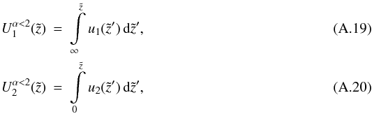 and the particular solution reads as
 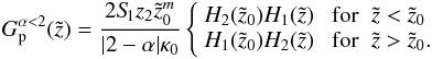 (A.21)For α > 2 we choose
 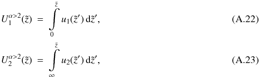 and the particular solution reads as
 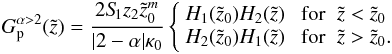 (A.24)
A.4. Inverse Laplace transformation
The general solution to the differential Eq. (A.1) is the superposition of the homogeneous solutions  and
and  , plus the particular solution
  :
:  (A.25)The constants c1 and c2 can be determined by the chosen spatial boundary conditions. We cannot find an inverse Laplace transformation for the exponentially growing function
  and choose c1(s) = 0. Using the relation (5.16.42) from Erdelyi (1954) for a > 0,
 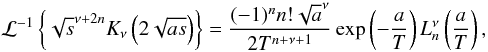 (A.26)where
  denotes the generalized Laguerre polynomials, we find
 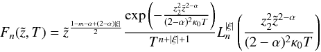 (A.27)as homogeneous solutions to the differential Eq. (7). We now perform an inverse Laplace transformation to the particular solution
  . Utilizing the relation 5.16.56 from Erdelyi (1954),
 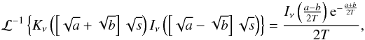 where ℜ(a) > 0 and ℜ(b) > 0 has to be fulfilled, we receive
 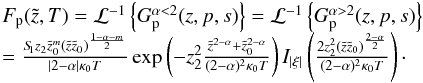 (A.28)Every superposition
 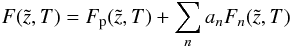 (A.29)is a solution of Eq. (7). A solution fulfilling the boundary conditions (12) − (14) and (16) for
  is given by
  . As an aside, we note that the particular solution is an infinite sum of the homogeneous solutions (A.27):
 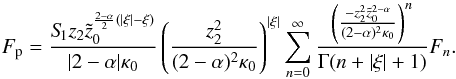 (A.30)
Appendix B: solution of the focused diffusion equation for α = 2
For α = 2 the Laplace transformed focused diffusion Eq. (A.1) reads as 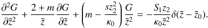 (B.1)With the ansatz
  (B.2)we find the corresponding homogeneous solutions:
 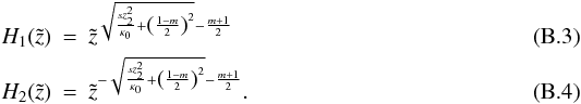 Again, a particular solution can be found utilizing the variation-of-constants method:
 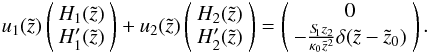 (B.5)The solutions for this linear system of equations are
 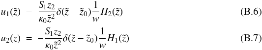 with the Wronskian:
 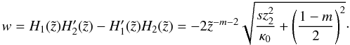 (B.8)A particular solution for Eq. (B.1) is therefore given by
  (B.9)where and are integrals of and .
If we choose 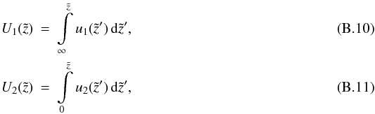 the particular solution reads as
 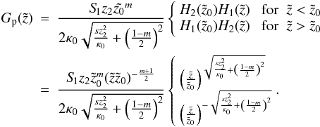 (B.12)Using the relation (5.6.6) from Erdelyi (1954)
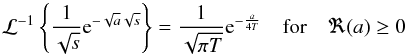 (B.13)we find
 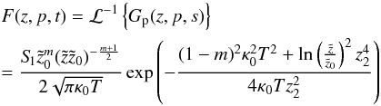 (B.14)as a solution for the time-dependent focused diffusion equation for α = 2.
© ESO, 2011
Current usage metrics show cumulative count of Article Views (full-text article views including HTML views, PDF and ePub downloads, according to the available data) and Abstracts Views on Vision4Press platform.
Data correspond to usage on the plateform after 2015. The current usage metrics is available 48-96 hours after online publication and is updated daily on week days.
Initial download of the metrics may take a while.