| Issue |
A&A
Volume 535, November 2011
|
|
|---|---|---|
| Article Number | A92 | |
| Number of page(s) | 11 | |
| Section | The Sun | |
| DOI | https://doi.org/10.1051/0004-6361/201117885 | |
| Published online | 17 November 2011 | |
A diffusive description of the focused transport of solar energetic particles
Intensity- and anisotropy-time profiles as a powerful diagnostic tool for interplanetary particle transport conditions⋆
1 Institut für Theoretische Physik, Lehrstuhl IV: Weltraum- und Astrophysik, Ruhr-Universität Bochum, 44780 Bochum, Germany
e-mail: sa@tp4.rub.de
2 Space Sciences Laboratory, University of California, Berkeley, CA 94720-7450, USA
3 Departament d’Astronomia i Meteorologia, Institut de Ciències del Cosmos (ICC), Universitat de Barcelona, Spain
4 Physics Department, University of California, Berkeley, CA 94720-7300, USA
5 School of Space Research, Kyung Hee University, Yongin, Gyeonggi, Korea
Received: 15 August 2011
Accepted: 9 September 2011
The transport of solar energetic charged particles along the interplanetary magnetic field in the ecliptic plane of the sun can be described roughly by a one-dimensional diffusion equation. Large-scale spatial variations of the guide magnetic field can be taken into account by adding an additional term to the diffusion equation that includes the effect of adiabatic focusing. We solve this equation analytically by assuming a point-like particle injection in time and space and a spatial power-law dependence for the focusing length and the spatial diffusion coefficient. We infer the intensity- and anisotropy-time profiles of solar energetic particles from this solution. Through these the influence of different assumptions for the diffusion parameters can be seen in a mathematically closed form. The comparison of calculated and measured intensity- and anisotropy-time profiles, which are a powerful diagnostic tool for interplanetary particle transport, gives information about the large-scale spatial dependence of the focusing length and the diffusion coefficient. For an exceptionally large solar energetic particle event, which did occur on 2001 April 15, we fit the 27 − 512 keV electron intensities and anisotropies observed by the Wind spacecraft using the theoretically derived profiles. We find a linear spatial dependence of the mean free path along the guiding magnetic field. We also find the mean free path to be energy independent, which supports the theory of “velocity-dependent diffusion”. This means that the intensity profiles for the discussed energies exhibit the same shape if they are plotted against the traveled distance and not against the time. In this case the profiles differ only in their maximum values and we can determine the energy spectra of the solar flare electrons out of the scaling factor we need to fit the data. The derived spectra exhibits a power-law dependence ∝  in an energy range from ~ 50 keV to ~ 500 keV.
Key words: solar wind / Sun: magnetic topology / scattering / diffusion / stars: flare
Appendices are available in electronic form at http://www.aanda.org
© ESO, 2011
1. Introduction
Modeling the transport of solar energetic particles has been in the focus of interest for several years. Most models assume a large-scale structure of a guide magnetic field, B0, with superposed small irregularities, δB. The energetic charged particles move along this guide magnetic field B0 performing a gyration motion around the large-scale magnetic field lines. The small superposed irregularities interact with the gyrating particles in such a way that the first adiabatic invariant (the magnetic moment) is not conserved, leading to a scattering of the pitch angle, θ (angle between the velocity vector v of the particles and B0). As can be seen, for example, in the first chapter of Shalchi (2009), this pitch-angle scattering leads to a diffusive motion of the particle’s guiding centers along B0.
Whereas early transport models (Meyer et al. 1956) are based on a simple, empirically found, one-dimensional diffusion equation in space, later and more complete models describe the evolution of the phase-space density in the test-particle approach by a Fokker-Planck type transport equation that can be derived from the equation of continuity in phase space. This equation may take additional effects into account that arise, for example, from the spatial variation in the guiding magnetic field. A lot of work has been done in simulating this transport by numerically solving Fokker-Planck equations that include different effects, such as adiabatic focusing, adiabatic cooling or perpendicular diffusion, assuming different types of magnetic turbulence that lead to different shapes of the diffusion coefficients (for review see Dröge & Kartavykh 2009; Dröge et al. 2010; Dröge 2003; Agueda et al. 2008; Qin et al. 2004; Ruffolo 1995).
For an analytical treatment, the Fokker-Planck type transport equation has to be simplified. This is normally done by assuming a near isotropic distribution function and applying a diffusion approximation to the transport equation. The result is again a diffusion equation, known from the early models describing cosmic ray transport, which can be solved analytically in many cases. The advantage of this circuitous derivation of the diffusion equation is that some of the previously described transport effects can be accounted for in the diffusion regime. In this work we concentrate on the effect of adiabatic focusing.
Adiabatic focusing arises in the case of a slowly varying guide magnetic field B0. “Slowly” means that the typical length scale that characterizes the change in B0 is large compared to the spatial dimension of the particles’ gyration motion. In this case it can be assumed that B0 is constant for a single gyration, and the first adiabatic invariant is conserved. For a particle moving in a diverging magnetic field, this conservation of the magnetic moment leads to an energy transfer from the perpendicular to the parallel motion, resulting in a decreasing pitch angle, which justifies the name “adiabatic focusing”. For a particle moving in a converging magnetic field, the energy transfer is vice versa. The total energy is conserved in both scenarios.
In Sect. 2 of this paper we present an analytical solution to the one-dimensional focused diffusion equation, where we assume a spatial power-law dependence for the spatial diffusion coefficient κ and the background magnetic field B0. In Sects. 3 and 4 we derive the corresponding intensity- and anisotropy-time profiles. We compare the analytical results with in-situ measurements of solar electrons in Sect. 5. We summarize this work in Sect. 6.
2. The focused diffusion equation
The time-dependent one-dimensional diffusion equation including the effect of adiabatic focusing reads as (Earl 1976)1![\begin{equation} \label{eq:fde} \frac{\partial F}{\partial t}- \frac{\partial}{\partial z}\left( \kappa \left[\frac{\partial F}{\partial z} - \frac{F}{L}\right] \right) = S(z,p,t), \end{equation}](/articles/aa/full_html/2011/11/aa17885-11/aa17885-11-eq13.png) (1)where
(1)where  (2)denotes the isotropic part of the assumed gyrotropic phase-space density f(z,p,μ,t), μ is the pitch-angle cosine, L is the focusing length,
  (3)and S(z,p,t) represents the source distribution.
Assuming a point-like injection source in time and space  (4)and a spatial power-law dependence for the guide magnetic field B0(z) and the diffusion coefficient κ(z),
  the diffusion Eq. (1) reads as2
![\begin{equation} \label{eq:fde2} \frac{\partial F}{\partial T}- \frac{1}{z_2^2}\frac{\partial}{\partial \tilde{z}}\left(\kappa_0 \tilde{z}^{\alpha} \left[\frac{\partial F}{\partial \tilde{z}} + \frac{m}{\tilde{z}} F\right]\right) = \frac{S_{\hspace{-0.07 cm}1}(p)}{z_2} \delta(\tilde{z}-\tilde{z}_0) \delta(T) \end{equation}](/articles/aa/full_html/2011/11/aa17885-11/aa17885-11-eq24.png) (7)with the abbreviations,
(7)with the abbreviations,  (8)Here z1 ≥ 0 denotes a translation to avoid an infinitely large magnetic field at the Sun (z = 0) for m < 0, and z2 > 0 denotes a scaling length to introduce dimensionless quantities.
Furthermore, we defined the particles mean free path  (9)with the particles velocity v, according to the mean free path of a three-dimensional self-diffusion process3.
For the boundary conditions mentioned below, Eq. (7) can be solved analytically. The solution for α ≠ 2 is given by 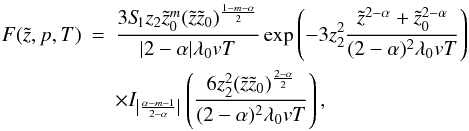 (10)where I|ξ| represents the modified Bessel function of the first kind and
  the mean free path at z = z2 − z1 (see Appendix A for details). In the case of a linear spatial dependence of the mean free path λ (α = 1) and a positive focusing length L (m < 0), this solution agrees with the one presented in Kocharov et al. (1996) for z1 = 0. A similar solution in a different context can also be found in Toptygin (1985).
Though the presented solution (10) solves Eq. (7) for α ∈ ℝ\{2} and m ∈ ℝ, we reduce our analysis to the case  (11)where (10) fulfills the following physically meaningfull initial and boundary conditions:
i): F(t = t0) vanishes everywhere except at the source:  (12)
(12)
ii): the particle flux density, ![\begin{equation} J(z,p,T)= -\kappa \left[\frac{\partial F}{\partial z} - \frac{F}{L}\right], \end{equation}](/articles/aa/full_html/2011/11/aa17885-11/aa17885-11-eq46.png) (13)vanishes for z → ∞,
(13)vanishes for z → ∞,  (14)and is small for z → 0,
  (15)for z1 ≪ z2 the boundary condition (15) can be approximated by
  (16)
(16)
In the case of a constant magnetic field and a constant diffusion coefficient (m = α = 0) there is no need for the translation z1, and we can set z1 = 0. In this case Eq. (10) simplifies to  (17)in agreement with the solution of the focused diffusion Eq. (1) for constant κ = κ0, and L that fulfills the boundary conditions (12, 14) and limz → 0F(z) = 0
  (18)in the limiting case L → ∞.
3. Intensity profiles
The omnidirectional intensity  is connected to the isotropic phase-space density by the simple relation (Rossi & Olbert 1970):
  (19)By inserting Eq. (10) into (19) we get an analytic expression for the omnidirectional intensity depending on the time T, the position z, the spatial diffusion coefficient
  , and the power-law dependence of the magnetic field m.
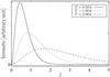 |
Fig. 1 Sketch of the temporal evolution of the spatial intensity distribution of solar energetic particles released instantaneously at T = 0 for α = 1 and m = −2. |
Figure 1 shows the temporal evolution of the spatial intensity distribution. Energetic particles are released at the Sun instantaneously at T = 0, represented by a delta-function δ(T). Due to pitch-angle scattering, this delta function develops into a Gaussian with a time-dependent FWHM. The effect of adiabatic focusing and the assumed boundary conditions lead to a modification of this Gaussian by the Bessel function Iξ, which results in an a outward movement of the bulk of the particles. This seems to be a convincing solution, but only to a certain degree. It cannot be avoided that a (Markovian) diffusive description of particle propagation violates the basic causality law of special relativity. For times T > 0, the asymptotic behavior of the intensity profile  includes a nonvanishing probability of particles travelling faster than the speed of light. A non-Markovian generalization of this diffusion model, as described in Dunkel et al. (2007), could avoid this violation.
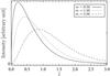 |
Fig. 2 Sketch of the spatial dependence of the intensity distribution on the magnetic field structure (Eq. (5)) at a given time T = 1 h for α = 1. |
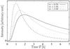 |
Fig. 3 Sketch of the temporal dependence of the intensity distribution on the magnetic field structure (Eq. (5)) at a given position |

Figures 2 and 3 sketch the influence of the magnetic field spatial variation (Eq. (5)) on the intensity-time and intensity-space profile. It can be seen that particles in a diverging magnetic field with m = −2 propagate faster in the parallel direction than those in a field with m = −1 and with m = −0.5. The physical explanation for this is the effect of adiabatic focusing that transfers energy from gyration to translation along the field lines in a diverging field and that has a stronger effect for m = −2.
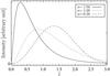 |
Fig. 4 Sketch of the spatial dependence of the intensity distribution on the spatial power-law dependence of the diffusion coefficient at a given time T = 1 h for m = −2. |
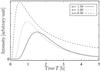 |
Fig. 5 Sketch of the temporal dependence of the intensity distribution on the spatial power-law dependence of the diffusion coefficient at a given position |
Figures 4 and 5 illustrate the dependence of the omnidirectional intensity on spatial variations of the diffusion coefficient (or mean free path). For better comprehension of the displayed curve progressions Fig. 6 shows the mean free path, λ, as a function of the distance  . Combining Figs. 4 and 6, we see that a short mean free path results in a slow and a long mean free path in a fast diffusion process. This means that particles spend more time in an area with a short mean free path, as expected. It can also be seen that the area under the curves in Fig. 4 is the same. This is a consequence of our postulated boundary conditions where we required a conservation of the number of particles between
  and
and  . Figure 5 exhibits a lower density of particles moving with a higher bulk velocity due to a larger mean free path.
4. Anisotropy-time profiles
Beside the omnidirectional intensity, which carries information about the particle flux averaged over the solid angle, the diffusive description also allows for directional information of the particle propagation. This information can be expressed in terms for the anisotropy of the particle distribution. For a gyrotropic phase-space density f(z,p,μ,T), the first-order anisotropy A(z,p,T) is defined as 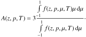 (20)Because f(z,p,μ,T) ≥ 0 is proportional to the probability distribution, the anisotropy A represents three times the expectation value of the pitch-angle cosine μ and is limited by
 If we express f(z,p,μ,T) in terms of the isotropic and anisotropic part, F(z,p,T) and g(z,p,μ,T), of the phase-space density
  (21)we find
  (22)According to the diffusion approximation presented in Schlickeiser et al. (2007) and Schlickeiser & Shalchi (2008), the anisotropic part, g(z,p,μ,T),
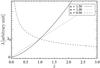 |
Fig. 6 Sketch of the spatial dependence of the mean free path λ for three different powers. |
can be expressed in the weak focusing limit and for negligible perpendicular diffusion as ![\begin{eqnarray} \label{eq:Ge2} &&g(z,p,\mu,T)=\overbrace{\left[ \int\limits_{-1}^{1} \frac{(1-\mu) D_{\mu p}(\mu)}{D_{\mu \mu}(\mu)} \mathrm{d} \mu - 2 \int\limits_{-1}^{\mu}\frac{D_{\mu p}(x)}{D_{\mu \mu}(x)}\mathrm{d} x \right] \frac{1}{2}\frac{\partial F}{\partial p}}^{=g_{\rm cg}} \nonumber\\ &&+\underbrace{\left[ \int\limits_{-1}^{1} \frac{(1-\mu)(1-\mu^2)}{D_{\mu \mu}(\mu)} \mathrm{d} \mu -2 \int\limits_{-1}^{\mu} \frac{(1-x^2)}{D_{\mu \mu}(x)}\mathrm{d}x \right]\frac{v}{4}\left(\frac{\partial F}{\partial z}-\frac{F}{L}\right)}_{= g_{\rm s}}\cdot \end{eqnarray}](/articles/aa/full_html/2011/11/aa17885-11/aa17885-11-eq91.png) (23)Evidently, g(z,p,μ,T) consists of a Compton-Getting part, gcg, and a streaming part, gs. Consequently, we split our anisotropy into two parts,
(23)Evidently, g(z,p,μ,T) consists of a Compton-Getting part, gcg, and a streaming part, gs. Consequently, we split our anisotropy into two parts,  (24)and by inserting Eq. (23) into (22) we find
 ![\begin{eqnarray} A_{\rm s}(z,p,T)&=& - 3 \frac{\kappa}{v} \left[ \frac{\partial \ln(F)}{\partial z}-\frac{1}{L} \right]=-\lambda \left[ \frac{\partial \ln(F B_0)}{\partial z}\right]\label{eq:As}\\ A_{\rm cg}(z,p,T)&=& - \frac{3a_{11}}{4} \frac{\partial\ln(F)}{\partial p} \label{eq:Acg} \end{eqnarray}](/articles/aa/full_html/2011/11/aa17885-11/aa17885-11-eq95.png) where we identified the spatial diffusion coefficient,
where we identified the spatial diffusion coefficient,  (27)and introduced the rate of adiabatic deceleration:
  (28)It is important to notice that the diffusion approximation only holds if the phase-space density f(z,p,μ,T) is close to the isotropic equilibrium distribution F(z,p,T), which means | g(z,p,μ,T) | ≪ F(z,p,T). If the anisotropic part exceeds the isotropic one, Eq. (23) no longer accounts for the anisotropic part. A violation of this requirement gives rise to negative values of the phase-space density (21) and causes absolute values of the anisotropy to be higher than three. The anisotropy is therefore an indicator of the validity of the diffusive particle transport description.
As shown in Schlickeiser et al. (2009), the Compton-Getting anisotropy (Eq. (26)) is small compared to the streaming anisotropy (Eq. (25)) for solar energetic particles observed at 1 AU. Therefore it will be neglected.
We use Eqs. (25) and (10) to calculate the anisotropy-time profile of solar energetic particles with the assumptions of a spatial power-law dependence for the magnetic field B0(z) and the diffusion coefficient κ(z) and find for  :
: ![\begin{equation} A_{\rm s}= \frac{3 \tilde{z} z_2 \left[1-\left({\frac{\tilde{z}_0}{\tilde{z}}}\right)^{\frac{2-\alpha}{2}}\frac{ I_{\xi+1} \left(\frac{2 {z_2}^2 (\tilde{z} \tilde{z}_0)^{\frac{2-\alpha}{2}}}{(2-\alpha)^2 \kappa_0 T}\right)}{ I_{\xi} \left(\frac{2 {z_2}^2 (\tilde{z} \tilde{z}_0)^{\frac{2-\alpha}{2}}}{(2-\alpha)^2 \kappa_0 T}\right)}\right]}{(2-\alpha)vT}\cdot\label{eq:An} \end{equation}](/articles/aa/full_html/2011/11/aa17885-11/aa17885-11-eq101.png) (29)Under typical magnetic field and solar wind conditions, this formal expression for the anisotropy can be simplified in most cases for solar energetic particles observed at z ≈ 1.2 AU. For a magnetic field close to the nominal Parker spiral with m = −2 and for a particle injection in the corona at three solar radii z0 = 0.014 AU with a typical magnetic field strength of B0(z = z0) = 30 μT and a particle detection close to the Earth with a magnetic field strength of B0(z = 1.2 AU) = 5 nT, we choose the scaling length z2 = 1 AU and have to set the translation to z1 = 0.0015 AU. This implies for the observed anisotropy-time profile at z = 1.2 AU:
(29)Under typical magnetic field and solar wind conditions, this formal expression for the anisotropy can be simplified in most cases for solar energetic particles observed at z ≈ 1.2 AU. For a magnetic field close to the nominal Parker spiral with m = −2 and for a particle injection in the corona at three solar radii z0 = 0.014 AU with a typical magnetic field strength of B0(z = z0) = 30 μT and a particle detection close to the Earth with a magnetic field strength of B0(z = 1.2 AU) = 5 nT, we choose the scaling length z2 = 1 AU and have to set the translation to z1 = 0.0015 AU. This implies for the observed anisotropy-time profile at z = 1.2 AU:  . Keeping this relation in mind we take a look at the monotonically increasing function
  (30)with
  and conclude that the second summand in Eq. (29) is small compared to the first if α is small enough compared to 2. In this case the anisotropy simplifies to
  (33)Figure 7 shows a sketch of the exact streaming anisotropy (Eq. (29)) in comparison with the approximated anisotropy (Eq. (33)) for three different values of α. The sketch confirms that the approximation holds if α is small enough compared to 2. For α = −0.5 and α = 1.0, there is only a negligible deviation, but there is a significant deviation for α = 1.5. For typical solar wind conditions and a particle observation at z ≈ 1.2 AU, it can roughly be said that the approximation holds for α ≤ 1. In this case the anisotropy is independent of the global magnetic field structure and the absolute value of the mean free path represented by m and λ0. There is also only a weak dependence for α > 1. On the other hand, Fig. 7 proves that the anisotropy is sensitive to the spatial variation of the diffusion coefficient κ.
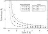 |
Fig. 7 Sketch of the anisotropy-time profile (Eq. (29)) in comparison with the approximation (Eq. (33)) for three different values for α. |
It should be mentioned that the anisotropy tends to infinity for t → t0, in contrast to definition (22) that implies a maximum value of three for the anisotropy. This erratic behavior is a consequence of the violation of the causality law of special relativity discussed in Sect. 3 and the limited scope for applying of the diffusion approximation. The initial particle flux that violates the causality law and reaches the position of detection just after injection is highly anisotropic. The required assumption |g(z,p,μ,T)| ≪ F(z,p,T) of the diffusion approximation is not fulfilled and, as discussed before, anisotropy values over three arise. For later times and lower anisotropy values, the accuracy of the diffusion approximation increases and the anisotropy values become more realistic.
5. Comparison with measured data
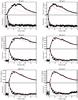 |
Fig. 8 Anisotropy- and intensity-time profiles for 40 − 512 keV electrons measured with the Wind/3DP instrument in comparison with the theoretically derived profile (19) with the parametervalues listed in Table 1. |
The expressions derived in the previous sections for the evolution of the intensity (Eqs. (10) and (19)) and the anisotropy (Eq. (22)) can be compared with in situ measurements during solar energetic electron events. We use electron intensities observed by the three-dimensional plasma and energetic particle (3DP) experiment onboard the Wind spacecraft (Lin et al. 1995). The semi-conductor detector telescopes (SST) of Wind/3DP measure electrons in the energy range 27−512 keV with a full 4π angular coverage in one spacecraft spin period. The pitch-angle distributions provided by SST have a 22.5° resolution and allow the intensity- and anisotropy-time profiles to be calculated for a given event. An exceptionally large solar particle event occurred on 2001 April 15 in association with an X14.4 solar flare located at S20 W85, a type III radio burst and a coronal mass ejection. To reduce the very large number of free parameters in Eqs. (10) and (22) we assume a particle injection at approximately three solar radii (z0 = 0.014 AU) and a distance of z = 1.2 AU along the Archimedean spiral from the Sun to the spacecraft. Furthermore, we assume a magnetic field strength of B0(z = 0) = 30 μT at the Sun.
The MFI instrument onboard the Wind spacecraft measured an interplanetary magnetic field strength close to the Earth of approximately B0(z = 1.2 AU) = 3 nT. We choose the scaling length z2 = 1 AU and use Eq. (5) to determine the translation z1. We can now vary the free parameters α, m, and t0 to find good agreement between the theoretical and the measured profiles. We always determine the source function S1(p) through normalization of our theoretical intensity profile on the measured maximum value for 108 keV,180 keV,306 keV, and 512 keV. For 27 keV,40 keV, and 66 keV electrons we use a different value than the maximum value for the normalization. The reason for this choice is the contamination of this profiles with electrons that gained their energy by a different effect than the initial particle injection. This will become more obvious later in this section.
For the set of parameters displayed in Table 1, we plotted the intensity- and anisotropy-time profiles for six different energies in comparison with the measured profiles.
Set of parameters that provides a good fit to the data for different energies.
As can be seen in Fig. 8 we get a very good fit for electrons with energies of 108 keV and more. For lower energies the intensity fit gets worse. The quality of the anisotropy fit is roughly the same for all six energies. The profiles that are measured in the lowest energy channel ( ≈ 27 keV) reveal poor agreement with the theory and are not shown here. A possible explanation for this growing deviation between measurement and theory for lower electron energies is that particles with lower energies are injected over a longer period of time, which broadens the intensity profile. In addition their injection might be less eruptive, which could explain the slower rise and decay of the measured profile. In this case the assumption of an eruptive injection described by the delta function δ(t − t0) no longer holds.
It is remarkable how well this simplified theory agrees with results of much more detailed computer simulations for this event. Bieber et al. (2004) conclude that the onset of particle injection onto the Sun-Earth field line was at 13:42 UT ± 1 min, and Agueda et al. (2009) conclude that the electron injection started at 13:48 UT at 80 keV. These two previous results are in accordance with our injection time at 13:45 UT. Dröge (2005) modeled the event by assuming a spatially constant radial mean free path for 511 keV electrons and concludes that λr = 0.14 AU (λ∥ = 0.24 AU at Earth). Similarly, Agueda et al. (2009) estimate the radial mean free path of the 62 − 312 keV electrons is 0.08 AU (λ∥ = 0.17 AU at Earth). At the distance of the Earth these agree with our result:  (34)The obtained linear dependence between
  and the parallel mean free path mainly arises from fitting the anisotropy-time profiles. As already said, the anisotropy depends weakly on the power-law dependence of the magnetic field and the value of the mean free path, λ0, for the given boundary conditions. At a given position z the slope of the anisotropy-time profile is only determined by the exponent α of the spatial power-law dependence of the diffusion coefficient and the energy of the particles, represented by v. We can therefore vary the two parameters m and λ0 to fit the intensity-time profiles without changing the anisotropy significantly.
Assuming a constant solar wind speed usw, the model of the Parker spiral (Parker 1958) predicts a radial dependence of the magnetic field strength according to 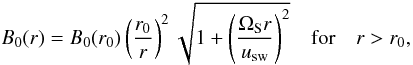 (35)where ΩS is the sidereal solar rotation rate and r0 a radius at which the field is completely frozen into the solar wind. The radial dependence of the pathlength along the Archimedean spiral is given by
 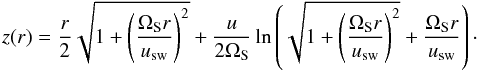 (36)For r < usw/ΩS ≈ 1 AU we approximate z(r) ≈ r and
 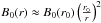 and conclude that m ≈ − 2.
To obtain an acceptable fit we have to deviate from this inverse quadratic dependence of the large scale magnetic field. But the model of the Parker spiral is based on strong simplifications and should be only regarded as an average magnetic field for a longer period of time. For this single event one may also think of particles traveling along a fluxtube with a different spatial dependence of the magnetic field. The deviation may also be caused by the fact that the solar flare location (S20 W85) differs from the footpoint of the Archimedean spiral (S00 W48) assuming the solar wind speed measured at 1 AU of usw ≈ 500 km s-1. Furthermore, we cannot exclude that this different shape of the magnetic field lines is just a local effect in the area where the measurement took place.
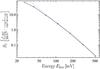 |
Fig. 9 Energy dependence of the injection function S1 (solid black line with crosses) in comparison with a ∝ |
Finally, we take a look at the energy dependence of the source function S1 that we can infer from the normalization factor. In Fig. 9 we plot S1(Ekin) against Ekin and notice that S1 exhibits a clear proportionality to an  power law in the range of the five highest energies. The two lowest energies deviate from this power law and suggest that an exponential decay may also be possible. Considering that the lower energy intensity profiles are strongly contaminated by energetic particles of a different source than the initial injection, one should not overinterpret this deviation. This energy spectrum confirms the result of Heristchi & Amari (1992) that at least some solar flare electron spectra fit well with a power law in energy in a wide energy range.
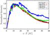 |
Fig. 10 Normalized intensity-distance profiles for four different electron energies. vT represents the distance that the electrons cover after their first detection at the given position. |
Furthermore, our results support the theory of “velocity-dependent diffusion” noted for the first time by Bryant et al. (1964). They have shown that the intensity profiles for various energies reveal the same shape if they are plotted against the traveled distance of the particles (vT, where T is the time after the first particles are detected. In our case, T = t − 14 h ). Figure 10 shows a plot like this for the four highest energy channels of the SST experiment. It can be seen that the variation of all intensity profiles in this energy range is the same and that they only differ in their maximum intensity.
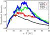 |
Fig. 11 Normalized intensity-distance profiles for the three lowest energies of Wind/3DP in comparison with the 511 keV electrons. |
The sudden deviation that occurs in every profile, with a growing significance for lower energies, is probably caused by an additional injection of mainly lower energetic particles at the Sun. One may also think of an additional acceleration of lower energetic particles at the shock front of the coronal mass ejection that corresponds to this event. Figure 11 demonstrates that this additional disturbance dominates the intensity profiles of the three lowest energies of the SST-F instrument after the rise phase of the intensity profile. This disturbance also explains the poor fit of the intensity-time profiles for 40 keV and 66 keV electrons displayed in Fig. 8 and justifies our normalization to a different value than the measured maximum value for 27 keV,40 keV, and 66 keV electrons.
Encouraged by our results of energy-independent λ0 and α, we propose the concept of “velocity-dependent diffusion” to the anisotropy. Equations (29) and (33) predict that the anisotropy depends only on vT at a given position for constant λ0 and α. Accordingly, we should get the same profile for each energy if we plot the anisotropy against vT. In fact, we discover this feature in the data as can be seen in Fig. 12. This explains our good fits between the measured and the theoretically derived anisotropy for each energy channel with the same set of parameters.
6. Summary and conclusions
We solved the one-dimensional diffusion transport equation of solar energetic particles including the effect of adiabatic focusing for a spatial power-law dependence of the large-scale magnetic field B0 and the diffusion coefficient κ. As boundary conditions we assumed a vanishing phase-space density for t → t0 and a vanishing particle flux at z ≈ 0 and z = ∞. We used our solution to deduce intensity and anisotropy-time profiles that provide a powerful diagnostic tool for estimating the interplanetary particle transport conditions.
We discussed the scope of applying our approximation and pointed out that the anisotropy value is one indicator for the accuracy of our theory. The diffusion approximation does not hold for high anisotropy values. In addition we have to accept that every Markovian diffusion process violates the causality law of special relativity. For a solar flare event, these two sources of error are only influential for a short period of time after the particle injection.
We compared our theoretically derived profiles to the solar 27−512 keV electron event observed by Wind/3DP on 2001 April 15. We find good agreement for electrons with energies of 180 keV up to 512 keV. The agreement diminishes for electrons with energies below 180 keV, for which an additional acceleration mechanism seems plausible. Beside this, the area of validity is restricted to particles with velocities that are much faster than the solar wind. By fitting the data we find an energy-independent mean free path of approximately λ(z) = 0.17z and a spatial dependence of the magnetic field strength given by
 In the case of an Archimedean spiral, we would expect an exponent of m = −2. We listed several possible explanations for this deviation.
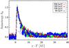 |
Fig. 12 Anisotropy-distance profiles for four different electron energies. |
By fitting the data with our theory, we determined the source spectrum of the solar flare electrons and found a ∝ power law for energies Ekin ∈ ~ [50, 500] keV. Finally, we confirmed that, in the given energy range, the shape of all intensity profiles may be reduced to one characteristic profile by plotting the data against the “traveled distance since the first particle detection” instead of the time. We proved that this feature of a pure vT dependence is reflected by the anisotropy, too, and is predicted by our theory in the case of energy-independent λ0, m, and α.
We conclude that the transport of solar energetic particles is, at least for some events, a spatial diffusion process that is basically described well by a modified diffusion equation (with a spatial and velocity dependent diffusion coefficient κ ∝ vz) that takes the large-scale magnetic field structure into account. Momentum diffusion can be neglected for these timescales.
Online material
Appendix A: solution of the focused diffusion equation for α ≠ 2
Equation (7) can be solved by performing a Laplace transformation on the equation and transferring the corresponding homogeneous second-order differential equation into a modified Bessel differential equation. A particular solution to the inhomogeneous equation can be found with the variation-of-constants method, and the inverse Laplace transformation finally reveals the desired solution.
A.1. Laplace transformation
Performing a Laplace transformation in the time coordinate to the diffusion Eq. (7) yields, with the boundary condition limT → 0F(T) = 0 and after some simplifications, 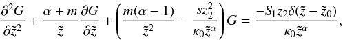 (A.1)where
 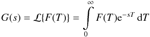 (A.2)is the Laplace transform of F(T).
A.2. Homogeneous solution for α ≠ 2
With the substitution 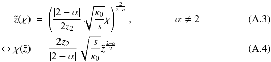 and
and  (A.5)Eq. (A.1) transforms into
 ![\appendix \setcounter{section}{1} \begin{eqnarray} \label{eq:fdelt1} &&\chi^2 \frac{\partial^2 \mathcal{G}}{\partial \chi^2}+\chi \frac{\partial \mathcal{G}}{\partial \chi}- \left[\chi^2+\left(\frac{\alpha-m-1}{2-\alpha}\right)^2 \right] \mathcal{G}= \nonumber\\ && \hspace*{4mm}-\left(\frac{2}{2-\alpha}\right)^2 \frac{S_{\hspace{-0.07 cm}1} z_2}{\kappa_0} \delta(\tilde{z}-\tilde{z}_0) \left(\frac{|2-\alpha|}{2 z_2} \sqrt{\frac{\kappa_0}{s}} \chi \right)^{\frac{3-\alpha+m}{2-\alpha}}. \end{eqnarray}](/articles/aa/full_html/2011/11/aa17885-11/aa17885-11-eq183.png) (A.6)The corresponding homogeneous equation
(A.6)The corresponding homogeneous equation ![\appendix \setcounter{section}{1} \begin{equation} \chi^2 \frac{\partial^2 \mathcal{H}}{\partial \chi^2}+\chi \frac{\partial \mathcal{H}}{\partial \chi}- \left[\chi^2+\left(\frac{\alpha-m-1}{2-\alpha}\right)^2 \right] \mathcal{H} = 0 \end{equation}](/articles/aa/full_html/2011/11/aa17885-11/aa17885-11-eq184.png) (A.7)is the well known modified Bessel differential equation with the two linearly independent solutions:
(A.7)is the well known modified Bessel differential equation with the two linearly independent solutions:  where
where  (A.10)Accordingly,
 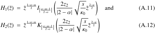 form a fundamental system for the homogeneous differential equation corresponding to Eq. (A.1):
 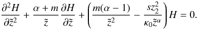 (A.13)
A.3. Particular solution for α ≠ 2
A particular solution to the inhomogeneous Eq. (A.1) can be found with the variation-of-constants method. According to this method two functions  and
and  exist, that solve the linear equation system:
 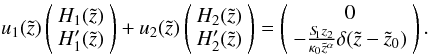 (A.14)The solutions are
 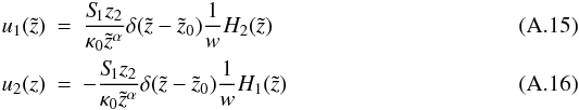 where w is the Wronskian
  (A.17)A particular solution is given by
  (A.18)where
  and
and  are integrals of and .
For α < 2 we choose  and the particular solution reads as
  (A.21)For α > 2 we choose
  and the particular solution reads as
  (A.24)
A.4. Inverse Laplace transformation
The general solution to the differential Eq. (A.1) is the superposition of the homogeneous solutions  and
and  , plus the particular solution
  :
:  (A.25)The constants c1 and c2 can be determined by the chosen spatial boundary conditions. We cannot find an inverse Laplace transformation for the exponentially growing function
  and choose c1(s) = 0. Using the relation (5.16.42) from Erdelyi (1954) for a > 0,
 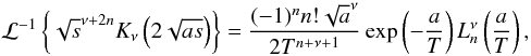 (A.26)where
  denotes the generalized Laguerre polynomials, we find
 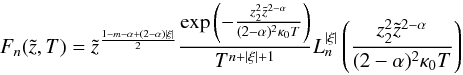 (A.27)as homogeneous solutions to the differential Eq. (7). We now perform an inverse Laplace transformation to the particular solution
  . Utilizing the relation 5.16.56 from Erdelyi (1954),
 ![\appendix \setcounter{section}{1} \begin{displaymath} \mathcal{L}^{-1}\left\{K_\nu\left(\left[\sqrt{a}+ \sqrt {b}\right] \sqrt{s} \right)I_\nu \left(\left[\sqrt{a} - \sqrt{b}\right]\sqrt{s} \right)\right\}=\frac{I_\nu \left(\frac{a-b}{2T} \right)\mathrm{e}^{-\frac{a+b}{2T}}}{2T}, \end{displaymath}](/articles/aa/full_html/2011/11/aa17885-11/aa17885-11-eq217.png) where ℜ(a) > 0 and ℜ(b) > 0 has to be fulfilled, we receive
where ℜ(a) > 0 and ℜ(b) > 0 has to be fulfilled, we receive 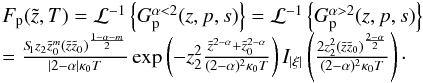 (A.28)Every superposition
 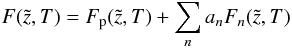 (A.29)is a solution of Eq. (7). A solution fulfilling the boundary conditions (12) − (14) and (16) for
  is given by
  . As an aside, we note that the particular solution is an infinite sum of the homogeneous solutions (A.27):
 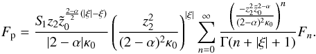 (A.30)
Appendix B: solution of the focused diffusion equation for α = 2
For α = 2 the Laplace transformed focused diffusion Eq. (A.1) reads as 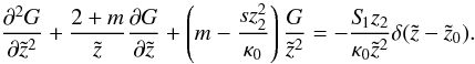 (B.1)With the ansatz
  (B.2)we find the corresponding homogeneous solutions:
 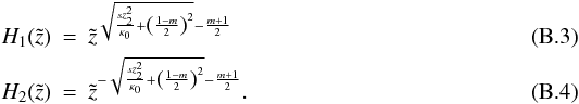 Again, a particular solution can be found utilizing the variation-of-constants method:
 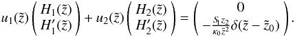 (B.5)The solutions for this linear system of equations are
 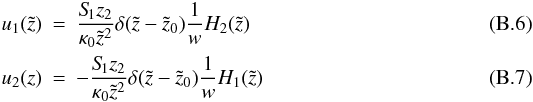 with the Wronskian:
 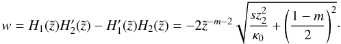 (B.8)A particular solution for Eq. (B.1) is therefore given by
  (B.9)where and are integrals of and .
If we choose 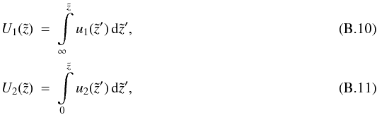 the particular solution reads as
 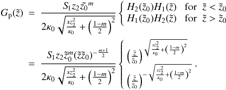 (B.12)Using the relation (5.6.6) from Erdelyi (1954)
 (B.13)we find
 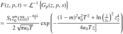 (B.14)as a solution for the time-dependent focused diffusion equation for α = 2.
The equation presented in Earl (1976) looks slightly different because of a different definition of the phase-space density: FEarl = FB0.
Acknowledgments
Partial support by the Deutsche Forschungsgemeinschaft through grant Schl 201/23-1 is gratefully acknowledged.
The work at the University of California, Berkeley, was supported by NASA under contracts NNX08AE34G and NAS5-98033.
The Wind 3D Plasma & Energetic Particle investigation at Berkeley was funded by NASA Grant NNX10AQ31G. R. P. Lin was also supported in part by the WCU grant (No. R31-10016) funded by the Korean Ministry of Education, Science, and Technology.
References
- Agueda, N., Vainio, R., Lario, D., & Sanahuja, B. 2008, ApJ, 675, 1601 [Google Scholar]
- Agueda, N., Lario, D., Vainio, R., et al. 2009, A&A, 507, 981 [NASA ADS] [CrossRef] [EDP Sciences] [Google Scholar]
- Bieber, J. W., Evenson, P., Dröge, W., et al. 2004, ApJ, 601, L103 [Google Scholar]
- Bryant, D. A., Cline, T. L., Desai, U. D., & McDonald, F. B. 1964, NASA Spec. Publ., 50, 289 [NASA ADS] [Google Scholar]
- Dröge, W. 2003, ApJ, 589, 1027 [Google Scholar]
- Dröge, W. 2005, Adv. Space Res., 35, 532 [NASA ADS] [CrossRef] [Google Scholar]
- Dröge, W., & Kartavykh, Y. Y. 2009, ApJ, 693, 69 [NASA ADS] [CrossRef] [Google Scholar]
- Dröge, W., Kartavykh, Y. Y., Klecker, B., & Kovaltsov, G. A. 2010, ApJ, 709, 912 [NASA ADS] [CrossRef] [Google Scholar]
- Dunkel, J., Talkner, P., & Hänggi, P. 2007, Phys. Rev. D, 75, 043001 [NASA ADS] [CrossRef] [Google Scholar]
- Earl, J. A. 1976, ApJ, 205, 900 [NASA ADS] [CrossRef] [Google Scholar]
- Erdelyi, A. 1954, Tables of Integral Transforms (New York: McGraw-Hill), 1 [Google Scholar]
- Heristchi, D., & Amari, T. 1992, Sol. Phys., 142, 209 [NASA ADS] [CrossRef] [Google Scholar]
- Kocharov, L. G., Torsti, J., Vainio, R., & Kovaltsov, G. A. 1996, Sol. Phys., 165, 205 [NASA ADS] [CrossRef] [Google Scholar]
- Lin, R. P., Anderson, K. A., Ashford, S., et al. 1995, Space Sci. Rev., 71, 125 [NASA ADS] [CrossRef] [Google Scholar]
- Meyer, P., Parker, E. N., & Simpson, J. A. 1956, Phys. Rev., 104, 768 [Google Scholar]
- Parker, E. N. 1958, ApJ, 128, 664 [Google Scholar]
- Qin, G., Zhang, M., Dwyer, J. R., & Rassoul, H. K. 2004, ApJ, 609, 1076 [NASA ADS] [CrossRef] [Google Scholar]
- Rossi, B., & Olbert, S. 1970, Introduction to the physics of space (New York: McGraw-Hill) [Google Scholar]
- Ruffolo, D. 1995, ApJ, 442, 861 [NASA ADS] [CrossRef] [Google Scholar]
- Schlickeiser, R., & Shalchi, A. 2008, ApJ, 686, 292 [NASA ADS] [CrossRef] [Google Scholar]
- Schlickeiser, R., Dohle, U., Tautz, R. C., & Shalchi, A. 2007, ApJ, 661, 185 [NASA ADS] [CrossRef] [Google Scholar]
- Schlickeiser, R., Artmann, S., & Dröge, W. 2009, The Open Plasma Physics Journal, 2, 1 [Google Scholar]
- Shalchi, A. 2009, Nonlinear Cosmic Ray Diffusion Theories (Berlin: Springer-Verlag) [Google Scholar]
- Toptygin, I. N. 1985, Cosmic rays in interplanetary magnetic fields (Dordrecht: D. Reidel Publishing Company) [Google Scholar]
All Tables
All Figures
|
Fig. 1 Sketch of the temporal evolution of the spatial intensity distribution of solar energetic particles released instantaneously at T = 0 for α = 1 and m = −2. |
| In the text | |
|
Fig. 2 Sketch of the spatial dependence of the intensity distribution on the magnetic field structure (Eq. (5)) at a given time T = 1 h for α = 1. |
| In the text | |
|
Fig. 3 Sketch of the temporal dependence of the intensity distribution on the magnetic field structure (Eq. (5)) at a given position |
| In the text | |
|
Fig. 4 Sketch of the spatial dependence of the intensity distribution on the spatial power-law dependence of the diffusion coefficient at a given time T = 1 h for m = −2. |
| In the text | |
|
Fig. 5 Sketch of the temporal dependence of the intensity distribution on the spatial power-law dependence of the diffusion coefficient at a given position |
| In the text | |
|
Fig. 6 Sketch of the spatial dependence of the mean free path λ for three different powers. |
| In the text | |
|
Fig. 7 Sketch of the anisotropy-time profile (Eq. (29)) in comparison with the approximation (Eq. (33)) for three different values for α. |
| In the text | |
|
Fig. 8 Anisotropy- and intensity-time profiles for 40 − 512 keV electrons measured with the Wind/3DP instrument in comparison with the theoretically derived profile (19) with the parametervalues listed in Table 1. |
| In the text | |
|
Fig. 9 Energy dependence of the injection function S1 (solid black line with crosses) in comparison with a ∝ |
| In the text | |
|
Fig. 10 Normalized intensity-distance profiles for four different electron energies. vT represents the distance that the electrons cover after their first detection at the given position. |
| In the text | |
|
Fig. 11 Normalized intensity-distance profiles for the three lowest energies of Wind/3DP in comparison with the 511 keV electrons. |
| In the text | |
|
Fig. 12 Anisotropy-distance profiles for four different electron energies. |
| In the text | |
Current usage metrics show cumulative count of Article Views (full-text article views including HTML views, PDF and ePub downloads, according to the available data) and Abstracts Views on Vision4Press platform.
Data correspond to usage on the plateform after 2015. The current usage metrics is available 48-96 hours after online publication and is updated daily on week days.
Initial download of the metrics may take a while.