| Issue |
A&A
Volume 531, July 2011
|
|
|---|---|---|
| Article Number | A173 | |
| Number of page(s) | 13 | |
| Section | The Sun | |
| DOI | https://doi.org/10.1051/0004-6361/201014976 | |
| Published online | 08 July 2011 | |
Online material
Appendix A: Spatial resolution and residual image motion
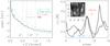 |
Fig. A.1
Spatial resolution. Left: Fourier power as function of spatial frequency. Right: vertical and horizontal cuts through the center of the H2R map shown as inset at the upper left. Gaussian fits to the central brightening are overplotted with red and blue lines, respectively. |
| Open with DEXTER | |
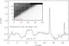 |
Fig. A.2
Position of the limb in the OW map (inset at the upper left in logarithmic scaling). The inclined dash-dotted line in the inset denotes a linear fit to the limb position. The black line denotes an intensity level of 0.25%. The line plot below the inset shows the difference between the dash-dotted line and the actual limb position in arcsec. |
| Open with DEXTER | |
Because observations near the solar limb are usually difficult, especially when one tries to maintain the AO real-time correction, we investigate the achieved spatial resolution. Figure A.1 shows two estimates of the spatial resolution, from the Fourier power as function of the spatial frequency (left) and the extension of an isolated brightening in the H2R map (right). The spatial sampling provides a maximal resolution of 0 6. The Fourier power levels off to a constant value that is indicative of the noise level between 1′′ and 1.5′′. The shape of the curves for different wavelength windows (OW, H-index, fixed wavelength at 396.822 nm) or the difference between H2V and H2R is fairly similar, with slightly enhanced power for the intensity difference measure. A Gaussian fit to the extension of the isolated brightening shown as inset in the right panel yielded a FWHM of 1.5′′ and 1.9′′ on cuts in the horizontal and vertical direction, respectively, with the caveat that the feature presumably will also have an intrinsic spatial extent. The spatial resolution should accordingly be about 1.5′′ or slightly better.
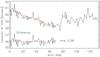 |
Fig. A.3
Location of the limb for one spatial position in the SJ images. The lower part shows the difference between the red straight line and the limb position. |
| Open with DEXTER | |
To determine the residual image motion caused by the variable seeing and uncompensated image shifts, we measured the location of the “white-light” limb in the OW map (inset in Fig. A.2). The limb was defined as the point where the intensity dropped below 4%. We fitted a straight line to the limb location and then derived the difference to the actual limb position at one scan step and the straight line (Fig. A.2). The rms variation of the difference is about 017. Because this is now derived from the spectra after the 13-s integration, it only provides a temporally averaged value of the image motion. We therefore used the individual slit-jaw (SJ) images for a cross-check. The SJ images are taken at the beginning of each scan step with an exposure time below 20 ms; they are thus not influenced by any temporal averaging. We removed the image motion caused by the spatial scanning perpendicular to the slit from the SJ images, and then determined the location of the limb in the individual images, defined again as the position where the intensity drops below 4%. Figure A.3 shows the distance between the limb and the edge of the SJ image for one randomly chosen image row. In addition to a linear trend that could be caused by a slow drift of the AO lock point or a small tilt angle between the POLIS scan mirror and the slit, the limb position in the SJ images fluctuated with an rms amplitude of about 036. The fluctuations of the atmospheric scattering were below a level of 0.25% in the OW map, the map is still fairly homogeneous at this intensity level (black line in the inset of in Fig. A.2), with the distance to the limb being the dominating factor for the residual light level.
Appendix B: Additional example spectra
Figure B.1 shows an example of the multi-lobed profiles found on the disk near a patch of enhanced emission and strong photospheric polarization signal. Figure B.2 shows a series of individual neighboring spectra at a limb distance of 2.5 Mm. The Doppler shift of the absorption core relative to the emission peaks reverses from blue to red shift over a spatial scale of about 1.6′′. The spectra along the slit (Fig. B.3) show the same patterns as those along cuts perpendicular to the limb: a variation of Doppler shifts both in the horizontal direction from scan step to scan step as well as a variation in single cuts along the vertical axis. Figures B.4 and B.5 show the individual profiles of cut no. 2 and the scan step no. 66. In the first case, the distance given at the left of each profile is measured perpendicular to the limb, in the latter case it only reflects the location along the slit.
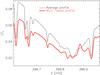 |
Fig. B.1
Ca profile with more than two reversals (thick red). The thin black line shows the average profile for comparison. |
| Open with DEXTER | |
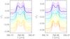 |
Fig. B.2
Individual spectra at a limb distance of 2.5 Mm. Left: spectra from x = 4.5′′ to 8.4′′. Thick lines indicate profiles with large shifts. Right: same from x = 9.3′′ to 13.5′′. The position values refer to the spatial scale given in Fig. 7. |
| Open with DEXTER | |
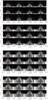 |
Fig. B.3
Spectra along the slit around the scan step 21 (top panel), step 37 (second panel), step 53 (third panel), and step 66 (bottom panel). The scan step of each cut along the slit is given at the lower left of each panel, increasing from left to right and from bottom up. The y-axis gives the distance along the cut, the limb is thus located at varying positions. The vertical white line denotes the rest wavelength of Ca ii H. |
| Open with DEXTER | |
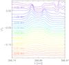 |
Fig. B.4
Spectra of cut no. 2 (see Fig. 3) with increasing limb distance. The limb is at the top, each third profile is labeled with its corresponding height. |
| Open with DEXTER | |
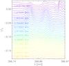 |
Fig. B.5
Spectra of scan step no. 66 (see Fig. 3) with increasing position along the slit. The limb is at the top, each third profile is labeled with its corresponding height. |
| Open with DEXTER | |
© ESO, 2011
Current usage metrics show cumulative count of Article Views (full-text article views including HTML views, PDF and ePub downloads, according to the available data) and Abstracts Views on Vision4Press platform.
Data correspond to usage on the plateform after 2015. The current usage metrics is available 48-96 hours after online publication and is updated daily on week days.
Initial download of the metrics may take a while.