| Issue |
A&A
Volume 527, March 2011
|
|
|---|---|---|
| Article Number | A26 | |
| Number of page(s) | 36 | |
| Section | Cosmology (including clusters of galaxies) | |
| DOI | https://doi.org/10.1051/0004-6361/201015621 | |
| Published online | 20 January 2011 | |
Online material
Appendix A: Three-dimensional number density-intrinsic shear correlation function
In this appendix, we derive the three-dimensional number density-intrinsic shear (gI) correlation function, detail the inclusion of photometric redshift scatter into the formalism, and establish an approximate relation between the three-dimensional correlation function and the angular power spectrum.
A.1. Correlation function for exact redshifts
We define the three-dimensional correlation function between the galaxy density
contrast δg and the radial intrinsic shear
γI, + as  (A.1)for a given mean
redshift z of the galaxy pairs correlated. Here we introduced a
three-dimensional comoving separation vector x which has
a line-of-sight component Π ≡ x ∥ . Its transverse
components are denoted by
x ⊥ , with
modulus
rp ≡ | x ⊥ | .
The first argument of both δg and
γI, + denotes the position on the sky, the second the
position along the line of sight, and the third quantifies the epoch, given in terms
of the redshift. Note that a line-of-sight separation Π ≠ 0 implies that
δg and γI, + are not
measured at precisely the same epoch, contrary to what we have written in (A.1). However, as Π is small compared to
the comoving distance χ(z) to the galaxies under
consideration, this approximation holds to good accuracy.
(A.1)for a given mean
redshift z of the galaxy pairs correlated. Here we introduced a
three-dimensional comoving separation vector x which has
a line-of-sight component Π ≡ x ∥ . Its transverse
components are denoted by
x ⊥ , with
modulus
rp ≡ | x ⊥ | .
The first argument of both δg and
γI, + denotes the position on the sky, the second the
position along the line of sight, and the third quantifies the epoch, given in terms
of the redshift. Note that a line-of-sight separation Π ≠ 0 implies that
δg and γI, + are not
measured at precisely the same epoch, contrary to what we have written in (A.1). However, as Π is small compared to
the comoving distance χ(z) to the galaxies under
consideration, this approximation holds to good accuracy.
Following Hirata & Seljak (2004), the
radial component of the intrinsic shear is measured with respect to
x ⊥ , and
without loss of generality we can choose the coordinate system such that
γI, + = γI,1. Note that in
the majority of weak lensing studies γ + is defined as
the tangential component of the shear. Measuring radial instead of tangential
alignment implies a change of sign, so that e.g. the galaxy-galaxy lensing signal
which we consider is negative. Denoting Fourier variables by a tilde, one can
construct in analogy to the matter density contrast a three-dimensional intrinsic
convergence δI12 via
 (A.2)where
ϕ is the polar angle of
k ⊥ , i.e. the projection of the wave
vector onto the plane of the sky. We will denote the line-of-sight component of
k by k ∥ .
(A.2)where
ϕ is the polar angle of
k ⊥ , i.e. the projection of the wave
vector onto the plane of the sky. We will denote the line-of-sight component of
k by k ∥ .
Then one can write the correlation function by Fourier transforming (A.1) as  (A.3)Inserting
the definition of the three-dimensional gI power spectrum,
(A.3)Inserting
the definition of the three-dimensional gI power spectrum,
 (A.4)and subsequently
integrating (A.3) over
k′ yields
(A.4)and subsequently
integrating (A.3) over
k′ yields
 (A.5)where
in order to arrive at the third equality, the definition of the second-order Bessel
function of the first kind was used. In this derivation it was implicitly assumed that
the intrinsic shear field does not feature B-modes, as is for instance the case for
the linear alignment paradigm.
(A.5)where
in order to arrive at the third equality, the definition of the second-order Bessel
function of the first kind was used. In this derivation it was implicitly assumed that
the intrinsic shear field does not feature B-modes, as is for instance the case for
the linear alignment paradigm.
One can now integrate over the line of sight, making use of the definition of the
Dirac delta-distribution, to obtain the projected gI correlation function as employed
by Mandelbaum et al. (2006), Hirata et al. (2007), and Mandelbaum et al. (2010), 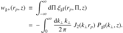 (A.6)Real
data cannot provide the correlation function for arbitrarily large line-of-sight
separations, so that a truncation of the integral in (A.6) is necessary. This formula is still applicable if one can
stack observations for all values of Π for which galaxy pairs carry a signal. While
this can easily be achieved for spectroscopic observations, photometric redshift
scatter smears the signal in Π such that a cut-off Πmax needs to be taken
into account explicitly in the modelling. Of course it would be possible to compute
the observed correlations out to very large Πmax, but this way many
uncorrelated galaxy pairs would enter the correlation function, thereby decreasing the
signal-to-noise dramatically.
(A.6)Real
data cannot provide the correlation function for arbitrarily large line-of-sight
separations, so that a truncation of the integral in (A.6) is necessary. This formula is still applicable if one can
stack observations for all values of Π for which galaxy pairs carry a signal. While
this can easily be achieved for spectroscopic observations, photometric redshift
scatter smears the signal in Π such that a cut-off Πmax needs to be taken
into account explicitly in the modelling. Of course it would be possible to compute
the observed correlations out to very large Πmax, but this way many
uncorrelated galaxy pairs would enter the correlation function, thereby decreasing the
signal-to-noise dramatically.
Instead, we proceed from (A.5) by
assuming that ξgI is a real function, and write
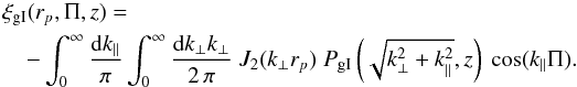 (A.7)As
can be seen from this equation, ξgI is an even function in
both rp and Π, so that it is sufficient
to compute just one quadrant. Note that by definition
rp ≥ 0, whereas Π can also attain
negative values.
(A.7)As
can be seen from this equation, ξgI is an even function in
both rp and Π, so that it is sufficient
to compute just one quadrant. Note that by definition
rp ≥ 0, whereas Π can also attain
negative values.
 |
Fig. A.1
Three-dimensional gI correlation function as a function of comoving line-of-sight separation Π and comoving transverse separation rp at z ≈ 0.5. Contours are logarithmically spaced between 10-2 (yellow) and 10-6 (black) with three lines per decade. Top panel: applying a Gaussian photometric redshift scatter of width 0.02. Bottom panel: assuming exact redshifts. Note the largely different scaling of the ordinate axes. The galaxy bias has been set to unity, and (6) with SuperCOSMOS normalisation has been used to model PδI in both cases. Redshift-space distortions have not been taken into account. |
| Open with DEXTER | |
Equation (A.7) yields the three-dimensional gI correlation function for exact or, to good approximation, spectroscopic redshifts. For the model described in Sect. 4 with SuperCOSMOS normalisation and bg = 1, we plot ξgI(rp,Π,z) for z ≈ 0.5 in Fig. A.1, bottom panel. As expected, the correlation is strongest for small separation, in particular for |Π| close to zero. If spectroscopic data is available, essentially all information is captured when a cut-off Πmax = 60 h-1 Mpc is used in the integration (A.6), as e.g. in Mandelbaum et al. (2010). Due to the definition (A.1), the gI correlation function measures the radial alignment of the galaxy shape with respect to the separation vector of the galaxy pair considered. Therefore the correlation function vanishes for all Π at rp = 0 since then the separation vector points along the of sight. Note that the contours do not approach the Π = 0-axis asymptotically, but cross this line at some value of rp, as expected for a differentiable correlation function. Throughout these considerations we have not taken the effect of redshift-space distortions into account.
A.2. Incorporating photometric redshifts
Photometric redshift errors cause the observed correlation function to be a “smeared”
version of (A.7), introducing a spread
especially along the line of sight but to a lesser extent also in transverse
separation (because an uncertain redshift is used to convert angular separation to
physical separation). If we denote quantities determined via photometric redshifts by
a bar, the actually measured three-dimensional correlation function reads
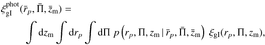 (A.8)where
zm denotes the mean redshift of the galaxy samples used
for the number density and the shape measurement. Here, p is the
probability distribution of the true values of
rp, Π, and
zm, given photometric redshift estimates of these
quantities. In words, (A.8) means that
in order to obtain the observed correlation function, we integrate over
ξgI as given in (A.7), weighted by the probability that the true values for
separations and redshift actually correspond to the estimates based on photometric
redshifts.
(A.8)where
zm denotes the mean redshift of the galaxy samples used
for the number density and the shape measurement. Here, p is the
probability distribution of the true values of
rp, Π, and
zm, given photometric redshift estimates of these
quantities. In words, (A.8) means that
in order to obtain the observed correlation function, we integrate over
ξgI as given in (A.7), weighted by the probability that the true values for
separations and redshift actually correspond to the estimates based on photometric
redshifts.
The direct observables for this measurement are the redshifts of the two galaxy
samples under consideration, z1 and
z2, and their angular separation θ. The
sets of variables
(z1,z2,θ)
and (rp,Π,zm)
are related via a bijective transformation. Writing (A.8) in terms of the other set of variables, one obtains
 (A.9)In
the second step it was assumed that the probability distributions of
z1, z2, and
θ are mutually independent, and that θ is exactly
known, i.e.
(A.9)In
the second step it was assumed that the probability distributions of
z1, z2, and
θ are mutually independent, and that θ is exactly
known, i.e.  .
We have introduced different redshift probability distributions for the galaxy sample
with number density information pn and
the one with shape information pϵ. All
quantities related to photometric redshifts have been expressed in terms of the
arguments of the correlation function on the left-hand-side.
.
We have introduced different redshift probability distributions for the galaxy sample
with number density information pn and
the one with shape information pϵ. All
quantities related to photometric redshifts have been expressed in terms of the
arguments of the correlation function on the left-hand-side.
We make use of the following approximate relations between the two triples of
variables, 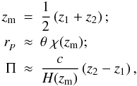 (A.10)where
H(z) is the Hubble parameter. Note that the same
transformations have been used to bin the observational data in terms of redshift,
transverse and line-of-sight separation. With this equation for Π, in combination with
the assignment of probability distributions in (A.9), we have introduced the convention that Π > 0 means
that the galaxy from the density sample is at lower redshift than the galaxy from the
shape sample. If and only if the distributions for the density and the shape sample
are identical, which we assume throughout this work, the correlation function remains
symmetric with respect to Π, i.e.
(A.10)where
H(z) is the Hubble parameter. Note that the same
transformations have been used to bin the observational data in terms of redshift,
transverse and line-of-sight separation. With this equation for Π, in combination with
the assignment of probability distributions in (A.9), we have introduced the convention that Π > 0 means
that the galaxy from the density sample is at lower redshift than the galaxy from the
shape sample. If and only if the distributions for the density and the shape sample
are identical, which we assume throughout this work, the correlation function remains
symmetric with respect to Π, i.e.  .
.
With these equations at hand, one can also write down the inverse transformation of
(A.10), which is needed to evaluate
(A.9), 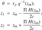 (A.11)Then
(A.9) can be expressed as
(A.11)Then
(A.9) can be expressed as
 (A.12)Note
that the absolute value for
z2 − z1 has been introduced
in the second argument of ξgI, which is possible since it
is an even function in this argument. The integrals in (A.12) run over the full range of spectroscopic (exact) redshifts.
As a consequence,
| z2 − z1 | in the second
argument of ξgI can obtain relatively large values,
leading to very large Π ≫ 100 h-1 Mpc. However, the
spectroscopic ξgI becomes very small for large Π, so that
the integrand in (A.12) can safely be
set to zero in this case.
(A.12)Note
that the absolute value for
z2 − z1 has been introduced
in the second argument of ξgI, which is possible since it
is an even function in this argument. The integrals in (A.12) run over the full range of spectroscopic (exact) redshifts.
As a consequence,
| z2 − z1 | in the second
argument of ξgI can obtain relatively large values,
leading to very large Π ≫ 100 h-1 Mpc. However, the
spectroscopic ξgI becomes very small for large Π, so that
the integrand in (A.12) can safely be
set to zero in this case.
Still, any sizeable photometric redshift scatter leads to a considerable spread of
the three-dimensional correlation function in Π, as can be seen in Fig. A.1. Assuming a Gaussian photometric redshift
scatter with width 0.02 around every true redshift, the strong signal concentrated at
small Π and
rp ≲ 10 h-1 Mpc
in the spectroscopic case is scattered along the line of sight, so that the values of
 at
Π > 200 h-1 Mpc are still more than a per cent
of those at Π = 0 for any rp. In
contrast, we find that the net scatter of signal between different transverse
separations is negligible. Hence, in principle the projected correlation function
(A.6) does not change when using
photometric instead of spectroscopic redshift information as long as the complete
range of Π for which a signal is measured enters the line-of-sight integration.
However, in practice the line-of-sight integral has to be truncated for reasons of a
good signal-to-noise ratio, so that in the case of photometric redshifts part of the
signal is lost. Therefore it is crucial to repeat the same steps applied to the data
also to the model and use the same cut-off Πmax in (A.6).
at
Π > 200 h-1 Mpc are still more than a per cent
of those at Π = 0 for any rp. In
contrast, we find that the net scatter of signal between different transverse
separations is negligible. Hence, in principle the projected correlation function
(A.6) does not change when using
photometric instead of spectroscopic redshift information as long as the complete
range of Π for which a signal is measured enters the line-of-sight integration.
However, in practice the line-of-sight integral has to be truncated for reasons of a
good signal-to-noise ratio, so that in the case of photometric redshifts part of the
signal is lost. Therefore it is crucial to repeat the same steps applied to the data
also to the model and use the same cut-off Πmax in (A.6).
A.3. Relation to angular power spectra
We now derive a relation between the three-dimensional gI correlation function in the
presence of photometric redshift scatter and the angular power spectrum, which proves
most convenient to compute in
practice. Inserting (A.5) into (A.12), one can write
 (A.13)where
we employed
zm = (z1 + z2)/2
as a shorthand notation. Making use of
(A.13)where
we employed
zm = (z1 + z2)/2
as a shorthand notation. Making use of  ,
see (A.11), and defining the angular
frequency
,
see (A.11), and defining the angular
frequency  , one
obtains
, one
obtains  (A.14)We
then transform the integration variables
{z1,z2} to
{zm,Δz ≡ z2 − z1}.
Note that the determinant of the Jacobian of this transformation is unity. We apply
Limber’s approximation, which in this case can be written as
(A.14)We
then transform the integration variables
{z1,z2} to
{zm,Δz ≡ z2 − z1}.
Note that the determinant of the Jacobian of this transformation is unity. We apply
Limber’s approximation, which in this case can be written as
 (A.15)Here
we have assumed that the two redshift probability distributions are sufficiently broad
and have similar forms, so that an evaluation at zm
instead of zm ± Δz/2 does not change
the results significantly. Since the photometric redshifts on which the distributions
are conditional encapsulate the dependence of on the
line-of-sight separation Π, we do not extend this approximation to the second
argument. Equation (A.14) thereby
simplifies to
(A.15)Here
we have assumed that the two redshift probability distributions are sufficiently broad
and have similar forms, so that an evaluation at zm
instead of zm ± Δz/2 does not change
the results significantly. Since the photometric redshifts on which the distributions
are conditional encapsulate the dependence of on the
line-of-sight separation Π, we do not extend this approximation to the second
argument. Equation (A.14) thereby
simplifies to  (A.16)where
in order to arrive at the second equality, we integrated over Δz. The
resulting Dirac delta-distribution renders the k ∥
integration trivial. Making use of the expressions
(A.16)where
in order to arrive at the second equality, we integrated over Δz. The
resulting Dirac delta-distribution renders the k ∥
integration trivial. Making use of the expressions
 and
p(z) = p(χ) dχ/dz,
one obtains the result
and
p(z) = p(χ) dχ/dz,
one obtains the result 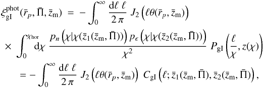 (A.17)where
in the last step we implicitly defined the projected gI auto-correlation power
spectrum CgI. In addition to the angular frequency, we
have written the photometric redshifts
(A.17)where
in the last step we implicitly defined the projected gI auto-correlation power
spectrum CgI. In addition to the angular frequency, we
have written the photometric redshifts  and
and  ,
which characterise the redshift distributions entering
CgI, explicitly as arguments. Note that Limber equations,
such as (5), in general hold only
approximately, the range of validity being the more limited the narrower the kernels
in the line-of-sight integration (e.g. Simon
2007).
,
which characterise the redshift distributions entering
CgI, explicitly as arguments. Note that Limber equations,
such as (5), in general hold only
approximately, the range of validity being the more limited the narrower the kernels
in the line-of-sight integration (e.g. Simon
2007).
We have verified that the calculations of the three-dimensional gI correlation
function according to (A.12) and
(A.17) agree within the numerical
accuracy. The latter can be computed much more efficiently by computing the angular
power spectrum via Limber’s equation and then using Hankel transformations to obtain
the correlation function  via (A.17), employing the transformation (A.10). One can proceed likewise to obtain
analogous expressions for the gg signal. Galaxy-galaxy lensing vanishes if the density
field probed by the galaxy distribution and the source galaxies on whose images the
gravitational shear is measured are located at exactly the same redshift. Thus one
cannot proceed with the same formalism as used to derive the gI contribution (see the
assumptions underlying the definition (A.1)), but must instead incorporate redshift probability distributions from
the start, again arriving at an expression analogous to (A.17).
via (A.17), employing the transformation (A.10). One can proceed likewise to obtain
analogous expressions for the gg signal. Galaxy-galaxy lensing vanishes if the density
field probed by the galaxy distribution and the source galaxies on whose images the
gravitational shear is measured are located at exactly the same redshift. Thus one
cannot proceed with the same formalism as used to derive the gI contribution (see the
assumptions underlying the definition (A.1)), but must instead incorporate redshift probability distributions from
the start, again arriving at an expression analogous to (A.17).
Appendix B: Redshift dependence of the linear alignment model
In this appendix we re-derive the redshift dependence of the linear alignment model, obtaining a different result than Hirata & Seljak (2004), but being in full agreement with Hirata & Seljak (2010). Practically all attempts at constructing a physical description for intrinsic alignments are based on the linear alignment model originally suggested by Catelan et al. (2001). They assumed that the shape of the luminous part of a galaxy exactly follows the shape of its host halo, and that the ellipticity of the latter is determined by the local tidal gravitational field of the large-scale structure.
The simplest possible form allowed by the assumptions made above is a linear relation
between the intrinsic shear and the gravitational field, given by (Catelan et al. 2001)  (B.1)where
we wrote the normalisation in the notation of Hirata
& Seljak (2004) in which C1 is an arbitrary
constant. The partial derivatives are with respect to comoving coordinates, and
Φp(x) ≡ Φ(x,zp)
denotes the “primordial” potential, i.e. the linear gravitational potential evaluated at
the epoch of galaxy formation, at a redshift zp well within
the matter-dominated era. For ease of notation we have omitted a smoothing of the
gravitational potential on galactic scales in (B.1) which can be implemented by a simple cut-off of high wavenumbers in
Fourier space, see Hirata & Seljak
(2004). These authors used the relations (B.1) in their derivation of the intrinsic alignment power spectra
for the linear alignment model, which we closely follow.
(B.1)where
we wrote the normalisation in the notation of Hirata
& Seljak (2004) in which C1 is an arbitrary
constant. The partial derivatives are with respect to comoving coordinates, and
Φp(x) ≡ Φ(x,zp)
denotes the “primordial” potential, i.e. the linear gravitational potential evaluated at
the epoch of galaxy formation, at a redshift zp well within
the matter-dominated era. For ease of notation we have omitted a smoothing of the
gravitational potential on galactic scales in (B.1) which can be implemented by a simple cut-off of high wavenumbers in
Fourier space, see Hirata & Seljak
(2004). These authors used the relations (B.1) in their derivation of the intrinsic alignment power spectra
for the linear alignment model, which we closely follow.
In a first step, the primordial gravitational potential is related to the matter
density contrast via the Poisson equation  (B.2)where
 denotes the
comoving Laplacian. This expression is Fourier-transformed, yielding
denotes the
comoving Laplacian. This expression is Fourier-transformed, yielding  (B.3)The growth factor
D(z) quantifies the dependence of the matter density
contrast on redshift in the limit of linear structure formation, and is normalised to
D(z) = (1 + z)-1 during
matter domination (Hirata & Seljak
2004)13. Restricting (B.3) to linear scales, one obtains the ratio
(B.3)The growth factor
D(z) quantifies the dependence of the matter density
contrast on redshift in the limit of linear structure formation, and is normalised to
D(z) = (1 + z)-1 during
matter domination (Hirata & Seljak
2004)13. Restricting (B.3) to linear scales, one obtains the ratio
 (B.4)where in the
last step we made use of the fact that zp lies in the
matter-dominated era. Inserting (B.4)
into (B.3), and considering the linear
regime, one arrives at the relation between primordial potential and linear matter
density contrast,
(B.4)where in the
last step we made use of the fact that zp lies in the
matter-dominated era. Inserting (B.4)
into (B.3), and considering the linear
regime, one arrives at the relation between primordial potential and linear matter
density contrast,  (B.5)This expression
differs from the result given in Hirata & Seljak
(2004), Eq. (14), by an additional factor
(1 + z)-2. This discrepancy was also found in other
re-derivations (Hirata & Seljak 2010;
Bean, Laszlo; priv. comm.).
(B.5)This expression
differs from the result given in Hirata & Seljak
(2004), Eq. (14), by an additional factor
(1 + z)-2. This discrepancy was also found in other
re-derivations (Hirata & Seljak 2010;
Bean, Laszlo; priv. comm.).
Hirata & Seljak (2004) inserted their
Eq. (14) into (B.1) and then computed
the three-dimensional intrinsic shear (II) power spectrum and the intrinsic shear-matter
cross-power spectrum. Neglecting source clustering but otherwise following their steps
in exact analogy, we obtain  where
in this work we use the full nonlinear matter power spectrum on the right-hand side
instead of the linear power spectrum, as written here in the original form of the linear
alignment model. If Hirata & Seljak
(2004), Eq. (14), were employed instead of (B.5), (B.6) would
have an additional term (1 + z)4, and (B.7) an additional term
(1 + z)2, in the numerator. These modifications would
correspond to a shift by − 2 in ηother in our models (19) and (23).
where
in this work we use the full nonlinear matter power spectrum on the right-hand side
instead of the linear power spectrum, as written here in the original form of the linear
alignment model. If Hirata & Seljak
(2004), Eq. (14), were employed instead of (B.5), (B.6) would
have an additional term (1 + z)4, and (B.7) an additional term
(1 + z)2, in the numerator. These modifications would
correspond to a shift by − 2 in ηother in our models (19) and (23).
Appendix C: Volume density and luminosities of red galaxies
To make realistic predictions for the intrinsic alignment contamination of cosmic shear surveys, we must specify, at each redshift, the distribution of galaxy luminosities that enter (19). Since this intrinsic alignment model only holds for red galaxies, we additionally must estimate the fraction of early-type galaxies in the total weak lensing population as a function of redshift. In this paper, both quantities are determined using fits to the observed luminosity functions given in Faber et al. (2007). In this appendix, we present technical details about these calculations, assess the sensitivity of our results to this particular luminosity function choice, and provide data that can be used to forecast the intrinsic alignment contamination of other cosmic shear surveys (with different limiting magnitudes) besides that discussed in the main text. In all cases, we are extrapolating the luminosity functions to fainter magnitudes at a given redshift relative to the samples used to determine the luminosity function.
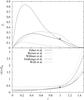 |
Fig. C.1
Red galaxy fraction fr (top panel) and mean luminosity of red galaxies (bottom panel) as a function of redshift for a magnitude limit rlim = 25. We compare the results for the sets of luminosity functions provided by Faber et al. (2007, black solid curves), Brown et al. (2007, dark grey solid curves), Willmer et al. (2006, light grey solid curves), Giallongo et al. (2005, black dotted curves), and Wolf et al. (2003, grey dotted curves). The results for Faber et al. (2007) luminosity functions used with the value of B − r expected at z = 1 are indicated by the cross in each panel. |
| Open with DEXTER | |
We employ the Schechter luminosity function parameters for red galaxies from Faber et al. (2007), where φ∗ and M∗ are given as a function of redshift, and where the faint-end slope is fixed at α = − 0.5. While we consistently use magnitudes in the r band, Faber et al. (2007) determine M∗ in the B band. Therefore we the estimate rest-frame B − r colour from the tables provided in Fukugita et al. (1995), finding B − r = 1.32 for ellipticals. This conversion from B to r takes into account that Faber et al. (2007) give B band magnitudes in the Vega-based system, whereas this work uses AB magnitudes throughout. Furthermore, we have assumed r ≈ r′, where r′ is the filter listed by Fukugita et al. (1995). This assumption should hold to good accuracy14 for typical colours of the galaxies in our samples, i.e. 0.2 ≲ r − i ≲ 0.6.
For early-type galaxies, B − r shows little evolution between z = 0 and z ~ 1 (Bruzual & Charlot 2003), so we assume the rest-frame colour to be constant in this redshift range, which we check via the following procedure. Since the Sloan g filter covers a similar wavelength range to the B band (although the peaks of the transmission curves differ, see Fukugita et al. 1995 for details), we use the evolution of g − r as determined from the Wake et al. (2006) templates as an approximation for the redshift dependence of B − r. We find a shift of 0.15 mag from z = 0 to z = 1, which has significantly less effect on our results than employing different observational results for luminosity functions, see Fig. C.1 and the corresponding discussion below. Finally, we correct for the fact that Faber et al. (2007) have computed absolute magnitudes assuming a Hubble parameter h = 0.7 while we give absolute magnitudes in terms of h = 1.
 |
Fig. C.2
Comoving volume number density of red galaxies nV,r and mean luminosity ⟨L⟩/L0 of red galaxies as a function of limiting magnitude rlim and redshift z. Left panel: comoving volume number density of red galaxies nV,r in units of 10-4 Mpc-3. Contour values range between 10-3 in the upper left and 50 at the bottom. In the upper left corner of the panel nV,r ≈ 0. Right panel: mean r band luminosity. Contour values range between 0.16 in the lower part to 5 in the upper left corner. In both panels the red dashed line marks the values for rlim = 25, the limiting magnitude we employ in our calculations. Decades in contour values are indicated by the black solid lines. |
| Open with DEXTER | |
With all of these caveats, the limiting absolute B band magnitude at
redshift z for a given apparent magnitude limit in the
r band is given by  (C.1)where
kr,red(z) is the
k-correction of red galaxies for the r band (Wake et al. 2006). In line with our convention for
absolute magnitudes, the luminosity distance
DL is computed with
h = 1. If absolute magnitudes are given for other values of the Hubble
parameter, like e.g. in Faber et al. (2007), we
convert these accordingly. The limiting absolute magnitude from (C.1) can then be transformed into the
minimum luminosity entering (27)
and (28),
(C.1)where
kr,red(z) is the
k-correction of red galaxies for the r band (Wake et al. 2006). In line with our convention for
absolute magnitudes, the luminosity distance
DL is computed with
h = 1. If absolute magnitudes are given for other values of the Hubble
parameter, like e.g. in Faber et al. (2007), we
convert these accordingly. The limiting absolute magnitude from (C.1) can then be transformed into the
minimum luminosity entering (27)
and (28), 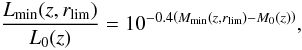 (C.2)where
M0(z) denotes the rest-frame absolute
magnitude − 22, evolution-corrected to redshift z using the redshift
dependence of M∗ from Faber et al. (2007), which is given by − 1.2z. Note that
this dependence accounts for the redshift evolution in the B band, but
since B − r is nearly constant as a function
z, we can also apply the correction (to good approximation) to
r band magnitudes. Denoting the luminosity corresponding to
M∗ by L∗, we obtain for
(28) the expression
(C.2)where
M0(z) denotes the rest-frame absolute
magnitude − 22, evolution-corrected to redshift z using the redshift
dependence of M∗ from Faber et al. (2007), which is given by − 1.2z. Note that
this dependence accounts for the redshift evolution in the B band, but
since B − r is nearly constant as a function
z, we can also apply the correction (to good approximation) to
r band magnitudes. Denoting the luminosity corresponding to
M∗ by L∗, we obtain for
(28) the expression  (C.3)where the incomplete
Gamma function
(C.3)where the incomplete
Gamma function  was
introduced. Analogously, we arrive at
was
introduced. Analogously, we arrive at  (C.4)for
the comoving volume density of red galaxies entering (27).
(C.4)for
the comoving volume density of red galaxies entering (27).
In addition to the luminosity functions from Faber et al. (2007), we also consider fitted Schechter parameters presented in Giallongo et al. (2005), as well as the sets of luminosity functions published by Wolf et al. (2003), Willmer et al. (2006), and Brown et al. (2007). We determine fit functions to the redshift dependence of both M∗ and φ∗ for the latter three works because we have to extrapolate beyond the range of redshift analysed therein. We use linear functions for M∗ and various functional forms with two to three fit parameters for φ∗, but note that since the fits rely on only five to six data points, the extrapolation has considerable uncertainty. All five references give B band luminosity functions, but the magnitude system and the convention for h vary, as well as the redshift ranges covered and the definition of red galaxies.
In Fig. C.1 the red galaxy fraction fr and the mean luminosity ⟨L⟩/L0 for rlim = 25 are plotted as a function of redshift, making use of the different luminosity functions. We find fair agreement between the results based on Faber et al. (2007) and Brown et al. (2007), while the mean luminosities derived from Willmer et al. (2006) already deviate considerably at high z although Faber et al. (2007) and Willmer et al. (2006) partly use the same data. The Wolf et al. (2003) luminosity functions produce significantly lower fr and higher ⟨L⟩ at low redshifts which is caused by the very different value for the faint end slope, α = + 0.52. We note that one of the three fields chosen by Wolf et al. (2003) contained two massive galaxy clusters, so that the large-scale structure in this field could strongly influence the luminosity function in particular of early-type galaxies. However, small red galaxy fractions can be compensated by higher luminosities in (19), so that even the Wolf et al. (2003) luminosity functions may yield intrinsic alignment signals of similar magnitude to the results of e.g. Faber et al. (2007).
Mean luminosity of red galaxies and comoving volume number density of red galaxies as a function of redshift and limiting r band magnitude rlim.
Applying the formalism to luminosity functions from Giallongo et al. (2005), we obtain very high fr at low redshift, which is clearly inconsistent with the other observations. The red galaxy sample used for the fits of Giallongo et al. (2005) is very small and contains only galaxies with z > 0.4. While the resulting fit function captures the pronounced decrease in number density for high redshifts that Giallongo et al. (2005) observe, it can obviously not be used at z ≲ 0.4. In conclusion, we find that the sets of luminosity functions by Faber et al. (2007) who jointly analyse galaxy samples from four different surveys produce reasonable red galaxy fractions and luminosities although the uncertainty in the values of fr and ⟨L⟩ at any given redshift is still large.
In Fig. C.2, the comoving volume density of red galaxies nV,r and the mean luminosity of red galaxies in terms of L0 are plotted as a function of both rlim and redshift, using the default set of luminosity functions from Faber et al. (2007). For a fixed magnitude limit, ⟨L⟩ increases with redshift while nV,r decreases strongly at high redshifts. Both tendencies are more pronounced if the apparent magnitude limit is brighter. At low redshift, e.g. for z ≲ 0.3 at rlim = 25, a large number of faint blue galaxies are above the magnitude limit and cause fr to diminish for z approaching zero (see Fig. C.1) although nV,r continues to increase. This behaviour might change when explicitly taking into account the size cuts inherent to weak lensing surveys, but in any case, galaxies at these low redshifts constitute only a small fraction of the total survey volume and are expected to have a low luminosity and hence low intrinsic alignment signal on average, so they are unlikely to affect our results severely.
The data shown in Fig. C.2, with the corresponding numbers collected in Table C.1, can be used in combination with the intrinsic alignment model fits presented in Sect. 5.5 to predict the effect of intrinsic alignments on cosmic shear surveys. The mean luminosity as a function of redshift for a given magnitude limit rlim can be inserted into the luminosity term in (19), which constitutes a fair approximation as long as values of β close to unity (which includes our best-fit value β = 1.13) are probed. Together with an overall redshift distribution ptot(z) for the cosmic shear survey under consideration, nV,r can be read off and used with (27) to compute the fraction of red galaxies as a function of redshift. Again, we emphasise the limitations of this approach which relies on a substantial amount of extrapolation in luminosity, especially for fainter limiting magnitudes, and which is subject to the large intrinsic uncertainty in the different sets of luminosity functions.
© ESO, 2011
Current usage metrics show cumulative count of Article Views (full-text article views including HTML views, PDF and ePub downloads, according to the available data) and Abstracts Views on Vision4Press platform.
Data correspond to usage on the plateform after 2015. The current usage metrics is available 48-96 hours after online publication and is updated daily on week days.
Initial download of the metrics may take a while.