<!DOCTYPE html PUBLIC "-//W3C//DTD XHTML 1.0 Transitional//EN">
<html xmlns:xlink="http://www.w3.org/1999/xlink" xmlns:mml="http://www.w3.org/1998/Math/MathML">
<link rel="stylesheet" type="text/css" href="../../../CSS_FULL/edps_full.css">
<body><div id="contenu_olm">

<!-- DOI: 10.1051/0004-6361/201014387 -->

<h2 class="sec">Online Material</h2>

<h2 class="sec"><a name="SECTION000100000000000000000"></a> <A NAME="numsol"></A>
Appendix A: Construction of the models  by an iterative procedure
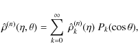
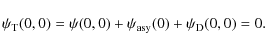
</h2>

<p>Equation (<a href="/articles/aa/full_html/2010/11/aa14387-10/aa14387-10.html#poishalo">18</a>), with the boundary conditions
(<a href="/articles/aa/full_html/2010/11/aa14387-10/aa14387-10.html#boundary">20</a>), is solved by means of a modified version of the
iterative procedure presented earlier by Prendergast &amp; Tomer (<A NAME="aaref25"></A><a href="/articles/aa/full_html/2010/11/aa14387-10/aa14387-10.html#Prendergast1970">1970</a>) in view of a completely different problem (the
study of nonspherical models for rotating elliptical galaxies).
It is based on the classical expansion in Legendre polynomials, a
natural approach in the case of axisymmetric systems. However, the
original method is viable only for gravitational potentials that
are regular at large radii. In contrast, in our model, the
potential of the isothermal halo diverges at large radii. This
difficulty has been overcome by separating the potential of the
dark matter halo into two different parts: a regular part, which
converges to finite values at large radii, and a divergent one,
which follows the asymptotic prescription of Eq.&nbsp;(<a href="/articles/aa/full_html/2010/11/aa14387-10/aa14387-10.html#boundary">20</a>).
Below we provide the details of the technique developed in the
present paper.
Here it is convenient to work with standard spherical coordinates

<!-- MATH: $(r, \phi, \theta)$ -->
<IMG SRC="img186.png" ALT="$(r, \phi, \theta)$" ALIGN="MIDDLE" BORDER="0" HEIGHT="26" WIDTH="43">
and their dimensionless analogue 
<!-- MATH: $(\eta, \phi,
\theta)$ -->
<IMG SRC="img187.png" ALT="$(\eta, \phi,
\theta)$" ALIGN="MIDDLE" BORDER="0" HEIGHT="26" WIDTH="46">.
We start by recalling briefly the method devised by
Prendergast &amp; Tomer (<a href="/articles/aa/full_html/2010/11/aa14387-10/aa14387-10.html#Prendergast1970">1970</a>). The solution of the two-dimensional Poisson
equation
<br></p><p></p>
<DIV ALIGN="CENTER">

<!-- MATH: \begin{equation}
\nabla^2\psi(\eta,\theta)=\hat\rho\left[\eta, \theta; \psi(\eta, \theta)\right]
\end{equation} -->
<TABLE ALIGN="CENTER" WIDTH="100%">
<tbody><tr VALIGN="MIDDLE"><td ALIGN="CENTER" nowrap="nowrap"><A NAME="pois2d"></A><IMG SRC="img188.png" ALT="\begin{displaymath}\nabla^2\psi(\eta,\theta)=\hat\rho\left[\eta, \theta; \psi(\eta, \theta)\right]
\end{displaymath}" HEIGHT="52" WIDTH="166">
</td>
<td ALIGN="RIGHT" WIDTH="10">
(A.1)
</td>
</tr>
</table></div><br clear="all"><p></p>
is obtained by iteratively solving the equations
<p></p>
<DIV ALIGN="CENTER">

<!-- MATH: \begin{equation}
\nabla^2\psi^{(n+1)}(\eta,\theta)=\hat\rho\left[\eta, \theta; \psi^ {(n)}(\eta, \theta)\right]
\end{equation} -->
<TABLE ALIGN="CENTER" WIDTH="100%">
<tbody><tr VALIGN="MIDDLE"><td ALIGN="CENTER" nowrap="nowrap"><A NAME="poisiter"></A><IMG SRC="img189.png" ALT="\begin{displaymath}\nabla^2\psi^{(n+1)}(\eta,\theta)=\hat\rho\left[\eta, \theta; \psi^ {(n)}(\eta, \theta)\right]
\end{displaymath}" HEIGHT="58" WIDTH="205">
</td>
<td ALIGN="RIGHT" WIDTH="10">
(A.2)
</td>
</tr>
</table></div><br clear="all"><p></p>
to which the same boundary conditions as in
Eq.&nbsp;(<a href="/articles/aa/full_html/2010/11/aa14387-10/aa14387-10.html#pois2d">A.1</a>) are imposed. The potential at the iterative
step (<i>n</i>+1), 
<!-- MATH: $\psi^{(n+1)}$ -->
<IMG SRC="img190.png" ALT="$\psi^{(n+1)}$" ALIGN="MIDDLE" BORDER="0" HEIGHT="30" WIDTH="35">,
is obtained from the potential at
the previous step, 
<!-- MATH: $\psi^{(n)}$ -->
<IMG SRC="img191.png" ALT="$\psi^{(n)}$" ALIGN="MIDDLE" BORDER="0" HEIGHT="30" WIDTH="24">,
by solving Eq.&nbsp;(<a href="/articles/aa/full_html/2010/11/aa14387-10/aa14387-10.html#poisiter">A.2</a>)
exactly, using the standard multipole expansion in Legendre
polynomials, here denoted by <i>P</i><sub><i>k</i></sub>:
<p></p>
<DIV ALIGN="CENTER">

<!-- MATH: \begin{equation}
\hat\rho^{(n)}(\eta,\theta)=\sum_{k=0}^{\infty}\
\hat\rho^{(n)}_{k}(\eta)\ P_{k}(\cos\theta) ,
\end{equation} -->
<TABLE ALIGN="CENTER" WIDTH="100%">
<tbody><tr VALIGN="MIDDLE"><td ALIGN="CENTER" nowrap="nowrap"><A NAME="densexp"></A><IMG SRC="img192.png" ALT="\begin{displaymath}\hat\rho^{(n)}(\eta,\theta)=\sum_{k=0}^{\infty}\
\hat\rho^{(n)}_{k}(\eta)\ P_{k}(\cos\theta) ,
\end{displaymath}" HEIGHT="80" WIDTH="201">
</td>
<td ALIGN="RIGHT" WIDTH="10">
(A.3)
</td>
</tr>
</table></div><br clear="all"><p></p>
and
<p></p>
<DIV ALIGN="CENTER">

<!-- MATH: \begin{equation}
\psi^{(n+1)}(\eta,\theta)=\sum_{k=0}^{\infty}\
\psi^{(n)}_{k}(\eta)\ P_{k}(\cos\theta) .
\end{equation} -->
<TABLE ALIGN="CENTER" WIDTH="100%">
<tbody><tr VALIGN="MIDDLE"><td ALIGN="CENTER" nowrap="nowrap"><A NAME="potexp"></A><IMG SRC="img193.png" ALT="\begin{displaymath}\psi^{(n+1)}(\eta,\theta)=\sum_{k=0}^{\infty}\
\psi^{(n)}_{k}(\eta)\ P_{k}(\cos\theta) .
\end{displaymath}" HEIGHT="80" WIDTH="216">
</td>
<td ALIGN="RIGHT" WIDTH="10">
(A.4)
</td>
</tr>
</table></div><br clear="all"><p></p>
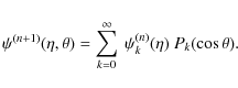
For completeness, we display the general solution of the <i>n</i>th iterative step:
<p></p>
<DIV ALIGN="CENTER">

<!-- MATH: \begin{equation}
\begin{array}{ll}
\psi^{(n+1)}(\eta, \theta)=& \Psi +\left[\int_{0}^{\eta}\eta'\hat\rho^{(n)}_{0}(\eta'){\rm d}\eta'-{1\over \eta}\int_{0}^{\eta} \eta'^2\hat\rho^{(n)}_{0}(\eta'){\rm d}\eta'
\right] \\
&-\sum_{k=2}^{\infty}{{P_k(\cos\theta)}\over{2k+1}}\left[\eta^k \int^{\infty}_{\eta} \eta'^{1-k}\hat\rho^{(n)}_{k}(\eta')d\eta'  \right.\\
&\left.+{1\over{\eta^{k+1}}}\int_{0}^{\eta}\eta'^{k+2}\hat\rho^ {(n)}_{k}(\eta'){\rm d}\eta' \right]
\end{array}
\end{equation} -->
<TABLE ALIGN="CENTER" WIDTH="100%">
<tbody><tr VALIGN="MIDDLE"><td ALIGN="CENTER" nowrap="nowrap"><IMG SRC="img194.png" ALT="\begin{displaymath}\begin{array}{ll}
\psi^{(n+1)}(\eta, \theta)=&amp; \Psi +\left[\i...
...{k+2}\hat\rho^ {(n)}_{k}(\eta'){\rm d}\eta' \right]
\end{array}\end{displaymath}" HEIGHT="111" WIDTH="353">
</td>
<td ALIGN="RIGHT" WIDTH="10">
(A.5)
</td>
</tr>
</table></div><br clear="all"><p></p>
where we have used the notation 
<!-- MATH: $\psi(0, \theta)=\Psi$ -->
<IMG SRC="img195.png" ALT="$\psi(0, \theta)=\Psi$" ALIGN="MIDDLE" BORDER="0" HEIGHT="26" WIDTH="68">.
The iteration can be stopped when the desired accuracy prescription is met, as for example when in the relevant domain 
<!-- MATH: $\mathcal{D}$ -->
<IMG SRC="img196.png" ALT="$\mathcal{D}$" ALIGN="MIDDLE" BORDER="0" HEIGHT="26" WIDTH="15">
we find that
<p></p>
<DIV ALIGN="CENTER">

<!-- MATH: \begin{equation}
\max_{(\xi,\zeta)\in\mathcal{D}}\left|{{\psi^{(n+1)}
-\psi^{(n)}}\over{\psi^{(n+1)}+\psi^{(n)}}}\right|<\epsilon .
\end{equation} -->
<TABLE ALIGN="CENTER" WIDTH="100%">
<tbody><tr VALIGN="MIDDLE"><td ALIGN="CENTER" nowrap="nowrap"><A NAME="erriter"></A><IMG SRC="img197.png" ALT="\begin{displaymath}\max_{(\xi,\zeta)\in\mathcal{D}}\left\vert{{\psi^{(n+1)}
-\psi^{(n)}}\over{\psi^{(n+1)}+\psi^{(n)}}}\right\vert&lt;\epsilon .
\end{displaymath}" HEIGHT="74" WIDTH="153">
</td>
<td ALIGN="RIGHT" WIDTH="10">
(A.6)
</td>
</tr>
</table></div><br clear="all"><p></p>
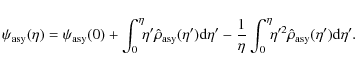
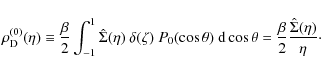
The dark matter gravitational potential is then separated into two
parts:
<p></p>
<DIV ALIGN="CENTER">

<!-- MATH: \begin{equation}
\psi_{\rm DM}\equiv \psi_{\rm asy}+\psi .
\end{equation} -->
<TABLE ALIGN="CENTER" WIDTH="100%">
<tbody><tr VALIGN="MIDDLE"><td ALIGN="CENTER" nowrap="nowrap"><A NAME="separation"></A><IMG SRC="img198.png" ALT="\begin{displaymath}\psi_{\rm DM}\equiv \psi_{\rm asy}+\psi .
\end{displaymath}" HEIGHT="49" WIDTH="101">
</td>
<td ALIGN="RIGHT" WIDTH="10">
(A.7)
</td>
</tr>
</table></div><br clear="all"><p></p>
The potential defined as 
<!-- MATH: $\psi_{\rm asy}$ -->
<IMG SRC="img199.png" ALT="$\psi_{\rm asy}$" ALIGN="MIDDLE" BORDER="0" HEIGHT="26" WIDTH="26">
obeys the Poisson
equation
<p></p>
<DIV ALIGN="CENTER">

<!-- MATH: \begin{equation}
\nabla^2\psi_{\rm asy}=\hat\rho_{\rm asy}
\end{equation} -->
<TABLE ALIGN="CENTER" WIDTH="100%">
<tbody><tr VALIGN="MIDDLE"><td ALIGN="CENTER" nowrap="nowrap"><A NAME="asysep"></A><IMG SRC="img200.png" ALT="\begin{displaymath}\nabla^2\psi_{\rm asy}=\hat\rho_{\rm asy}
\end{displaymath}" HEIGHT="53" WIDTH="84">
</td>
<td ALIGN="RIGHT" WIDTH="10">
(A.8)
</td>
</tr>
</table></div><br clear="all"><p></p>
and has the same asymptotic behavior as in
Eq.&nbsp;(<a href="/articles/aa/full_html/2010/11/aa14387-10/aa14387-10.html#boundary">20</a>). In this way the potential <IMG SRC="img201.png" ALT="$\psi$" ALIGN="MIDDLE" BORDER="0" HEIGHT="26" WIDTH="12">
converges
to zero at large radii and the related Poisson equation
<p></p>
<DIV ALIGN="CENTER">

<!-- MATH: \begin{equation}
\left({1\over\xi}{\partial\over{\partial\xi}}\xi{\partial\over {\partial\xi}}
+{\partial^2\over{\partial\zeta^2}}\right)\psi=-\alpha
\exp{\left[\psi_{\rm asy}+\psi_{\rm D}+\psi\right]}- \hat\rho_{\rm asy}
\end{equation} -->
<TABLE ALIGN="CENTER" WIDTH="100%">
<tbody><tr VALIGN="MIDDLE"><td ALIGN="CENTER" nowrap="nowrap"><A NAME="final"></A><IMG SRC="img202.png" ALT="\begin{displaymath}\left({1\over\xi}{\partial\over{\partial\xi}}\xi{\partial\ove...
...t[\psi_{\rm asy}+\psi_{\rm D}+\psi\right]}- \hat\rho_{\rm asy}
\end{displaymath}" HEIGHT="73" WIDTH="322">
</td>
<td ALIGN="RIGHT" WIDTH="10">
(A.9)
</td>
</tr>
</table></div><br clear="all"><p></p>
can be directly solved by the iterative multipole
expansion outlined previously.

<p>Obviously, there is an infinite number of pairs 
<!-- MATH: $(\hat\rho_{\rm asy}, \psi_ {\rm asy})$ -->
<IMG SRC="img203.png" ALT="$(\hat\rho_{\rm asy}, \psi_ {\rm asy})$" ALIGN="MIDDLE" BORDER="0" HEIGHT="26" WIDTH="62">
that meet the conditions of Eqs.&nbsp;(<a href="/articles/aa/full_html/2010/11/aa14387-10/aa14387-10.html#asysep">A.8</a>) and (<a href="/articles/aa/full_html/2010/11/aa14387-10/aa14387-10.html#boundary">20</a>). Therefore, the construction method proposed below just reflects one reasonable choice. We decided to take 
<!-- MATH: $\hat\rho_{\rm asy}$ -->
<IMG SRC="img204.png" ALT="$\hat\rho_{\rm asy}$" ALIGN="MIDDLE" BORDER="0" HEIGHT="26" WIDTH="23">
and 
<!-- MATH: $\psi_{\rm asy}$ -->
<IMG SRC="img199.png" ALT="$\psi_{\rm asy}$" ALIGN="MIDDLE" BORDER="0" HEIGHT="26" WIDTH="26">
with spherical symmetry, because the relevant asymptotic condition for 
<!-- MATH: $\psi_{\rm asy}$ -->
<IMG SRC="img199.png" ALT="$\psi_{\rm asy}$" ALIGN="MIDDLE" BORDER="0" HEIGHT="26" WIDTH="26">
is characterized by spherical symmetry and because the spherical Poisson equation admits a simple explicit solution:
<br></p><p></p>
<DIV ALIGN="CENTER">

<!-- MATH: \begin{equation}
\psi_{\rm asy}(\eta)=\psi_{\rm asy}(0)+\int_{0}^{\eta}\!\!\eta'\hat\rho_ {\rm asy}(\eta'){\rm d}\eta'-{1\over\eta}\int_{0}^{\eta}\!\!\eta'^2\hat\rho_{\rm asy} (\eta'){\rm d}\eta' .~
\end{equation} -->
<TABLE ALIGN="CENTER" WIDTH="100%">
<tbody><tr VALIGN="MIDDLE"><td ALIGN="CENTER" nowrap="nowrap"><A NAME="spherical"></A><IMG SRC="img205.png" ALT="\begin{displaymath}\psi_{\rm asy}(\eta)=\psi_{\rm asy}(0)+\int_{0}^{\eta}\!\!\et...
...{0}^{\eta}\!\!\eta'^2\hat\rho_{\rm asy} (\eta'){\rm d}\eta' .~
\end{displaymath}" HEIGHT="70" WIDTH="355">
</td>
<td ALIGN="RIGHT" WIDTH="10">
(A.10)
</td>
</tr>
</table></div><br clear="all"><p></p>
The precise choice of the form of the density 
<!-- MATH: $\hat\rho_ {\rm asy}$ -->
<IMG SRC="img204.png" ALT="$\hat\rho_{\rm asy}$" ALIGN="MIDDLE" BORDER="0" HEIGHT="26" WIDTH="23">
is guided by the goal of simplifying the following numerical procedure to solve Eq.&nbsp;(<a href="/articles/aa/full_html/2010/11/aa14387-10/aa14387-10.html#final">A.9</a>). Different choices of the density 
<!-- MATH: $\hat\rho_{\rm asy}$ -->
<IMG SRC="img204.png" ALT="$\hat\rho_{\rm asy}$" ALIGN="MIDDLE" BORDER="0" HEIGHT="26" WIDTH="23">
correspond to different shapes of the potential <IMG SRC="img206.png" ALT="$\phi$" ALIGN="MIDDLE" BORDER="0" HEIGHT="26" WIDTH="10">
for the same pair of free parameters 
<!-- MATH: $(\alpha, \beta)$ -->
<IMG SRC="img14.png" ALT="$ (\alpha , \beta )$" ALIGN="MIDDLE" BORDER="0" HEIGHT="26" WIDTH="33">.
The adopted practical recipe to construct the density 
<!-- MATH: $\hat\rho_ {\rm asy}$ -->
<IMG SRC="img204.png" ALT="$\hat\rho_{\rm asy}$" ALIGN="MIDDLE" BORDER="0" HEIGHT="26" WIDTH="23">
turns out to be useful and efficient.

<p>
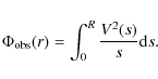
We start by defining what we call an ``observed'' pseudo-potential, constructed from the observed rotation curve:
<br></p><p></p>
<DIV ALIGN="CENTER">

<!-- MATH: \begin{equation}
\Phi_{\rm obs}(r)=\int_{0}^{R}{{V^2(s)}\over{s}}{\rm d}s.
\end{equation} -->
<TABLE ALIGN="CENTER" WIDTH="100%">
<tbody><tr VALIGN="MIDDLE"><td ALIGN="CENTER" nowrap="nowrap"><IMG SRC="img207.png" ALT="\begin{displaymath}\Phi_{\rm obs}(r)=\int_{0}^{R}{{V^2(s)}\over{s}}{\rm d}s.
\end{displaymath}" HEIGHT="73" WIDTH="145">
</td>
<td ALIGN="RIGHT" WIDTH="10">
(A.11)
</td>
</tr>
</table></div><br clear="all"><p></p>
<p>At large radii it has the asymptotic expression
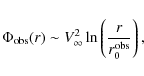
<br></p><p></p>
<DIV ALIGN="CENTER">

<!-- MATH: \begin{equation}
\Phi_{\rm obs}(r)\sim V^2_{\infty}\ln\left({r\over{r_0^{\rm obs}}}\right)  ,
\end{equation} -->
<TABLE ALIGN="CENTER" WIDTH="100%">
<tbody><tr VALIGN="MIDDLE"><td ALIGN="CENTER" nowrap="nowrap"><A NAME="apsiobs"></A><IMG SRC="img208.png" ALT="\begin{displaymath}\Phi_{\rm obs}(r)\sim V^2_{\infty}\ln\left({r\over{r_0^{\rm obs}}}\right) ,
\end{displaymath}" HEIGHT="76" WIDTH="144">
</td>
<td ALIGN="RIGHT" WIDTH="10">
(A.12)
</td>
</tr>
</table></div><br clear="all"><p></p>
<p>where the radius 
<!-- MATH: $r_0^{\rm obs}$ -->
<IMG SRC="img209.png" ALT="$r_0^{\rm obs}$" ALIGN="MIDDLE" BORDER="0" HEIGHT="30" WIDTH="24">
can be calculated from the precise form of the rotation curve. The behavior of Eq.&nbsp;(<a href="/articles/aa/full_html/2010/11/aa14387-10/aa14387-10.html#apsiobs">A.12</a>) naturally relates the potential 
<!-- MATH: $\Phi_{\rm obs}$ -->
<IMG SRC="img210.png" ALT="$\Phi_{\rm obs}$" ALIGN="MIDDLE" BORDER="0" HEIGHT="26" WIDTH="27">
(and its dimensionless counterpart 
<!-- MATH: $\psi_{\rm obs}$ -->
<IMG SRC="img211.png" ALT="$\psi_{\rm obs}$" ALIGN="MIDDLE" BORDER="0" HEIGHT="26" WIDTH="27">)
to a density distribution with isothermal functional shape:
<br></p><p></p>
<DIV ALIGN="CENTER">

<!-- MATH: \begin{equation}
{1\over{\eta^2}}{{\rm d}\over{{\rm d}\eta}}\eta^2{{\rm d}\over{{\rm d}\eta}}\psi_{\rm obs}(\eta) \sim-\alpha_{\rm obs}\exp\left[\psi_{\rm obs}(\eta)\right] ;\ \eta\gg1  .
\end{equation} -->
<TABLE ALIGN="CENTER" WIDTH="100%">
<tbody><tr VALIGN="MIDDLE"><td ALIGN="CENTER" nowrap="nowrap"><A NAME="alphaobs"></A><IMG SRC="img212.png" ALT="\begin{displaymath}{1\over{\eta^2}}{{\rm d}\over{{\rm d}\eta}}\eta^2{{\rm d}\ove...
...a_{\rm obs}\exp\left[\psi_{\rm obs}(\eta)\right] ;\ \eta\gg1 .
\end{displaymath}" HEIGHT="70" WIDTH="302">
</td>
<td ALIGN="RIGHT" WIDTH="10">
(A.13)
</td>
</tr>
</table></div><br clear="all"><p></p>
<p>As shown in Eq.&nbsp;(<a href="/articles/aa/full_html/2010/11/aa14387-10/aa14387-10.html#asycon">10</a>), the value of the constant 
<!-- MATH: $\alpha_{\rm obs}$ -->
<IMG SRC="img136.png" ALT="$\alpha_{\rm obs}$" ALIGN="MIDDLE" BORDER="0" HEIGHT="26" WIDTH="25">
is determined by the value of the radius 
<!-- MATH: $r_0^{\rm obs}$ -->
<IMG SRC="img209.png" ALT="$r_0^{\rm obs}$" ALIGN="MIDDLE" BORDER="0" HEIGHT="30" WIDTH="24">
only, and is thus fixed. Having made this points clear, we can define 
<!-- MATH: $\hat\rho_{\rm asy}$ -->
<IMG SRC="img204.png" ALT="$\hat\rho_{\rm asy}$" ALIGN="MIDDLE" BORDER="0" HEIGHT="26" WIDTH="23">
to be
<br></p><p></p>
<DIV ALIGN="CENTER">

<!-- MATH: \begin{equation}
\hat\rho_{\rm asy}(\eta)\equiv-\alpha_{\rm obs}\exp\left[\psi_{\rm obs}\left(\sqrt {\eta^2+\eta_{\rm c}^2}\right)\right]+\hat\rho_{\rm D}^{(0)}(\eta)  ,
\end{equation} -->
<TABLE ALIGN="CENTER" WIDTH="100%">
<tbody><tr VALIGN="MIDDLE"><td ALIGN="CENTER" nowrap="nowrap"><A NAME="dens1"></A><IMG SRC="img213.png" ALT="\begin{displaymath}\hat\rho_{\rm asy}(\eta)\equiv-\alpha_{\rm obs}\exp\left[\psi...
...2+\eta_{\rm c}^2}\right)\right]+\hat\rho_{\rm D}^{(0)}(\eta) ,
\end{displaymath}" HEIGHT="72" WIDTH="291">
</td>
<td ALIGN="RIGHT" WIDTH="10">
(A.14)
</td>
</tr>
</table></div><br clear="all"><p></p>
<p>where we have introduced a regularizing core structure with characteristic size <IMG SRC="img214.png" ALT="$\eta_c$" ALIGN="MIDDLE" BORDER="0" HEIGHT="26" WIDTH="15">
and subtracted the monopole term of the stellar density
<br></p><p></p>
<DIV ALIGN="CENTER">

<!-- MATH: \begin{equation}
\rho_{\rm D}^{(0)}(\eta)\equiv{\beta\over{2}}\int^{1}_{-1}\hat{\Sigma}(\eta) \ \delta(\zeta)\ P_0(\cos\theta)\ {\rm d}\cos\theta={\beta\over{2}}{{\hat {\Sigma}(\eta)}\over\eta} \cdot
\end{equation} -->
<TABLE ALIGN="CENTER" WIDTH="100%">
<tbody><tr VALIGN="MIDDLE"><td ALIGN="CENTER" nowrap="nowrap"><A NAME="monodisk"></A><IMG SRC="img215.png" ALT="\begin{displaymath}\rho_{\rm D}^{(0)}(\eta)\equiv{\beta\over{2}}\int^{1}_{-1}\ha...
...os\theta={\beta\over{2}}{{\hat {\Sigma}(\eta)}\over\eta} \cdot
\end{displaymath}" HEIGHT="73" WIDTH="321">
</td>
<td ALIGN="RIGHT" WIDTH="10">
(A.15)
</td>
</tr>
</table></div><br clear="all"><p></p>
With this density profile, from Eq.&nbsp;(<a href="/articles/aa/full_html/2010/11/aa14387-10/aa14387-10.html#spherical">A.10</a>) we calculate the gravitational potential 
<!-- MATH: $\psi_{\rm asy}$ -->
<IMG SRC="img199.png" ALT="$\psi_{\rm asy}$" ALIGN="MIDDLE" BORDER="0" HEIGHT="26" WIDTH="26">,
using the free constant 
<!-- MATH: $\psi_{\rm asy}(0)$ -->
<IMG SRC="img216.png" ALT="$ \psi_{\rm asy}(0)$" ALIGN="MIDDLE" BORDER="0" HEIGHT="26" WIDTH="41">
to make it meet exactly the asymptotic behavior required by Eq.&nbsp;(<a href="/articles/aa/full_html/2010/11/aa14387-10/aa14387-10.html#boundary">20</a>). The determination of the correct value of the constant 
<!-- MATH: $\psi_{\rm asy}(0)$ -->
<IMG SRC="img216.png" ALT="$ \psi_{\rm asy}(0)$" ALIGN="MIDDLE" BORDER="0" HEIGHT="26" WIDTH="41">
determines also the boundary condition to be used for Eq.&nbsp;(<a href="/articles/aa/full_html/2010/11/aa14387-10/aa14387-10.html#final">A.9</a>), which is set by the prescription:
<p></p>
<DIV ALIGN="CENTER">

<!-- MATH: \begin{equation}
\psi_{\rm T}(0,0)=\psi(0,0)+\psi_{\rm asy}(0)+\psi_{\rm D}(0,0)=0  .
\end{equation} -->
<TABLE ALIGN="CENTER" WIDTH="100%">
<tbody><tr VALIGN="MIDDLE"><td ALIGN="CENTER" nowrap="nowrap"><IMG SRC="img217.png" ALT="\begin{displaymath}\psi_{\rm T}(0,0)=\psi(0,0)+\psi_{\rm asy}(0)+\psi_{\rm D}(0,0)=0 .
\end{displaymath}" HEIGHT="50" WIDTH="265">
</td>
<td ALIGN="RIGHT" WIDTH="10">
(A.16)
</td>
</tr>
</table></div><br clear="all"><p></p>
<p></p><h3 class="sec2"><a name="SECTION000101000000000000000"></a>
A.1 The truncation of the angular expansion</h3>

<p>A code has been written to solve Eq.&nbsp;(<a href="/articles/aa/full_html/2010/11/aa14387-10/aa14387-10.html#final">A.9</a>)
through the technique described in the previous section. The code is
able to manage automatically the appropriate number of multipole terms
to meet a required accuracy (see Eq.&nbsp;(<a href="/articles/aa/full_html/2010/11/aa14387-10/aa14387-10.html#erriter">A.6</a>)). At each iterative step, the relevant number of multipole orders is calculated from the following prescription:
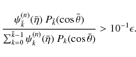
<br></p><p></p>
<DIV ALIGN="CENTER">

<!-- MATH: \begin{equation}
{{\psi_{\bar{k}}^{(n)}(\bar\eta)\ P_{\bar{k}}(\cos\bar\theta)}\over {\sum_{k=0}^{\bar{k}-1}\psi_{{k}}^{(n)}(\bar\eta)\ P_{{k}}(\cos\bar \theta)}}>10^{-1}\epsilon  .
\end{equation} -->
<TABLE ALIGN="CENTER" WIDTH="100%">
<tbody><tr VALIGN="MIDDLE"><td ALIGN="CENTER" nowrap="nowrap"><A NAME="nummult"></A><IMG SRC="img218.png" ALT="\begin{displaymath}{{\psi_{\bar{k}}^{(n)}(\bar\eta)\ P_{\bar{k}}(\cos\bar\theta)...
...^{(n)}(\bar\eta)\ P_{{k}}(\cos\bar \theta)}}&gt;10^{-1}\epsilon .
\end{displaymath}" HEIGHT="83" WIDTH="195">
</td>
<td ALIGN="RIGHT" WIDTH="10">
(A.17)
</td>
</tr>
</table></div><br clear="all"><p></p>
<p>In words, at the <i>n</i>th iteration step, the multipole term of order <IMG SRC="img219.png" ALT="$\bar k$" ALIGN="MIDDLE" BORDER="0" HEIGHT="30" WIDTH="10">
is retained in the expansion if its (relative) contribution to the gravitational potential 
<!-- MATH: $\psi^{(n)}$ -->
<IMG SRC="img191.png" ALT="$\psi^{(n)}$" ALIGN="MIDDLE" BORDER="0" HEIGHT="30" WIDTH="24">
(calculated with the previous <IMG SRC="img220.png" ALT="$\bar k -1$" ALIGN="MIDDLE" BORDER="0" HEIGHT="30" WIDTH="31">
multipole orders only) is comparable to the accuracy level <IMG SRC="img221.png" ALT="$\epsilon$" ALIGN="MIDDLE" BORDER="0" HEIGHT="26" WIDTH="10">
we want to meet. This comparison is made at the coordinates 
<!-- MATH: $(\bar\eta, \bar\theta)$ -->
<IMG SRC="img222.png" ALT="$(\bar\eta, \bar\theta)$" ALIGN="MIDDLE" BORDER="0" HEIGHT="29" WIDTH="31">,
chosen in the region where the deviation from spherical symmetry is strongest: 
<!-- MATH: $\bar\theta\approx\pi/2$ -->
<IMG SRC="img223.png" ALT="$\bar\theta\approx\pi/2$" ALIGN="MIDDLE" BORDER="0" HEIGHT="29" WIDTH="47">
and 
<!-- MATH: $\bar\eta\approx 1\div 2$ -->
<IMG SRC="img224.png" ALT="$\bar\eta\approx 1\div 2$" ALIGN="MIDDLE" BORDER="0" HEIGHT="26" WIDTH="55">.

</p><p>The models described in the paper are calculated with an accuracy prescription of 
<!-- MATH: $\epsilon=10^{-4}$ -->
<IMG SRC="img225.png" ALT="$\epsilon=10^{-4}$" ALIGN="MIDDLE" BORDER="0" HEIGHT="30" WIDTH="52">.
Obviously, the number of iterations required by such precision depends
on the gravitational importance of the stellar disk (which determines
the flattening of the halo). For values of the pair<!-- MATH: $(\alpha, \beta)$ -->
 <IMG SRC="img14.png" ALT="$ (\alpha , \beta )$" ALIGN="MIDDLE" BORDER="0" HEIGHT="26" WIDTH="33">
that represent an astrophysically realistic configuration (see Sect.&nbsp;<a href="/articles/aa/full_html/2010/11/aa14387-10/aa14387-10.html#Sect:Properties">4</a>), the number of required iterations is <IMG SRC="img226.png" ALT="$10\div20$" ALIGN="MIDDLE" BORDER="0" HEIGHT="26" WIDTH="46">,
with a number of multipole orders of <IMG SRC="img227.png" ALT="$12\div20$" ALIGN="MIDDLE" BORDER="0" HEIGHT="26" WIDTH="47">.

</p><p></p><h2 class="sec"><a name="SECTION000110000000000000000"></a><A NAME="wrongcorr"></A>Appendix B: Anomalous rotation curves 
</h2>

<p></p><div class="inset-old">
<table>
<tr><td><!-- init Label --><A NAME="ph"></A><!-- end Label--><A NAME="1544"></A><A NAME="figure1314" HREF="img228.png"><IMG SRC="Timg228.png" ALT="\begin{figure}
\par\includegraphics[width=8.7cm, angle=0]{14387fg22.eps} \end{figure}" HEIGHT="94" WIDTH="94"></A><!-- HTML Figure number: 22 -->
</td>
<td class="img-txt"><span class="bold">Figure B.1:</span><p>
Contours of the function <IMG SRC="img8.png" ALT="$\Xi $" align="bottom" BORDER="0" HEIGHT="14" WIDTH="12">
for the
       parametric decomposition (based on Eqs.&nbsp;(<a href="/articles/aa/full_html/2010/11/aa14387-10/aa14387-10.html#vd">1</a>, <a href="/articles/aa/full_html/2010/11/aa14387-10/aa14387-10.html#vdm">2</a>)) of the rotation curve defined by Eq.&nbsp;(<a href="/articles/aa/full_html/2010/11/aa14387-10/aa14387-10.html#paramprof">25</a>) with  
<!-- MATH: $\tau_{\rm f}=0.4$ -->
<IMG SRC="img15.png" ALT="$\tau _{\rm f}=0.4$" ALIGN="MIDDLE" BORDER="0" HEIGHT="26" WIDTH="49">.
</td>
</tr><tr><td colspan="2"><a href="http://dexter.edpsciences.org/applet.php?pdf_id=22&DOI=10.1051/0004-6361/201014387" target="DEXTER">Open with DEXTER</a></td></tr>

</table></div>  <br>
<p></p><div class="inset-old">
<table>
<tr><td><!-- init Label --><A NAME="nnph"></A><!-- end Label--><A NAME="1545"></A><A NAME="figure1324" HREF="img229.png"><IMG SRC="Timg229.png" ALT="\begin{figure}
\par\includegraphics[width=8.7cm, angle=0]{14387fg23.eps} \end{figure}" HEIGHT="93" WIDTH="96"></A><!-- HTML Figure number: 23 -->
</td>
<td class="img-txt"><span class="bold">Figure B.2:</span><p>
Contours of the function <IMG SRC="img8.png" ALT="$\Xi $" align="bottom" BORDER="0" HEIGHT="14" WIDTH="12">
for the self-consistent decomposition of the rotation curve defined by Eq.&nbsp;(<a href="/articles/aa/full_html/2010/11/aa14387-10/aa14387-10.html#paramprof">25</a>) with  
<!-- MATH: $\tau_{\rm f}=0.4$ -->
<IMG SRC="img15.png" ALT="$\tau _{\rm f}=0.4$" ALIGN="MIDDLE" BORDER="0" HEIGHT="26" WIDTH="49">.
</td>
</tr><tr><td colspan="2"><a href="http://dexter.edpsciences.org/applet.php?pdf_id=23&DOI=10.1051/0004-6361/201014387" target="DEXTER">Open with DEXTER</a></td></tr>

</table></div><div class="inset-old">
<table>
<tr><td><!-- init Label --><A NAME="hrc"></A><!-- end Label--><A NAME="1546"></A><A NAME="figure1331" HREF="img230.png"><IMG SRC="Timg230.png" ALT="\begin{figure}
\par\includegraphics[width=8.7cm, angle=0]{14387fg24.eps} \end{figure}" HEIGHT="67" WIDTH="97"></A><!-- HTML Figure number: 24 -->
</td>
<td class="img-txt"><span class="bold">Figure B.3:</span><p>
Disk-halo decomposition associated with
      the best self-consistent fit of the case 
<!-- MATH: $\tau_{\rm f}=0.4$ -->
<IMG SRC="img15.png" ALT="$\tau _{\rm f}=0.4$" ALIGN="MIDDLE" BORDER="0" HEIGHT="26" WIDTH="49">.
The coding is the same as in Fig.&nbsp;<a href="/articles/aa/full_html/2010/11/aa14387-10/aa14387-10.html#bfrc">12</a>.
</td>
</tr><tr><td colspan="2"><a href="http://dexter.edpsciences.org/applet.php?pdf_id=24&DOI=10.1051/0004-6361/201014387" target="DEXTER">Open with DEXTER</a></td></tr>

</table></div>
<p></p><div class="inset-old">
<table>
<tr><td><!-- init Label --><A NAME="pl"></A><!-- end Label--><A NAME="1547"></A><A NAME="figure1338" HREF="img231.png"><IMG SRC="Timg231.png" ALT="\begin{figure}
\par\includegraphics[width=8.7cm, angle=0]{14387fg25.eps} \end{figure}" HEIGHT="96" WIDTH="95"></A><!-- HTML Figure number: 25 -->
</td>
<td class="img-txt"><span class="bold">Figure B.4:</span><p>
Contours of the function <IMG SRC="img8.png" ALT="$\Xi $" align="bottom" BORDER="0" HEIGHT="14" WIDTH="12">
for the
       parametric decomposition (based on Eqs.&nbsp;(<a href="/articles/aa/full_html/2010/11/aa14387-10/aa14387-10.html#vd">1</a>), (<a href="/articles/aa/full_html/2010/11/aa14387-10/aa14387-10.html#vdm">2</a>)) of the rotation curve defined by Eq.&nbsp;(<a href="/articles/aa/full_html/2010/11/aa14387-10/aa14387-10.html#paramprof">25</a>) with  
<!-- MATH: $\tau_{s}=2.3$ -->
<IMG SRC="img16.png" ALT="$\tau _{s}=2.3$" ALIGN="MIDDLE" BORDER="0" HEIGHT="26" WIDTH="48">.
</td>
</tr><tr><td colspan="2"><a href="http://dexter.edpsciences.org/applet.php?pdf_id=25&DOI=10.1051/0004-6361/201014387" target="DEXTER">Open with DEXTER</a></td></tr>

</table></div><div class="inset-old">
<table>
<tr><td><!-- init Label --><A NAME="nnpl"></A><!-- end Label--><A NAME="1548"></A><A NAME="figure1347" HREF="img232.png"><IMG SRC="Timg232.png" ALT="\begin{figure}
\par\includegraphics[width=8.7cm, angle=0]{14387fg26.eps} \vspace*{1.5mm}
\end{figure}" HEIGHT="93" WIDTH="96"></A><!-- HTML Figure number: 26 -->
</td>
<td class="img-txt"><span class="bold">Figure B.5:</span><p>
Contours of the function <IMG SRC="img8.png" ALT="$\Xi $" align="bottom" BORDER="0" HEIGHT="14" WIDTH="12">
for the self-consistent decomposition of the rotation curve defined by Eq.&nbsp;(<a href="/articles/aa/full_html/2010/11/aa14387-10/aa14387-10.html#paramprof">25</a>) with  
<!-- MATH: $\tau_{\rm s}=2.3$ -->
<IMG SRC="img17.png" ALT="$\tau _{\rm s}=2.3$" ALIGN="MIDDLE" BORDER="0" HEIGHT="26" WIDTH="49">.
</td>
</tr><tr><td colspan="2"><a href="http://dexter.edpsciences.org/applet.php?pdf_id=26&DOI=10.1051/0004-6361/201014387" target="DEXTER">Open with DEXTER</a></td></tr>

</table></div>
<p></p><div class="inset-old">
<table>
<tr><td><!-- init Label --><A NAME="lrc"></A><!-- end Label--><A NAME="1549"></A><A NAME="figure1355" HREF="img233.png"><IMG SRC="Timg233.png" ALT="\begin{figure}
\par\includegraphics[width=8.7cm, angle=0]{14387fg27.eps} \end{figure}" HEIGHT="67" WIDTH="97"></A><!-- HTML Figure number: 27 -->
</td>
<td class="img-txt"><span class="bold">Figure B.6:</span><p>
Disk-halo decomposition associated with
      the best self-consistent fit of the case 
<!-- MATH: $\tau_{\rm s}=2.3$ -->
<IMG SRC="img17.png" ALT="$\tau _{\rm s}=2.3$" ALIGN="MIDDLE" BORDER="0" HEIGHT="26" WIDTH="49">.
The coding is the same as in Fig.&nbsp;<a href="/articles/aa/full_html/2010/11/aa14387-10/aa14387-10.html#bfrc">12</a>.
</td>
</tr><tr><td colspan="2"><a href="http://dexter.edpsciences.org/applet.php?pdf_id=27&DOI=10.1051/0004-6361/201014387" target="DEXTER">Open with DEXTER</a></td></tr>

</table></div>In this section we will analyze the case of rotation curves
with inner gradients that are significantly different from the one
identified by Eq.&nbsp;(<a href="/articles/aa/full_html/2010/11/aa14387-10/aa14387-10.html#corr">4</a>). These
rotation curves represent systems with a ``wrong tuning'' between the
disk and halo components, in the sense described in Sect.&nbsp;<a href="/articles/aa/full_html/2010/11/aa14387-10/aa14387-10.html#Sect:Conspiracy">2</a>. We adopt the same simple parametrization for the rotation curve shape as in Eq.&nbsp;(<a href="/articles/aa/full_html/2010/11/aa14387-10/aa14387-10.html#paramprof">25</a>) and consider two different values for the parameter <IMG SRC="img140.png" ALT="$\tau$" ALIGN="MIDDLE" BORDER="0" HEIGHT="26" WIDTH="9">,
taken to be significantly far from the value which that reproduces the correlation in Eq.&nbsp;(<a href="/articles/aa/full_html/2010/11/aa14387-10/aa14387-10.html#corr">4</a>). On the fast rising end, we take 
<!-- MATH: $\tau_{\rm f}=0.4$ -->
<IMG SRC="img15.png" ALT="$\tau _{\rm f}=0.4$" ALIGN="MIDDLE" BORDER="0" HEIGHT="26" WIDTH="49">
(i.e. 
<!-- MATH: $R_{\Omega}/h\approx0.44$ -->
<IMG SRC="img234.png" ALT="$R_{\Omega}/h\approx0.44$" ALIGN="MIDDLE" BORDER="0" HEIGHT="26" WIDTH="73">), while on the opposite side of a slowly rising rotation curve we take 
<!-- MATH: $\tau_{\rm s}=2.3$ -->
<IMG SRC="img17.png" ALT="$\tau _{\rm s}=2.3$" ALIGN="MIDDLE" BORDER="0" HEIGHT="26" WIDTH="49">
(i.e. 
<!-- MATH: $R_{\Omega}/h\approx2.53$ -->
<IMG SRC="img235.png" ALT="$R_{\Omega}/h\approx2.53$" ALIGN="MIDDLE" BORDER="0" HEIGHT="26" WIDTH="74">).
We apply the self-consistent and the parametric disk-halo decomposition
to these two anomalous rotation curves and refer to the same function <IMG SRC="img8.png" ALT="$\Xi $" align="bottom" BORDER="0" HEIGHT="14" WIDTH="12">
as in Eq.&nbsp;(<a href="/articles/aa/full_html/2010/11/aa14387-10/aa14387-10.html#deviat">29</a>) to quantify the quality of the fit. 

<p>The results for the fast rising rotation curve are shown in Figs.&nbsp;<a href="/articles/aa/full_html/2010/11/aa14387-10/aa14387-10.html#ph">B.1</a> and  <a href="/articles/aa/full_html/2010/11/aa14387-10/aa14387-10.html#nnph">B.2</a>.
In the parametric decomposition method we find again the bimodality of
the fit, as noted in the case of NGC&nbsp;3198. The self-consistent
method instead identifies a decomposition with an important stellar
disk; the fit for the rotation curve is illustrated in Fig.&nbsp;<a href="/articles/aa/full_html/2010/11/aa14387-10/aa14387-10.html#hrc">B.3</a>.

</p><p>The results for the slowly rising rotation curve are shown in Figs.&nbsp;<a href="/articles/aa/full_html/2010/11/aa14387-10/aa14387-10.html#pl">B.4</a> and  <a href="/articles/aa/full_html/2010/11/aa14387-10/aa14387-10.html#nnpl">B.5</a>.
The degeneracy pattern is clearly present in the parametric
decomposition, but in this case it is less marked with respect to the
cases studied earlier in this paper. Here, the parametric fit is
``pushed'' in the direction of an insignificant disk, because the
observed<!-- MATH: $R_{\Omega}$ -->
 <IMG SRC="img1.png" ALT="$R_{\Omega }$" ALIGN="MIDDLE" BORDER="0" HEIGHT="26" WIDTH="20">
is too small and can only be ascribed to a dominant dark matter halo.
On the other hand, the self-consistent decomposition appears to be able
to handle also this case (see Fig.&nbsp;<a href="/articles/aa/full_html/2010/11/aa14387-10/aa14387-10.html#lrc">B.6</a>).

</p><p>From the point of view of the quality of the fits, it is apparent that
both decomposition methods work best when fitting the case of<!-- MATH: $\tau\approx 1$ -->
 <IMG SRC="img236.png" ALT="$\tau\approx 1$" ALIGN="MIDDLE" BORDER="0" HEIGHT="26" WIDTH="33">,
that is for a rotation curve that follows the empirical correlation illustrated in Fig.&nbsp;<a href="/articles/aa/full_html/2010/11/aa14387-10/aa14387-10.html#corrfig">1</a>. This is the aspect of conspiracy that was introduced and described in Sect.&nbsp;<a href="/articles/aa/full_html/2010/11/aa14387-10/aa14387-10.html#empiric">2.1</a>. In this case, the values of the function <IMG SRC="img8.png" ALT="$\Xi $" align="bottom" BORDER="0" HEIGHT="14" WIDTH="12">
corresponding to the best-fitting 
<!-- MATH: $(\alpha,~ \beta)$ -->
<IMG SRC="img27.png" ALT="$(\alpha,~\beta)$" ALIGN="MIDDLE" BORDER="0" HEIGHT="26" WIDTH="38">
pairs are the smallest. In particular, Fig.&nbsp;<a href="/articles/aa/full_html/2010/11/aa14387-10/aa14387-10.html#hrc">B.3</a>
shows that the case of a fast rising rotation curve cannot be properly
described without including a central concentrated mass component, such
as a bulge; the value of the residuals <IMG SRC="img8.png" ALT="$\Xi $" align="bottom" BORDER="0" HEIGHT="14" WIDTH="12">
in correspondence of the best-fit (see Fig.&nbsp;<a href="/articles/aa/full_html/2010/11/aa14387-10/aa14387-10.html#nnph">B.2</a>) is considerably higher if compared for example to the good fit of Fig.&nbsp;<a href="/articles/aa/full_html/2010/11/aa14387-10/aa14387-10.html#bfrc">12</a>.
Similarly, for the opposite case of a slowly rising rotation curve, it
is the parametric model which is quite unable to account for such a
shape of the rotation velocity, with a similar high value for the
best-fit residuals (see Fig.&nbsp;<a href="/articles/aa/full_html/2010/11/aa14387-10/aa14387-10.html#pl">B.4</a>). 

</p><p></p>
</div></body></html>