| Issue |
A&A
Volume 519, September 2010
|
|
|---|---|---|
| Article Number | A75 | |
| Number of page(s) | 16 | |
| Section | Planets and planetary systems | |
| DOI | https://doi.org/10.1051/0004-6361/201014281 | |
| Published online | 15 September 2010 | |
Online Material
Appendix A: Solution of the Duhamel-Neumann equation
We outline the main steps needed to solve the Duhamel-Neumann
equation in Eq. (18) for our work. The temperature
field, which produces the thermal stresses, is assumed to have a
linearized form
![]() where
where ![]() is given
by Eq. (9).
The uniqueness of the solution arises from (i) the regularity in the
whole volume; and (ii) matching the free boundary conditions
(given by Eq. (19)) at the surface r = R.
is given
by Eq. (9).
The uniqueness of the solution arises from (i) the regularity in the
whole volume; and (ii) matching the free boundary conditions
(given by Eq. (19)) at the surface r = R.
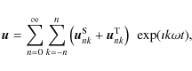
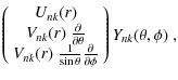
There are different ways in which we can decompose the
displacement vector ![]() into spherical-harmonics-type
expansion (see, e.g., Thorne 1980, for an insightful review).
Here we use a decomposition into spheroidal and toroidal components traditionally used in
geophysical analyses (e.g., Kaula 1968; Bullen 1975). With this
approach, related to what Thorne (1980) calls pure-spin vector
harmonics, we have
into spherical-harmonics-type
expansion (see, e.g., Thorne 1980, for an insightful review).
Here we use a decomposition into spheroidal and toroidal components traditionally used in
geophysical analyses (e.g., Kaula 1968; Bullen 1975). With this
approach, related to what Thorne (1980) calls pure-spin vector
harmonics, we have
with
The first component in Eq. (A.1),
The spheroidal character of our source (temperature) term the
Duhamel-Neumann equation implies two simplifications. First, the
toroidal part of the displacement vector becomes negligible and we
have Wnk=0. Second, we can restrict the summation over
degrees n in Eq. (A.1) to the dipole and higher-order
terms only, ignoring the monopole n=0. This is because the
monopole part would correspond to purely radial temperature field,
such as has been considered, for instance, in the previous works
on our topic (e.g., Tambovtseva & Shestakova 1999; Shestakova & Tambovtseva 1997; Kuehrt 1984).
Our temperature representation
![]() does not
contain a non-trivial, purely radial profile
does not
contain a non-trivial, purely radial profile![]() and the only viable free monopole term must have
U00=W00=0to match the boundary conditions. Finally, we note that we also
anticipated the Fourier-development structure in Eq. (A.1)
as it follows from the source (
and the only viable free monopole term must have
U00=W00=0to match the boundary conditions. Finally, we note that we also
anticipated the Fourier-development structure in Eq. (A.1)
as it follows from the source (![]() development).
development).
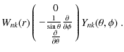
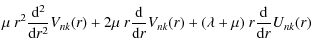
Substituting the spheroidal-vector representation of ![]() into
the Duhamel-Neumann Eq. (18) we obtain the
following system of equations for the radial profile of the
amplitude functions Unk(r) and Vnk(r) (
into
the Duhamel-Neumann Eq. (18) we obtain the
following system of equations for the radial profile of the
amplitude functions Unk(r) and Vnk(r) (![]() ):
):
and
Here we found it useful to separate the r- and t-dependences
of the
tnk(r,t) amplitudes of the ![]() development in
Eq. (9) and introduce pure radial parts
Tnk(r) such that
development in
Eq. (9) and introduce pure radial parts
Tnk(r) such that
![]() .
These represent source terms in Eqs. (A.4) and (A.5).
.
These represent source terms in Eqs. (A.4) and (A.5).
While the solution of Unk(r) and Vnk(r) is coupled by means of Eqs. (A.4) and (A.5), the fundamental implication of the Duhamel-Neumann equation linearity is that amplitude terms of different degrees and orders in the spherical harmonics development as well as the different Fourier modes are not mixed and can be solved separately.
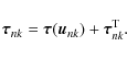
Once we obtain Unk(r) and Vnk(r), we can readily compute
components of the corresponding stress tensor
![]() arising from the displacement vector
field by using the Hook's law in Eq. (16).
Given its linearity, we thus again have
arising from the displacement vector
field by using the Hook's law in Eq. (16).
Given its linearity, we thus again have
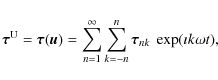
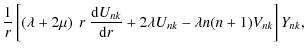
where
![$\displaystyle \frac{\mu}{r}\left[ U_{nk}+r~\frac{{\rm d} V_{nk}}{{\rm d} r}
-V_{nk} \right]\frac{\partial}{\partial\theta}Y_{nk},$](/articles/aa/olm/2010/11/aa14281-10/img261.png)
![$\displaystyle \frac{\mu}{r}\left[ U_{nk}+r~\frac{{\rm d} V_{nk}}{{\rm d} r}
-V_{nk} \right]\frac{\imath k}{\sin\theta} Y_{nk}\; ,$](/articles/aa/olm/2010/11/aa14281-10/img263.png)
![$\displaystyle \lambda~r~\frac{{\rm d} U_{nk}}{{\rm d} r}\Bigr]Y_{nk}+2\mu\frac{V_{nk}}{r}
\frac{\partial}{\partial\theta}Y_{nk},$](/articles/aa/olm/2010/11/aa14281-10/img265.png)
![$\displaystyle \lambda~r~\frac{{\rm d} U_{nk}}{{\rm d} r}\Bigr]Y_{nk}
-2\mu~\frac{V_{nk}}{r}\frac{\partial^2 }{\partial \theta^2}Y_{nk},$](/articles/aa/olm/2010/11/aa14281-10/img267.png)
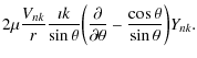
The partial derivatives of the spherical functions Ynk are computed using
| |
= | ||
| (A.13) | |||
| = | ![$\displaystyle \left[ \frac{k^2}{\sin^2\theta}-n(n+1) \right]
Y_{nk}-\frac{\cos\theta}{\sin\theta}\frac{\partial }{\partial \theta}Y_{nk}.$](/articles/aa/olm/2010/11/aa14281-10/img274.png)
|
(A.14) |
Equations (A.7) to (A.12) yield components of the stress tensor that explicitly depend on the displacement vector
Because of the linearity of the Duhamel-Neumann equation, a general solution is expressed in terms of a linear superposition of (i) a solution of the homogeneous system; and (ii) a particular solution of the inhomogeneous system. The next two sections discuss the two cases separately.
A.1 Solution of the homogeneous Duhamel-Neumann equation
Equations (A.4) and (A.5)
with zero right-hand sides represent the homogeneous
Duhamel-Neumann equation broken into parts corresponding to the
individual spheroidal modes. Its solution is quite complicated,
but may be significantly simplified in our case. This is because
for the range of material parameters, sizes and rotation
frequencies that apply for meteoroids we always have![]()
![]() .
With these we may
neglect the troublesome term
.
With these we may
neglect the troublesome term
![]() in
Eqs. (A.4) and (A.5). A major implication
of this is then that the system of solutions of the homogeneous
Duhamel-Neumann equation become degenerate in the k (order)
index of the spherical-harmonics representation.
in
Eqs. (A.4) and (A.5). A major implication
of this is then that the system of solutions of the homogeneous
Duhamel-Neumann equation become degenerate in the k (order)
index of the spherical-harmonics representation.
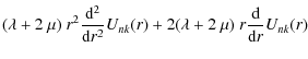
Adopting the aforementioned approximation, the homogeneous system
of Eqs. (A.4) and (A.5) now has a form of
Euler equations. As such, it has a fundamental system of power-law
solutions
Uink=Qi rmi and
Vink = rmi with
![]() ,
real-valued exponents mi and amplitudes Qi.
After a straightforward algebra, we obtain
,
real-valued exponents mi and amplitudes Qi.
After a straightforward algebra, we obtain
| U1nk(r) | = | (A.15) | |
| V1nk(r) | = | rn+1, | (A.16) |
| U2nk(r) | = | (A.17) | |
| U3nk(r) | = | (A.18) | |
| U4nk(r) | = | (A.19) | |
| V4nk(r) | = | r-n. | (A.20) |
The last two modes, 3 and 4, diverge at the center r=0 and therefore must be excluded. We are thus left with the first two modes, 1 and 2, that produce the spheroidal modes
A.2 Particular solution of the Duhamel-Neumann equation
We next find a particular solution of the
inhomogeneous Duhamel-Neumann equation with the thermal source
![]() .
We divide this task into a discussion of the
stationary case (k=0) and time-dependent case (
.
We divide this task into a discussion of the
stationary case (k=0) and time-dependent case (![]() ). In
both cases, we again use the approximation of neglecting the
). In
both cases, we again use the approximation of neglecting the
![]() terms in Eqs. (A.4) and (A.5).
terms in Eqs. (A.4) and (A.5).
A.2.1 Time-independent part
The stationary temperature field is given by
![]() (Eqs. (9) and (10)) and thus
(Eqs. (9) and (10)) and thus
![]() .
We again search the fundamental
system of solutions in a power-law form
.
We again search the fundamental
system of solutions in a power-law form
![]() and
and
![]() with some real-valued exponents
with some real-valued exponents
![]() and
amplitudes
and
amplitudes
![]() .
After a brief algebraic
derivation, we obtain
.
After a brief algebraic
derivation, we obtain
| |
= | (A.21) | |
| = | (A.22) |
We note that this mode has the same radial profile as the
A.2.2 Time-dependent part
The time-dependent temperature field is given by
![]() with
with ![]() (Eqs. (9) and (11)) and thus
(Eqs. (9) and (11)) and thus
![]() .
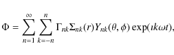
We assume that the particular
solution has a form
.
We assume that the particular
solution has a form
![]() .
Substituting
this ansätz to the Duhamel-Neumann equation
Eq. (18), we obtain
.
Substituting
this ansätz to the Duhamel-Neumann equation
Eq. (18), we obtain
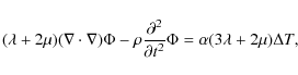
where we have suitably assumed that the arbitrary constant on the right-hand side canceled the monopole (constant) temperature part. This is an inhomogeneous wave equation on a sphere that, however, takes a simple form because of the spherical-harmonic and Fourier structure of the source term
we obtain
and
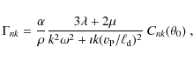
where
| |
= | (A.27) | |
| = | (A.28) |
The corresponding stress tensor is expressed by Eqs. (58)-(63).
A.3 Complete expression of the thermal stress tensor
The complete solution of the Duhamel-Neumann
equation is a linear combination of the free-spheroidal modes
![]() and
and
![]() from Sect. A.1
and the particular mode
from Sect. A.1
and the particular mode
![]() from Sect. A.2.
In the individual spherical harmonics modes, we have
from Sect. A.2.
In the individual spherical harmonics modes, we have
![]() ,
where Q1nk and Q2nk are
some coefficients. We have to choose them to satisfy the surface
boundary condition (19), namely
,
where Q1nk and Q2nk are
some coefficients. We have to choose them to satisfy the surface
boundary condition (19), namely
![]() at r=R. Here the total stress tensor is given by
at r=R. Here the total stress tensor is given by

or again in the spherical harmonics modes
The truly active and independent conditions are
We were able to carry out all necessary algedraic manipulations and obtain a close form of the resulting formulae for the case of the stationary (zonal, k=0) part of the stress field. These are given in Eqs. (36)-(39) (Sect. 3.1.1). In the case of the time-dependent part of the stress field, the algebra is more involved and we could not reach as simple and compact results as for the time-independent part. We thus confine ourselves to provide formulae for the stress-tensor components of the individual components and those for the integration constants Q1nk and Q2nk(Sect. 3.1.2).
Current usage metrics show cumulative count of Article Views (full-text article views including HTML views, PDF and ePub downloads, according to the available data) and Abstracts Views on Vision4Press platform.
Data correspond to usage on the plateform after 2015. The current usage metrics is available 48-96 hours after online publication and is updated daily on week days.
Initial download of the metrics may take a while.