Online Material
Appendix A:  surfaces for RADEX fits
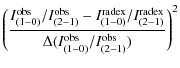
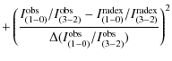
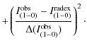
Figures A.1-A.8 show the ![]() surfaces from the
non-LTE analysis of the line integrated intensity ratios for each of the
positions studied. The
surfaces from the
non-LTE analysis of the line integrated intensity ratios for each of the
positions studied. The ![]() has been calculated using
Eq. (A.1), where
has been calculated using
Eq. (A.1), where
![]() is the
observed integrated intensity of the transition between
is the
observed integrated intensity of the transition between
![]() and
and
![]() ,
,
![]() (x) is the uncertainty on the quantity x and, finally,
(x) is the uncertainty on the quantity x and, finally,
![]() is the integrated intensity for each
transition as modelled by RADEX, for each combination of temperature and gas
column density
is the integrated intensity for each
transition as modelled by RADEX, for each combination of temperature and gas
column density
For each case, the ![]() is plotted as a function of the RADEX output
temperature and gas column density. Given the use of 3 quantities in the fit,
we consider
is plotted as a function of the RADEX output
temperature and gas column density. Given the use of 3 quantities in the fit,
we consider
![]() ,
i.e. the reduced-
,
i.e. the reduced-
![]() a good fit. All
figures have contours at
a good fit. All
figures have contours at
![]() ,
2 and 3 with the exception of ND
(Fig. A.4) and SD (Fig. A.8).
,
2 and 3 with the exception of ND
(Fig. A.4) and SD (Fig. A.8).
![\begin{figure}
\par\includegraphics[scale=.37,angle=-90]{13919fga1.eps}
\end{figure}](img90.png)
|
Figure A.1:
|
| Open with DEXTER | |
![\begin{figure}
\par\includegraphics[scale=.37,angle=-90]{13919fga2.eps}
\end{figure}](img91.png)
|
Figure A.2:
|
| Open with DEXTER | |
![\begin{figure}
\par\includegraphics[scale=.37,angle=-90]{13919fga3.eps}
\end{figure}](img92.png)
|
Figure A.3:
|
| Open with DEXTER | |
![\begin{figure}
\par\includegraphics[scale=.37,angle=-90]{13919fga4.eps}
\end{figure}](img93.png)
|
Figure A.4:
|
| Open with DEXTER | |
![\begin{figure}
\mbox{\includegraphics[scale=.37,angle=-90]{13919fga5a.eps} \h...
...egraphics[scale=.37,angle=-90]{13919fga5b.eps} }
\hfill
\hfill
\end{figure}](img94.png)
|
Figure A.5:
|
| Open with DEXTER | |
![\begin{figure}
\mbox{\includegraphics[scale=.37,angle=-90]{13919fga6a.eps} \h...
...udegraphics[scale=.37,angle=-90]{13919fga6b.eps} }
\hfill
\hfill\end{figure}](img95.png)
|
Figure A.6:
|
| Open with DEXTER | |
![\begin{figure}
\mbox{\includegraphics[scale=.37,angle=-90]{13919fga7a.eps} \h...
...degraphics[scale=.37,angle=-90]{13919fga7b.eps} }
\hfill
\hfill
\end{figure}](img96.png)
|
Figure A.7:
|
| Open with DEXTER | |
![\begin{figure}
\mbox{\includegraphics[scale=.38,angle=-90]{13919fga8a.eps} \h...
...degraphics[scale=.38,angle=-90]{13919fga8b.eps} }
\hfill
\hfill\end{figure}](img97.png)
|
Figure A.8:
|
| Open with DEXTER | |
Appendix B: C18O intensities and abundances
Table B.1 presents the best fit integrated intensities from the non-LTE (RADEX) modelling (Appendix A) , together with the observed values, and the implied C18O abundances.
Table B.1: Modelled integrated intensities and resulting abundances.
For positions ND, SB, SC and SD, the H2 column densities derived from the dust and used to estimate the abundance of C18O were calculated using a dust temperature of 10 K. Assuming a temperature of 15 K for all 4 positions (ND, SB, SC and SD) would reduce the H2 column densities by a factor of 2.1, representing an equivalent rise of the fractal abundance of C18O by the same amount.
The derived C18O fractional abundance (which is averaged along the line
of sight) implies a depletion of C18O of between a factor of 1.4 (for NC)
and 4.3 (for SC), with an average of 2.5 compared to the abundance of
![]() in dark clouds (Frerking et al. 1982). Given that the
ratio between C17O and C18O has shown these two species to be
optically thin, with an intensity ratio of
in dark clouds (Frerking et al. 1982). Given that the
ratio between C17O and C18O has shown these two species to be
optically thin, with an intensity ratio of ![]() 3.5, a factor 2.5 depletion
of C18O implies the same depletion factor for C17O.
3.5, a factor 2.5 depletion
of C18O implies the same depletion factor for C17O.