| Issue |
A&A
Volume 505, Number 2, October II 2009
|
|
|---|---|---|
| Page(s) | 695 - 706 | |
| Section | Stellar structure and evolution | |
| DOI | https://doi.org/10.1051/0004-6361/200810972 | |
| Published online | 24 July 2009 | |
Online Material
Appendix A: (Circum)Stellar parameters from SED fits
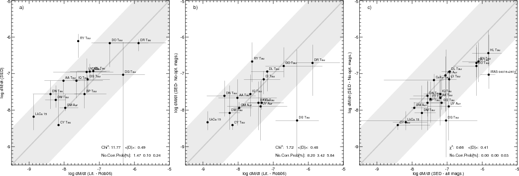 |
Figure A.1:
Comparison between mass accretion rates from the literature
and those derived from SED fits for the sample of T-Tauri stars
considered in Robitaille et al. (2006). SED fits and determination of parameter
ranges were performed as for the |
| Open with DEXTER | |
In this appendix, we describe how we constrained some stellar and circumstellar parameters of the objects in our sample by comparing their SEDs with the theoretical models of Robitaille et al. (2006). These consist of a grid of 200 000 model SEDs that include contributions from the central star, the circumstellar disk, and the envelope, parametrized with 14 parameters. The models that best approximate the observed SEDs were found with the aid of the Web-based tool presented by Robitaille et al. (2007). As stated by Robitaille et al. (2007), and in accord with basic principles, this method does not allow the simultaneous determination of all 14 physical parameters, since the SEDs are often defined by less than 14 independent fluxes. However, depending on the available fluxes, some of the parameters can be constrained more narrowly than others. We are interested here, in particular, in obtaining the range of values compatible with the observed SEDs for: i) the extinction toward our objects; ii) their disk accretion rates.
A.1 The method and its validation
Our procedure follows closely that of Robitaille et al. (2007): from the Web
interface we obtain, for each object, a list of the 1000 models that
best approximate the observed SEDs, i.e. those with the smallest ![]() .
Our ``best guess'' parameter values and associated
confidence intervals are then derived by selecting a set of statistically reasonable models and computing the median and the
.
Our ``best guess'' parameter values and associated
confidence intervals are then derived by selecting a set of statistically reasonable models and computing the median and the
![]()
![]() quantiles of the parameter values for these models. The
statistically reasonable models were defined as those with reduced
quantiles of the parameter values for these models. The
statistically reasonable models were defined as those with reduced
![]() ,
where
,
where
![]() refers to
the best fit model, or if this condition results in less than 10 models, the 10 models with smallest
refers to
the best fit model, or if this condition results in less than 10 models, the 10 models with smallest ![]() .
Note that, because
the uncertainties on the observed SEDs are not well defined (see
below), and the parameter space is sampled only discretely by the
adopted grid of models, the statistical significance of the thus
derived confidence intervals cannot be easily assessed.
.
Note that, because
the uncertainties on the observed SEDs are not well defined (see
below), and the parameter space is sampled only discretely by the
adopted grid of models, the statistical significance of the thus
derived confidence intervals cannot be easily assessed.
A similar method![]() was tested by Robitaille et al. (2007) by considering a sample of
Taurus-Auriga objects for which stellar and circumstellar parameters
had been derived independently in the literature and comparing these
parameters with those obtained from fitting the SEDs, defined from the
optical to millimeter wavelengths. In the case of our heavily absorbed
was tested by Robitaille et al. (2007) by considering a sample of
Taurus-Auriga objects for which stellar and circumstellar parameters
had been derived independently in the literature and comparing these
parameters with those obtained from fitting the SEDs, defined from the
optical to millimeter wavelengths. In the case of our heavily absorbed
![]() Ophiuchi YSOs, the SEDs lack, with the exception of one star,
data in the optical bands, i.e. those more directly affected by the
accretion-shock emission. In order to test our ability to constrain
the accretion rates in the absence of optical information, we repeated
the SED fits of the Taurus-Auriga stars of Robitaille et al. (2007), using the
same datapoints to define the SEDs, and both including and excluding
the optical magnitudes. The results are shown in
Fig. A.1. Panel a), analogous to Fig. 2b in
Robitaille et al. (2007), compares the accretion rates derived from the SED fits,
including optical data, with independent values from the literature.
Panel b) compares the results of the SED fits without the optical
magnitudes with the literature data. The agreement between the two
quantities is acceptable and may actually be considered better than in
the former panel: the reduced
Ophiuchi YSOs, the SEDs lack, with the exception of one star,
data in the optical bands, i.e. those more directly affected by the
accretion-shock emission. In order to test our ability to constrain
the accretion rates in the absence of optical information, we repeated
the SED fits of the Taurus-Auriga stars of Robitaille et al. (2007), using the
same datapoints to define the SEDs, and both including and excluding
the optical magnitudes. The results are shown in
Fig. A.1. Panel a), analogous to Fig. 2b in
Robitaille et al. (2007), compares the accretion rates derived from the SED fits,
including optical data, with independent values from the literature.
Panel b) compares the results of the SED fits without the optical
magnitudes with the literature data. The agreement between the two
quantities is acceptable and may actually be considered better than in
the former panel: the reduced ![]() ,
computed from the identity
relation considering only uncertainties on
,
computed from the identity
relation considering only uncertainties on
![]() ,
is indeed
reduced from
,
is indeed
reduced from ![]() 12 to 1.7. This can in part be attributed to the
increased error bars; note, however, that the average of the unsigned
differences, abs(
12 to 1.7. This can in part be attributed to the
increased error bars; note, however, that the average of the unsigned
differences, abs(
![]() ), is almost
unchanged, 0.49 dex for panel a) and 0.48 dex for panel b).
Panel c) compares the
), is almost
unchanged, 0.49 dex for panel a) and 0.48 dex for panel b).
Panel c) compares the ![]() from the SED fits with and without
optical magnitudes, showing that the two sets of values agree within
uncertainties. We conclude that the SEDs defined from IR to
millimeter wavelengths are indeed sensitive to the accretion rate, at
least in the
from the SED fits with and without
optical magnitudes, showing that the two sets of values agree within
uncertainties. We conclude that the SEDs defined from IR to
millimeter wavelengths are indeed sensitive to the accretion rate, at
least in the ![]() range covered by the Taurus-Auriga sample:
log
range covered by the Taurus-Auriga sample:
log
![]() .
.
This is due to the effect of viscous heating affecting the disk
thermal structure. To exemplify this effect we plot in
Fig. A.2, as a function of accretion rate, the ratio
between the IRAC 3 band and the J-band flux, for the Robitaille et al. (2006)
models for stars with mass between 0.7 and 1.3 ![]() ,
age between 1 and 2 Myr (implying little or no circumstellar envelope), and low
disk inclination with respect to the line of sight (
,
age between 1 and 2 Myr (implying little or no circumstellar envelope), and low
disk inclination with respect to the line of sight (
![]() ).
We plot with different symbols models with disk inner radii in
different ranges, since the inner hole affects the flux at the IRAC 3
wavelength (5.8
).
We plot with different symbols models with disk inner radii in
different ranges, since the inner hole affects the flux at the IRAC 3
wavelength (5.8 ![]() m). A relation between the two quantities is
seen for models with moderate inner disk holes, apparently
characterized by different regimes in three different
m). A relation between the two quantities is
seen for models with moderate inner disk holes, apparently
characterized by different regimes in three different ![]() ranges:
ranges:
![]() ,
,
![]() ,
and
,
and
![]() .
The factor of
.
The factor of ![]() 2 scatter
around this relation may likely be attributed to model variations
within the specified parameter ranges and to the several other
unconstrained model parameters. Similar and even more pronounced
trends are apparent in analogous plots using fluxes in longer
wavelength IRAC and MIPS bands, with the expected difference that at
the longer wavelengths, emitted farther out in the disk, the size of
the inner hole has a much smaller effect. The three regimes in
Fig. A.2 can be understood as follows: i) for
large accretion rates,
2 scatter
around this relation may likely be attributed to model variations
within the specified parameter ranges and to the several other
unconstrained model parameters. Similar and even more pronounced
trends are apparent in analogous plots using fluxes in longer
wavelength IRAC and MIPS bands, with the expected difference that at
the longer wavelengths, emitted farther out in the disk, the size of
the inner hole has a much smaller effect. The three regimes in
Fig. A.2 can be understood as follows: i) for
large accretion rates,
![]() ,
the flux in
the IRAC band, emitted by the inner disk (R<1 AU), is significantly
affected by viscous accretion (D'Alessio et al. 1998,1999); ii) for
,
the flux in
the IRAC band, emitted by the inner disk (R<1 AU), is significantly
affected by viscous accretion (D'Alessio et al. 1998,1999); ii) for
![]() disk heating is
dominated by the stellar photospheric emission and, consequently, no
relation between the IRAC flux and
disk heating is
dominated by the stellar photospheric emission and, consequently, no
relation between the IRAC flux and ![]() is observed; iii) for
is observed; iii) for
![]() we again observe a direct
relation between the IRAC 3 flux and
we again observe a direct
relation between the IRAC 3 flux and ![]() ,
which we attribute to
the fact that these low accretion rates correspond, in the
Robitaille et al. (2006) model grid, to very low disk masses (
,
which we attribute to
the fact that these low accretion rates correspond, in the
Robitaille et al. (2006) model grid, to very low disk masses (
![]() for the
for the ![]() 1 solar mass stars
plotted in Fig. A.2). Since, in the model grid, disk
mass and accretion are directly correlated and such low mass disks are
optically thin (Robitaille et al. 2006), lower accretion rates imply lower disk
mass and lower emission in the IRAC band. The IRAC 3 flux vs.
1 solar mass stars
plotted in Fig. A.2). Since, in the model grid, disk
mass and accretion are directly correlated and such low mass disks are
optically thin (Robitaille et al. 2006), lower accretion rates imply lower disk
mass and lower emission in the IRAC band. The IRAC 3 flux vs.
![]() correlation in this regime does not therefore imply that
that the mid-IR SED carries direct information on disk
accretion.
correlation in this regime does not therefore imply that
that the mid-IR SED carries direct information on disk
accretion.
As a result of this discussion, in the derivation of accretion rates
for our ![]() Ophiuchi sample from the SED fits, we decided not to
use values below
Ophiuchi sample from the SED fits, we decided not to
use values below
![]() yr-1. In such cases we
instead conservatively assigned upper limits to
yr-1. In such cases we
instead conservatively assigned upper limits to ![]() equal to the
maximum between
equal to the
maximum between
![]() yr-1 and the upper end of
the
yr-1 and the upper end of
the ![]() confidence interval (see above).
confidence interval (see above).
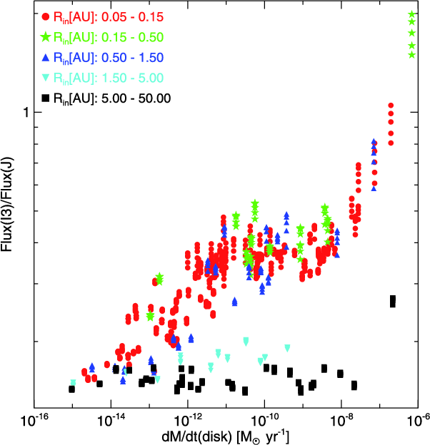 |
Figure A.2:
Scatter plot of the ratio between the flux in the IRAC 1
band over that in J, as a function of
disk accretion rate, according to the Robitaille et al. (2006) models for a solar
mass stars. Each point corresponds to one of the Robitaille et al. (2006) models
satisfying the following conditions: mass of the central object
between 0.7 and 1.3 |
| Open with DEXTER | |
A.2 The  Ophiuchi sample
We collected photometric measurements and uncertainties (when
available) for our ![]() Ophiuchi sample from several sources: J,
H, and
Ophiuchi sample from several sources: J,
H, and ![]() magnitudes (or upper limits) were taken for almost all
objects from 2 MASS
magnitudes (or upper limits) were taken for almost all
objects from 2 MASS![]() ; Spitzer IRAC (bands 1-4) and MIPS (bands 1 &
2) photometry was collected from the c2d database
; Spitzer IRAC (bands 1-4) and MIPS (bands 1 &
2) photometry was collected from the c2d database![]() (Evans et al. 2003); 1.2 mm
fluxes were collected from Stanke et al. (2006) and 1.3 mm fluxes from
Andre & Montmerle (1994)
(Evans et al. 2003); 1.2 mm
fluxes were collected from Stanke et al. (2006) and 1.3 mm fluxes from
Andre & Montmerle (1994)![]() . Optical
. Optical
![]() photometry for one object
with small absorption (DoAr 25) was taken from Yakubov (1992). Table A.1 lists all the photometric flux densities collected
from the literature.
photometry for one object
with small absorption (DoAr 25) was taken from Yakubov (1992). Table A.1 lists all the photometric flux densities collected
from the literature.
Finally, we complement the photometric data with flux densities from
the IRS spectra (cf. Sect. 2.1). We computed flux
densities between 10 and 18 ![]() m, at regular wavelength intervals
spaced by 0.5
m, at regular wavelength intervals
spaced by 0.5 ![]() m. Each flux density was taken as the average of the
spectral bins in 0.2
m. Each flux density was taken as the average of the
spectral bins in 0.2 ![]() m intervals centered at the nominal
wavelength. For the four stars with two IRS observations, we have
taken the average of the two spectra. (In three cases the
wavelength-averaged fluxes differ by less than 0.1 dex, while in one
case, EL29/GY214, the difference is 0.4 dex. In all cases we verified
that the results of the model fits did not change appreciably choosing
either of the two spectra). Table A.2 lists the
flux densities from the IRS spectra. As stated in
Sect. 2.1 our sky subtraction procedure does not
take into account diffuse nebular emission. In order to assess the
significance of diffuse emission on the object flux densities, we have
considered the IRS spectra of the 13 YSOs in our sample observed in
the context of the Spitzer legacy program From Molecular
Cores to Planet-Forming Disks (``c2d'', Evans et al. 2003). As with the
entire c2d sample, the reduced/sky-subtracted IRS spectra have been
analyzed (and made publicly available) by the c2d team, using a
sophisticated extraction and sky subtraction method based on the
modelling of the cross dispersion profiles (Lahuis et al. 2007). We have
compared the flux densities derived from the c2d-reduced spectra with
those derived from the same spectra reduced by us. We find the spectra
to be similar, with both the maximum and the wavelength-averaged
discrepancy decreasing with object intensity. The maximum discrepancy
falls below 10% for the 9 YSOs with c2d-reduced spectra that have an
average flux >0.5 Jy. Based on this comparison, and noting that the
c2d objects are representative of our sample in their position with
respect to nebulosity seen in IRAC and MIPS maps, we decided to use
the IRS-derived fluxes to define the SEDs of the 17 stars with average
IRS flux >0.5 Jy.
m intervals centered at the nominal
wavelength. For the four stars with two IRS observations, we have
taken the average of the two spectra. (In three cases the
wavelength-averaged fluxes differ by less than 0.1 dex, while in one
case, EL29/GY214, the difference is 0.4 dex. In all cases we verified
that the results of the model fits did not change appreciably choosing
either of the two spectra). Table A.2 lists the
flux densities from the IRS spectra. As stated in
Sect. 2.1 our sky subtraction procedure does not
take into account diffuse nebular emission. In order to assess the
significance of diffuse emission on the object flux densities, we have
considered the IRS spectra of the 13 YSOs in our sample observed in
the context of the Spitzer legacy program From Molecular
Cores to Planet-Forming Disks (``c2d'', Evans et al. 2003). As with the
entire c2d sample, the reduced/sky-subtracted IRS spectra have been
analyzed (and made publicly available) by the c2d team, using a
sophisticated extraction and sky subtraction method based on the
modelling of the cross dispersion profiles (Lahuis et al. 2007). We have
compared the flux densities derived from the c2d-reduced spectra with
those derived from the same spectra reduced by us. We find the spectra
to be similar, with both the maximum and the wavelength-averaged
discrepancy decreasing with object intensity. The maximum discrepancy
falls below 10% for the 9 YSOs with c2d-reduced spectra that have an
average flux >0.5 Jy. Based on this comparison, and noting that the
c2d objects are representative of our sample in their position with
respect to nebulosity seen in IRAC and MIPS maps, we decided to use
the IRS-derived fluxes to define the SEDs of the 17 stars with average
IRS flux >0.5 Jy.
As suggested by Robitaille et al. (2007), in order to account for systematic uncertainties, underestimation of the measurement errors, and intrinsic object variability over time, a lower limit of 25%, 10%, and 40% was imposed on the uncertainties of optical, NIR/MIR, and millimeter fluxes, respectively.
Figure A.3 exemplifies the ``fitting'' procedure
described in Sect. A.1 for three of our YSOs. It shows
the SEDs with the best fit models and the distributions of two fit
parameters, ![]() and
and
![]() ,
both for the 1000 models with lowest
,
both for the 1000 models with lowest ![]() and for the statistically reasonable
ones (cf. A.1). SEDs and best fit models for the 28 YSOs in our sample are shown in Fig. A.4.
and for the statistically reasonable
ones (cf. A.1). SEDs and best fit models for the 28 YSOs in our sample are shown in Fig. A.4.
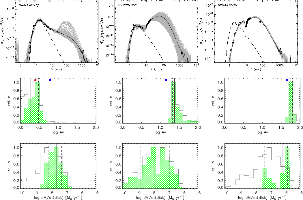 |
Figure A.3:
Examples of SED fits for three objects in our sample with
[Ne II] detections. From left to right: DoAr25/GY17, WL20/GY240, and
IRS44/GY269. The first is classified as Stage/Class II, the other two as
Stage/Class I. The upper row shows the SEDs and the best fit models as
produced by the Web interface provided by Robitaille et al. (2006). For the
datapoints, detections and upper limits are indicated by circles and
triangles, respectively. The lower two rows represent distributions of
two fit parameters, |
| Open with DEXTER | |
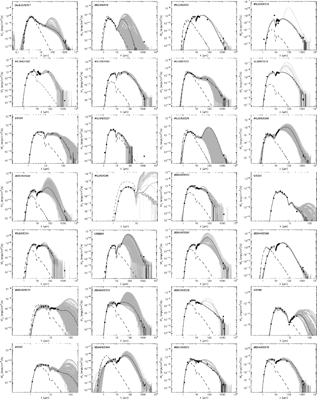 |
Figure A.4: SEDs and best fit models, as produced by the Web interface provided by Robitaille et al. (2006), for the 28 YSOs in our sample. |
| Open with DEXTER | |
Following visual examination of the SED fits and of the distributions
of model parameters used to define the confidence intervals, we
decided to modify the input datapoints for two objects: for
IRS45/GY273 we excluded the 1.2 and 1.3 mm datapoints from
Stanke et al. (2006) and Andre & Montmerle (1994); including these
points significantly worsened the quality of the fit and had a
significant effect on the values of the parameters. The 1.2 mm flux
is >20 times higher than the 1.3 mm flux (an upper limit) and
can probably be attributed to an extended source that includes
our YSO. For GY289, a source with average IRS flux <0.5 Jy, we
decided to include the IRS datapoints because: i) they agree quite
well with the MIPS fluxes at similar wavelengths; ii) the quality of
the model fit is reasonable (
![]() )
and; iii) the
confidence intervals of the model parameters are narrower but
compatible with those from the fit performed without these points.
)
and; iii) the
confidence intervals of the model parameters are narrower but
compatible with those from the fit performed without these points.
For one object, WL5/GY246, we could not obtain a unique fit with the above procedure. The object was previously classified as a deeply absorbed Class III star with an F7 spectral type (Greene & Meyer 1995), and our SED was defined by J, H, K, Spitzer IRAC 1-4 and 1.2/1.3 mm fluxes. Fits both with and without the mm fluxes, likely contaminated by nearby sources (cf. Stanke et al. 2006; Andre & Montmerle 1994), consistently yield high envelope and/or disk accretion rates, typical of a Class I object, but having little effect on the NIR/MIR part of the SED due to the associated large inner disk radii. The NIR/MIR SED can however be fit equally well by purely photospheric ``Phoenix'' models, as suggested by the same Robitaille et al. (2007) web interface used to fit the star/disk/envelope models. We thus decided to assume that WL5/GY246 is a Class III object and to derive its extinction, effective temperature, and stellar mass using the J, H, and K photometry, the spectral type, and the calibrations tabulated by Kenyon & Hartmann (1995). Uncertainties were estimated from the assumed uncertainty on the spectral type, one subclass, and the range of values obtained by estimating the absorption from the J-H, H-K, and J-K colors.
Table 3, introduced in the main text (Sect. 2.3), lists the outcome of the SED-fit process: the
quality of the fit (the ![]() of the ``best-fit'' model), the
object extinction (the sum of interstellar and envelope extinction),
the stellar effective temperature and mass, the disk mass, the disk
and envelope accretion rates, the evolutionary Stage. The last
quantity was assigned following Robitaille et al. (2007). Stage I:
of the ``best-fit'' model), the
object extinction (the sum of interstellar and envelope extinction),
the stellar effective temperature and mass, the disk mass, the disk
and envelope accretion rates, the evolutionary Stage. The last
quantity was assigned following Robitaille et al. (2007). Stage I:
![]() ;
Stage II:
;
Stage II:
![]() and
and
![]() ;
Stage III:
;
Stage III:
![]() and
and
![]() .
As indicated in the main
text, in order to use a designation more familiar to researchers in
the field, we also refer to the ``Stages'' as ``Classes''.
.
As indicated in the main
text, in order to use a designation more familiar to researchers in
the field, we also refer to the ``Stages'' as ``Classes''.
Figures A.5 and A.6 compare the
extinction values (![]() )
and stellar
)
and stellar
![]() obtained
from the SED fits with the same parameters listed in
Table 2 for Class II and Class III stars.
Given the considerable uncertainties of both determinations, the SED
fits yield results similar to those obtained with the method of
Natta et al. (2006). A similar comparison with the accretion rates derived
from the Pa
obtained
from the SED fits with the same parameters listed in
Table 2 for Class II and Class III stars.
Given the considerable uncertainties of both determinations, the SED
fits yield results similar to those obtained with the method of
Natta et al. (2006). A similar comparison with the accretion rates derived
from the Pa![]() and Br
and Br![]() NIR line fluxes (in
Table 2) is less conclusive due to the large number
of upper limits and to the large uncertainties that affect the
spectroscopic measurements as well as the SED fits. Seven objects can
be used for the comparison, having accretion rate estimates or upper
limits from both methods. For only two stars, both methods yield
estimates: those for IRS 54 are in good agreement; for WL 16 the
spectroscopic estimate is 2.6 dex higher than the value from the SED
fits,
NIR line fluxes (in
Table 2) is less conclusive due to the large number
of upper limits and to the large uncertainties that affect the
spectroscopic measurements as well as the SED fits. Seven objects can
be used for the comparison, having accretion rate estimates or upper
limits from both methods. For only two stars, both methods yield
estimates: those for IRS 54 are in good agreement; for WL 16 the
spectroscopic estimate is 2.6 dex higher than the value from the SED
fits,
![]()
![]() yr-1. The discrepancy is
however reduced to 1.2 dex when comparing the result of the SED fit
with the Natta et al. (2006) value. Moreover, the derivation of
yr-1. The discrepancy is
however reduced to 1.2 dex when comparing the result of the SED fit
with the Natta et al. (2006) value. Moreover, the derivation of ![]() from the Pa
from the Pa![]() line with the method of Natta et al. (2006, see also Sect. 2.3# is better suited for cool stars and is
likely to yield inaccurate results for WL 16 (
line with the method of Natta et al. (2006, see also Sect. 2.3# is better suited for cool stars and is
likely to yield inaccurate results for WL 16 (
![]() K). An independent estimate by Najita et al. (1996) yielded
an upper limit compatible with the SED value:
K). An independent estimate by Najita et al. (1996) yielded
an upper limit compatible with the SED value:
![]()
![]() yr-1. Three other stars have
yr-1. Three other stars have
![]() estimates from the SED fits and upper limits from
Table 2: in two cases, IRS 51 and IRS 47,
the confidence intervals from the SED fits are consistent with the
upper limits; for DoAr 25/GY17, the only star with optical
magnitudes, the SED fit yields an accretion rate that is 1.6 dex
higher than the upper limit from the Pa
estimates from the SED fits and upper limits from
Table 2: in two cases, IRS 51 and IRS 47,
the confidence intervals from the SED fits are consistent with the
upper limits; for DoAr 25/GY17, the only star with optical
magnitudes, the SED fit yields an accretion rate that is 1.6 dex
higher than the upper limit from the Pa![]() line. Finally, for two
stars, WL 10 and WL 11, the spectroscopic estimates are 0.4 dex and
0.1 dex larger than the upper limits from the SED fits. The
discrepancy is however reduced to 0.24 dex for WL 10 and disappears
for WL 11 if the slightly larger
line. Finally, for two
stars, WL 10 and WL 11, the spectroscopic estimates are 0.4 dex and
0.1 dex larger than the upper limits from the SED fits. The
discrepancy is however reduced to 0.24 dex for WL 10 and disappears
for WL 11 if the slightly larger ![]() values from Natta et al. (2006)
are considered instead of those in Table 2.
values from Natta et al. (2006)
are considered instead of those in Table 2.
A.3 Summary
In this Appendix we have shown that the SED models of Robitaille et al. (2006), although undeniably approximate, can be useful to constrain parameters such as the line-of-sight absorption and the disk accretion rate, even in the absence of optical photometry. Although resulting uncertainties in these parameters are often large, the constraints are by and large compatible with independent determinations obtained with more direct methods.
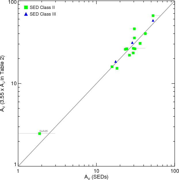 |
Figure A.5:
Comparison of the |
| Open with DEXTER | |
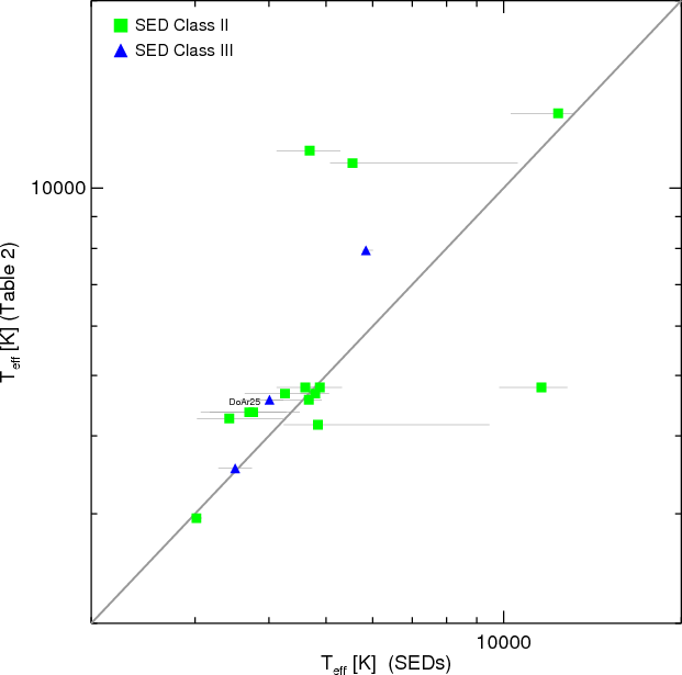 |
Figure A.6: Same as Fig. A.5 for the effective temperatures. |
| Open with DEXTER | |
Table A.1: Flux densities, in mJy, collected from the literature (cf. Sect. A.2) and used for the SED fits.
Table A.2: Flux densities, in Jy, obtained from the IRS spectra for the SED fits.
Current usage metrics show cumulative count of Article Views (full-text article views including HTML views, PDF and ePub downloads, according to the available data) and Abstracts Views on Vision4Press platform.
Data correspond to usage on the plateform after 2015. The current usage metrics is available 48-96 hours after online publication and is updated daily on week days.
Initial download of the metrics may take a while.