| Issue |
A&A
Volume 504, Number 3, September IV 2009
|
|
|---|---|---|
| Page(s) | 821 - 828 | |
| Section | Extragalactic astronomy | |
| DOI | https://doi.org/10.1051/0004-6361/200912237 | |
| Published online | 16 July 2009 | |
Online Material
Appendix A: Log-parabolic spectra
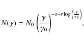
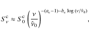
In this Appendix we show how electron populations with a log-parabolic energy distribution of the form expressed by Eq. (3), that is,
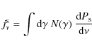
emit log-parabolic spectra via the SSC process. The related particle synchrotron emissivity
 |
(A.2) |
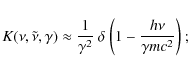
is easily computed on using the close approximation to the single particle emission in the shape of a delta-function (see Rybicki & Lightmann 1979), that is,
 |
(A.3) |
and to a SED again of log-parabolic shape
 |
(A.4) |
its slope at the synchrotron reference frequency
 |
(A.5) |
the spectral curvature by
and the peak value
For IC radiation in the Thomson regime we may write to a fair approximation
![]() (see Rybicky & Lightmann 1979) where
(see Rybicky & Lightmann 1979) where
![]() is the power radiated by a single-particle IC scattering in the Thomson regime, having denoted with
is the power radiated by a single-particle IC scattering in the Thomson regime, having denoted with
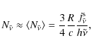
![]() the synchrotron radiation density
the synchrotron radiation density![]() . We obtain once again a log-parabolic SED
. We obtain once again a log-parabolic SED
 |
(A.7) |
where the slope at the IC reference frequency
 |
(A.8) |
and the spectral curvature reads
The peak value
For the Klein-Nishina (KN) regime instead it necessary to consider the convolution
 |
(A.10) |
where
 |
(A.11) |
on approximating
 |
(A.12) |
one obtains again a SED with a log-parabolic shape
 |
(A.13) |
Now the slope at
| (A.14) |
is steeper, and the spectral curvature
is larger than in the Thomson regime. The peak value
The transition between the two regimes occurs when
![]() ,
where
,
where
![]() ,
that is, when
,
that is, when
 |
(A.16) |
holds, or equivalently
 |
(A.17) |
We close these calculations with two remarks. First, the (primed) quantities used here refer to the rest frame of the emitting region, while the observed (unprimed) quantities must be multiplied by powers of the beaming factor
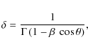 |
(A.18) |
Appendix B: Particle acceleration processes
![\begin{figure}
\par\includegraphics[width=9cm,clip]{12237fg7.eps}
\end{figure}](/articles/aa/olm/2009/36/aa12237-09/img232.png) |
Figure B.1:
Example of time evolution of the
|
| Open with DEXTER | |
![\begin{figure}
\par\includegraphics[width=9cm,clip]{12237fg8.eps}
\end{figure}](/articles/aa/olm/2009/36/aa12237-09/img233.png) |
Figure B.2:
Example of time evolution of the
|
| Open with DEXTER | |
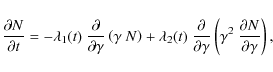
Here we derive a log-parabolic electron energy distribution
![]() from a kinetic continuity equation of the Fokker-Planck type; following Kardashev (1962), in the jet rest frame this reads
from a kinetic continuity equation of the Fokker-Planck type; following Kardashev (1962), in the jet rest frame this reads
where
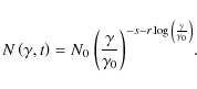
The Fokker-Planck Eq. (B.1) describes the evolution of the electron distribution function; with an initially mono-energetic distribution in the form of a delta-function
![]() (n is the initial particle number density) the solution at subsequent times t takes the form of the log-parabolic energy distribution assumed in Eq. (3) of the main text (see also A.1), reading
(n is the initial particle number density) the solution at subsequent times t takes the form of the log-parabolic energy distribution assumed in Eq. (3) of the main text (see also A.1), reading
Here the time depending slope at
 |
(B.3) |
meanwhile, the curvature of
 |
(B.4) |
from the large initial values corresponding to the initially mono-energetic distribution. Correspondingly, the time-dependent height at
![\begin{displaymath}N_0=\frac{1}{2\sqrt{\pi}}\frac{n}{\gamma_0}\frac{1} {\sqrt{\i...
...mbda_2}}\right)}^2}
{4\int{{\rm d}t~\lambda_2}}}\right]}}\cdot
\end{displaymath}](/articles/aa/olm/2009/36/aa12237-09/img250.png) |
(B.5) |
To wit, Eq. (B.2) describes the evolution of the electron distribution, growing broader and broader under the effect of stochastic acceleration, while its peak moves from
 |
(B.6) |
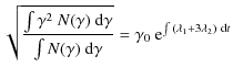
under the contrasting actions of the systematic and stochastic accelerations. An important quantity to focus on for the emission properties is the rms energy
| |
 |
||
| = | (B.7) |
which is also the position for the peak of the distribution
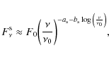
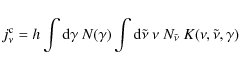
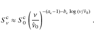
We have already derived in Appendix A the shapes of the spectra (synchrotron, and IC in both the Thomson and KN regimes) emitted by the distribution given in Eq. (3); here we stress the time dependence of their main spectral features. We can write for the synchrotron emission![]()
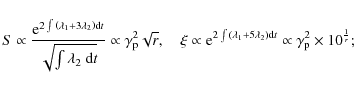
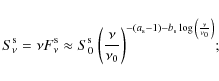
for IC emission we have in the Thomson regime
 |
(B.9) |
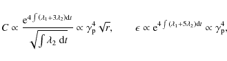
and in the extreme KN regime
Note that during flares, since
Now we focus the above relations for the simple case of time independent ![]() and
and ![]() ,
when
,
when
![]() ;
then we have
;
then we have
while for the rms energy we have
so for the peak frequency and the spectral curvature we have
where
The value of ![]() can be evaluated from observing the synchrotron spectral curvatures b2 and b1 at two times t2 and t1, respectively (recall that
can be evaluated from observing the synchrotron spectral curvatures b2 and b1 at two times t2 and t1, respectively (recall that
![]() ); denoting with t2 - t1 this time interval, we have
); denoting with t2 - t1 this time interval, we have
 |
(B.14) |
on the other hand, form observing the related synchrotron peaks
![\begin{displaymath}\lambda_1=\left[{\frac{1}{2\left({t_2 - t_1}\right)}\ln{\left...
...{1}{r_2}-\frac{1}{r_1}}\right)}\right] \frac{1+z}{\delta}\cdot
\end{displaymath}](/articles/aa/olm/2009/36/aa12237-09/img271.png) |
(B.15) |
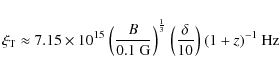
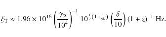
For example, in the case of Mrk 501 in the states of 7 and 16 April 1997, we obtain (on assuming
If the total energy available to the jet is limited (e.g., by the BZ limit, see text) we expect that
![]() and
and
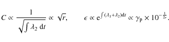
![]() cannot grow indefinitely, but are to attain a limiting value. At low energies where
cannot grow indefinitely, but are to attain a limiting value. At low energies where
![]() holds, we have
holds, we have
![]() and
and
![]() as before; at higher energies when
as before; at higher energies when
![]() reaches its limit,
reaches its limit,
![]() holds, leading to
holds, leading to
![]() and
and
![]() .
Eventually also
.
Eventually also
![]() reaches its limit, and both the fluxes and the peak frequencies cannot grow any more.
reaches its limit, and both the fluxes and the peak frequencies cannot grow any more.
Appendix C: Prefactors for Eqs. (4)-(13)
The HSZ SSC model is, as stated before, characterized by five parameters: the rms particle energy
![]() ,
the particle density n, the magnetic field B, the size of the emitting region R and the beaming factor
,
the particle density n, the magnetic field B, the size of the emitting region R and the beaming factor ![]() .
So the model may be constrained by five observables that we denote with
.
So the model may be constrained by five observables that we denote with
 |
(C.1) |
 |
(C.2) |
where the indexes i,j,k,h express the normalizations demonstrated below; in addition, we denote with
In the Thomson regime we find
| B | = | ||
| (C.3) | |||
| = | 13.5 | ||
| (C.4) | |||
| R | = | ||
| (C.5) | |||
| n | = | ||
| (C.6) | |||
| = | (C.7) |
For the extreme KN regime we obtain
| B | = | ||
| (C.8) | |||
| = | |||
| (C.9) | |||
| R | = | ||
| (C.10) | |||
| n | = | ||
| (C.11) | |||
| = | |||
| (C.12) |
Current usage metrics show cumulative count of Article Views (full-text article views including HTML views, PDF and ePub downloads, according to the available data) and Abstracts Views on Vision4Press platform.
Data correspond to usage on the plateform after 2015. The current usage metrics is available 48-96 hours after online publication and is updated daily on week days.
Initial download of the metrics may take a while.