| Issue |
A&A
Volume 504, Number 3, September IV 2009
|
|
|---|---|---|
| Page(s) | 821 - 828 | |
| Section | Extragalactic astronomy | |
| DOI | https://doi.org/10.1051/0004-6361/200912237 | |
| Published online | 16 July 2009 | |
SSC radiation in BL Lacertae sources, the end of the tether![[*]](/icons/foot_motif.png)
A. Paggi1 - F. Massaro2 - V. Vittorini3 - A. Cavaliere1 - F. D'Ammando1,3 - F. Vagnetti1 - M. Tavani1,3
1 - Dipartimento di Fisica, Università di Roma Tor Vergata, Via della Ricerca Scientifica 1, 00133 Roma, Italy
2 -
Harvard, Smithsonian Astrophysical Observatory, 60 Garden Street, Cambridge, MA 02138, USA
3 -
INAF, via Fosso del Cavaliere 1, 00100 Roma, Italy
Received 31 March 2009 / Accepted 12 July 2009
Abstract
Context. The synchrotron-self Compton (SSC) radiation process is widely held to provide a close representation of the double peaked spectral energy distributions from BL Lac Objects (BL Lacs). This subclass of Active Galactic Nuclei is marked by non-thermal beamed radiations, highly variable on timescales of days or less. Their outbursts in the ![]() rays relative to the optical/X rays might be surmised to be enhanced in BL Lacs as these photons are upscattered via the inverse Compton (IC) process.
rays relative to the optical/X rays might be surmised to be enhanced in BL Lacs as these photons are upscattered via the inverse Compton (IC) process.
Aims. From the observed correlations among the spectral parameters (peak frequencies, fluxes and curvature) during optical/X-ray variations we aim at predicting corresponding correlations in the ![]() -ray band, and the actual relations between the
-ray band, and the actual relations between the ![]() -ray and the X-ray variability consistent with the SSC emission process.
-ray and the X-ray variability consistent with the SSC emission process.
Methods. We start from the homogeneous single-zone SSC source model, with log-parabolic energies distributions of emitting electron as required by the X-ray data of many sources. We find relations among spectral parameters of the IC radiation in both the Thomson (for Low energy BL Lacs) and the Klein-Nishina regimes (mainly for High energy BL Lacs); whence we compute how variability is driven by a smooth increase of key source parameters, primarily the root mean square electron energy.
Results. In the Klein-Nishina regime the model predicts for HBLs lower inverse Compton fluxes relative to synchrotron, and milder ![]() -ray relative to X-ray variations. Stronger
-ray relative to X-ray variations. Stronger ![]() -ray flares observed in some HBLs like Mrk 501 are understood in terms of additional, smooth increases also of the emitting electron density. However, episodes of rapid flares as recently reported at TeV energies are beyond the reach of the single component SSC model with one dominant varying parameter. Furthermore, spectral correlations at variance with our predictions, as well as TeV emissions in LBL objects (like BL Lacertae itself) cannot be explained in terms of the simple HSZ SSC model, and in these cases the source may require additional electron populations in more elaborate structures like decelerated relativistic outflows or sub-jet scenarios.
-ray flares observed in some HBLs like Mrk 501 are understood in terms of additional, smooth increases also of the emitting electron density. However, episodes of rapid flares as recently reported at TeV energies are beyond the reach of the single component SSC model with one dominant varying parameter. Furthermore, spectral correlations at variance with our predictions, as well as TeV emissions in LBL objects (like BL Lacertae itself) cannot be explained in terms of the simple HSZ SSC model, and in these cases the source may require additional electron populations in more elaborate structures like decelerated relativistic outflows or sub-jet scenarios.
Conclusions. We provide a comprehensive benchmark to straightforwardly gauge the capabilities and effectiveness of the SSC radiation process. The single component SSC source model in the Thomson regime turns out to be adequate for many LBL sources. In the mild Klein-Nishina regime it covers HBL sources undergoing variations driven by smooth increase of a number of source parameters. However, the simple model meets its limits with the fast/strong flares recently reported for a few sources in the TeV range; these clearly require sudden accelerations of emitting electrons in a second source component.
Key words: galaxies: active - galaxies: jets - BL Lacertae objects: general - radiation mechanisms: non-thermal
1 Introduction
Blazars are among the brightest Active Galactic Nuclei (AGNs) observed, with inferred (isotropic) luminosities up to
![]() .
Actually these sources are widely held to be AGNs radiating from a relativistic jet closely aligned to the observer line of sight; this emits non-thermal radiations with observed fluxes enhanced by relativistic effects so as to often overwhelm other, thermal or reprocessed emissions.
.
Actually these sources are widely held to be AGNs radiating from a relativistic jet closely aligned to the observer line of sight; this emits non-thermal radiations with observed fluxes enhanced by relativistic effects so as to often overwhelm other, thermal or reprocessed emissions.
BL Lacs in particular are Blazars showing no or just weak emission lines. Their spectra may be represented as a continuous spectral energy distribution (SED)
![]() marked by two peaks: a lower frequency one, widely interpreted as synchrotron emission by highly relativistic electrons; and a higher frequency counterpart, believed to be inverse Compton upscattering by the same electrons of seed photons either emitted by an external source (external Compton, EC, see e.g. Sikora et al. 1994), or provided by the photons of the very synchrotron radiation (synchrotron-self Compton, SSC; see, e.g., Marscher & Gear 1985; Maraschi et al. 1992).
marked by two peaks: a lower frequency one, widely interpreted as synchrotron emission by highly relativistic electrons; and a higher frequency counterpart, believed to be inverse Compton upscattering by the same electrons of seed photons either emitted by an external source (external Compton, EC, see e.g. Sikora et al. 1994), or provided by the photons of the very synchrotron radiation (synchrotron-self Compton, SSC; see, e.g., Marscher & Gear 1985; Maraschi et al. 1992).
The BL Lacs are usually classified in terms of the frequency of their synchrotron peak (see Padovani & Giommi 1995): for the low frequency BL Lacs (LBLs) the peak lies in the infrared-optical bands, while the inverse Compton (IC) component peaks at MeV energies; instead, high frequency BL Lacs (HBLs) feature a first peak in the X-ray band and the second one at
![]() energies or beyond; intermediate frequency BL Lacs (IBLs) stand in the middle, with the first peak at optical frequencies and the second peak at
energies or beyond; intermediate frequency BL Lacs (IBLs) stand in the middle, with the first peak at optical frequencies and the second peak at ![]() 1 GeV.
1 GeV.
BL Lac Objects also show rapid variability on timescales of days or shorter, during which the sources undergo strong flux variations often named ``flares''.
The homogeneous single zone (HSZ) SSC model (based, in particular, on a single electron population) constitutes an attractively simple source structure worth to be extensively tested and pushed to its very limits, as we discuss below; following Katarzynski et al. (2005), Tramacere et al. (2007), we focus on deriving the simultaneous changes of the synchrotron and IC fluxes of BL Lacs to be expected from an updated version of SSC. We use a realistic log-parabolic energy distribution of the electrons radiating the synchrotron photons and upscattering them by IC in either the Thomson or the Klein Nishina (KN) regime.
2 Background relations
2.1 Log-parabolic electron distribution and spectra
The SEDs of BL Lacs exhibit two distinct peaks or humps. To describe these in detail a number of spectral models have been used over the years: power-laws with an exponential cutoff, broken power-laws, or spectra curved in the shape of a log-parabola. The latter are being increasingly used, as they generally provide more accurate fits than broken power-laws in the optical X-ray bands, with residuals uniformly low throughout a wide energy range (see discussion by
Landau et al. 1986; Tanihata et al. 2004; Massaro et al. 2004a; Tramacere et al. 2007; Nieppola et al. 2006; Donnarumma et al. 2009)![]() .
.
So we adopt log-parabolae in view of their optimal performance as a precise fitting tool. Moreover, they are also effective in yielding simple, analytical expressions (given in their exact form in Appendix A, following Eqs. (A.6), (A.9) and (A.15)) for peak frequencies and fluxes in both in the inverse Compton regimes, Thomson and Klein-Nishina. Finally, the physically interesting feature of log-parabolic spectra is their direct link to the acceleration processes of the emitting particles; in fact, as shown in Appendix B, log-parabolic emitted spectra simply relate to log-parabolic particle energy distributions, that in turn naturally arise from systematic and stochastic acceleration processes as dealt with by the Fokker-Planck equation.
Thus for the synchrotron SED we write
here
An analogous expression holds for the inverse Compton radiation
which in the Thomson regime the IC has less curved spectra with
Such spectra are radiated by electron populations with a log-parabolic energy distribution, namely
The result is easily inferred and straightforward to compute on using the delta-function approximations for the single particle emissions (see Appendix A); it is found to hold also for the exact shape of the latter with the numerical simulations outlined in Fig. 1, and reported in full detail in Figs. B.1 and B.2.
![\begin{figure}
\par\includegraphics[width=9cm,clip]{12237fg1.eps}
\end{figure}](/articles/aa/full_html/2009/36/aa12237-09/img40.png) |
Figure 1:
Two examples of exact, steady SEDs provided by numerical simulations (code by Massaro 2007) after the HSZ SSC model from relativistic electrons with a log-parabolic energy distribution
|
| Open with DEXTER | |
Table 1: Source parameters for some BL Lac sources.
2.2 Source parameters
Using the previous scalings, with the relation
![]() between the observed variation time
between the observed variation time ![]() and the size R of the emitting region (assuming spherical symmetry in the rest frame), we obtain relations of source parameters with the observables. In the Thomson regime we find
and the size R of the emitting region (assuming spherical symmetry in the rest frame), we obtain relations of source parameters with the observables. In the Thomson regime we find
For the extreme KN regime we find instead:
Note that a delay of the order of
Numerical values for the prefactors are given in Appendix C, where normalizations are chosen referring to a typical LBL source with
![]() ,
,
![]() ,
,
![]() ,
,
![]() ;
and to a typical HBL source with
;
and to a typical HBL source with
![]() ,
,
![]() ,
,
![]() ,
,
![]() .
Values of physical parameters for some sources are given in Table 1. Note that the simple Eqs. (4)-(8) provide parameter values in close agreement with the ones needed to fit the observations of LBL or IBL sources in Thomson regime; on the other hand the extreme KN limit underlying Eqs. (9)-(13) would yield disagreement for HBLs, indicating that these sources just border the KN regime.
.
Values of physical parameters for some sources are given in Table 1. Note that the simple Eqs. (4)-(8) provide parameter values in close agreement with the ones needed to fit the observations of LBL or IBL sources in Thomson regime; on the other hand the extreme KN limit underlying Eqs. (9)-(13) would yield disagreement for HBLs, indicating that these sources just border the KN regime.
We evaluate the position
![]() of the synchrotron peak when the transition between the two IC regimes occurs, to find
of the synchrotron peak when the transition between the two IC regimes occurs, to find
or equivalently
So we conclude that in LBLs, which feature the synchrotron peak at optical/IR frequencies with
2.3 Spectral correlations during X-ray spectral variations
Correlations in the synchrotron emission between S and ![]() with
with ![]() can be used to pinpoint the main driver of the spectral changes during X-ray variations (see also Tramacere et al. 2007). In fact, the synchrotron SED peak scales (for nearly constant spectral curvature as anticipated in Sect. 2.1)
as
can be used to pinpoint the main driver of the spectral changes during X-ray variations (see also Tramacere et al. 2007). In fact, the synchrotron SED peak scales (for nearly constant spectral curvature as anticipated in Sect. 2.1)
as
![]() at the peak frequency itself scaling as
at the peak frequency itself scaling as
![]() .
.
Thus on writing the dependence of S on ![]() in the form of a powerlaw
in the form of a powerlaw
![]() ,
we expect
,
we expect
![]() to apply when the spectral changes are driven mainly by variations of the electrons rms energy;
to apply when the spectral changes are driven mainly by variations of the electrons rms energy;
![]() for dominant changes of the magnetic field;
for dominant changes of the magnetic field;
![]() if changes in the beaming factor dominate;
if changes in the beaming factor dominate;
![]() formally applies for changes only in the number density of the emitting particles. Results by the latter authors focus on
formally applies for changes only in the number density of the emitting particles. Results by the latter authors focus on
![]() and B as dominant drivers.
Starting from such correlations we aim at predicting the expected correlations and flux variations in the
and B as dominant drivers.
Starting from such correlations we aim at predicting the expected correlations and flux variations in the ![]() -ray band.
-ray band.
Particle rms energy variations are of particular interest because they naturally arise as a consequence of systematic plus stochastic acceleration of the electron population (details in Appendix B).
3  -ray spectra
3.1 Spectral correlations
The above results lead us to expect specific correlations between SED peak frequencies and fluxes as follows. In the case of dominant rms particle energy variations we expect for the synchrotron emission
while for the IC we have
| (17) |
for LBL objects, and
| (18) |
for extreme HBLs.
In the case of magnetic field variations we have for the synchrotron emission
| (19) |
while for the IC we have
| (20) |
for LBL objects, and
formally with
![\begin{figure}
\par\includegraphics[width=9cm,clip]{12237fg2.eps}
\end{figure}](/articles/aa/full_html/2009/36/aa12237-09/img98.png) |
Figure 2: To illustrate the differences of the IC SEDs in the Thomson and in the extreme KN regime, we show the results of numerical simulations (code by Massaro 2007) after the HSZ SSC model, for different sources with larger and larger rms energy of the radiating particles and other parameters kept constant (including the curvature of the particle energy distribution). The vertical line indicates the frequency of the synchrotron peak where the IC scattering changes over the Thomson to the KN regime (see Eq. (14)). Actual sources in their evolution (represented in Figs. B.1 and B.2) vary their spectral curvature somewhat and only span a limited range in frequency and flux to the left (LBLs) or to the right (HBLs) of the line, with only the IBLs likely to cross it. |
| Open with DEXTER | |
To complete the above picture, we consider how saturation affects correlations. Denoting the total number of particles with ![]() ,
in the jet frame we have for the synchrotron luminosity
,
in the jet frame we have for the synchrotron luminosity
![]() ,
while for IC luminosity we have
,
while for IC luminosity we have
![]() and
and
![]() in Thomson and KN regime, respectively. Consider the case where the total power available to the jet is limited, e.g., in the BZ mechanism (Blandford & Znajek 1977) of power extraction from a maximally rotating black hole with an extreme, radiation pressure dominated disk that holds the pressure of the magnetic field facing the black hole horizon (see discussion by Cavaliere & D'Elia 2002, and references therein). Then the power has an upper bound
in Thomson and KN regime, respectively. Consider the case where the total power available to the jet is limited, e.g., in the BZ mechanism (Blandford & Znajek 1977) of power extraction from a maximally rotating black hole with an extreme, radiation pressure dominated disk that holds the pressure of the magnetic field facing the black hole horizon (see discussion by Cavaliere & D'Elia 2002, and references therein). Then the power has an upper bound
![]() ;
as a consequence, we expect an effect of saturation on the SED peaks as the emitted power, which represents a substantial fraction of the total jet power (see Ghisellini et al. 2008), approaches
;
as a consequence, we expect an effect of saturation on the SED peaks as the emitted power, which represents a substantial fraction of the total jet power (see Ghisellini et al. 2008), approaches
![]() .
For the total power, including radiative, kinetic and magnetic components,
.
For the total power, including radiative, kinetic and magnetic components,
![]() we envisage
we envisage
![]() ,
that is, the particles effectively accelerated to the increasing
,
that is, the particles effectively accelerated to the increasing
![]() decrease in number on approaching the BZ limit.
decrease in number on approaching the BZ limit.
The data analyses by Tramacere et al. (2007, 2009) for the variations of Mrk 421 are consistent with the beginning of such a saturation effect, as they show a declining value of ![]() when the peak moves toward the highest energies and approaches
when the peak moves toward the highest energies and approaches
![]() .
Partial saturation effects can also be explained in terms of systematic and stochastic acceleration processes; in particular, when the stochastic prevails over the systematic acceleration (as is bound to occur at high energies, see Appendix A) we expect
.
Partial saturation effects can also be explained in terms of systematic and stochastic acceleration processes; in particular, when the stochastic prevails over the systematic acceleration (as is bound to occur at high energies, see Appendix A) we expect ![]() to decrease toward 0.6, i.e.
to decrease toward 0.6, i.e.
![]() .
.
3.2 Related variabilities
We now focus on related variabilities between IC and synchrotron fluxes; here we are mainly interested on increases of peak frequencies and fluxes, as driven by acceleration processes of the emitting particles or by a growing magnetic field (see also Katarzynski et al. 2005).
For LBLs, that radiate mostly in the Thomson regime, we predict from Eqs. (16)-(21) a quadratic or linear variation of C with respect to S, depending on the parameter that mainly drives source variations. That is to say, we expect
in the case of dominant particle rms energy variations, or
for dominant magnetic field variations (see also Figs. 2 and 4).
Instead, for HBLs that radiate closer to the Klein-Nishina regime, we obtain a weaker ![]() -ray variability due to the decreasing KN cross section, leading in the extreme to
-ray variability due to the decreasing KN cross section, leading in the extreme to
in case of dominant particle rms energy variations, or
for dominant magnetic field variations. Expected correlations are summarized in Table 2.
From Figs. 2 and 4 it is seen that the transition to the KN regime has three effects on the IC spectrum: first, it brakes the peak frequency increase, because the energy the photon can gain is limited to the total electron energy
![]() ;
second, it reduces the flux increase at the SED peak, as a consequence of reduced cross section; third, it increases the spectral curvature near the peak as a consequence of frequency compression.
;
second, it reduces the flux increase at the SED peak, as a consequence of reduced cross section; third, it increases the spectral curvature near the peak as a consequence of frequency compression.
Viceversa, variations observed in IC section of the spectrum are related via Eqs. (22)-(25) to variations expected in the synchrotron emission; in particular, in HBLs ![]() -ray variations ought to have enhanced counterparts in X rays.
-ray variations ought to have enhanced counterparts in X rays.
Up to now Figs. 2 and 4 may be interpreted as a collection of different sources or of unrelated states of a single source; henceforth we will focus on the interpretation in terms of evolution in a flaring source where the parameters vary in a continuous fashion; in particular,
![]() increases under the drive of systematic and stochastic electron accelerations, in keeping with the description in terms of a continuity or kinetic equation of the Fokker-Planck type as given in detail in Appendix B. Signatures of such an evolution are provided not only by continuous growth of the peak frequencies, but even more definitely by the irreversible decrease of the spectral curvature (in terms of time or frequency) under the drive of the stochastic acceleration, see Eq. (B.13) and the observations by Tramacere et al. (2007, 2009). In fact, for a single electron population the curvature is to slowly decrease or stay nearly constant on the timescale of the systematic acceleration. So a sudden increase of curvature signals the injection of a new population/component.
increases under the drive of systematic and stochastic electron accelerations, in keeping with the description in terms of a continuity or kinetic equation of the Fokker-Planck type as given in detail in Appendix B. Signatures of such an evolution are provided not only by continuous growth of the peak frequencies, but even more definitely by the irreversible decrease of the spectral curvature (in terms of time or frequency) under the drive of the stochastic acceleration, see Eq. (B.13) and the observations by Tramacere et al. (2007, 2009). In fact, for a single electron population the curvature is to slowly decrease or stay nearly constant on the timescale of the systematic acceleration. So a sudden increase of curvature signals the injection of a new population/component.
In the following we will neglect radiative cooling, which does not strongly affect the spectral shape around the peaks; such a process will be particularly relevant when the source, after flaring up, relaxes back to a lower state upon radiating away its excess energies from high frequencies downwards (see Appendix B).
Table 2:
Spectral correlations (for
![]() ). We have denoted with
). We have denoted with
![]() or (B) the variations driven by increases of rms electron energy or magnetic field, respectively.
or (B) the variations driven by increases of rms electron energy or magnetic field, respectively.
![\begin{figure}
\par\includegraphics[width=9cm,clip]{12237fg3.eps}
\end{figure}](/articles/aa/full_html/2009/36/aa12237-09/img127.png) |
Figure 3:
Computed changes of spectral parameters corresponding to extended increase of rms particle energy with the other source parameters kept constant. As functions of
|
| Open with DEXTER | |
![\begin{figure}
\par\includegraphics[width=9cm,clip]{12237fg4.eps}
\end{figure}](/articles/aa/full_html/2009/36/aa12237-09/img128.png) |
Figure 4: As in Fig. 2, we show SEDs obtained from numerical simulations (code by Massaro 2007) of HSZ SSC radiations, for different sources with larger and larger magnetic field B and other parameters kept constant. The vertical line again indicates the transition frequency from the Thomson to the KN regime (see Eq. (15)); as B increases, the IC scattering changes its regime, and reduced cross section yields similar compression effects as in Fig. 2. |
| Open with DEXTER | |
![\begin{figure}
\par\includegraphics[width=9cm,clip]{12237fg5.eps}
\end{figure}](/articles/aa/full_html/2009/36/aa12237-09/img130.png) |
Figure 5:
Computed changes of spectral parameters as driven by an extended increase of the magnetic field with the other source parameters kept constant. The black full line represents the value of the ratio
|
| Open with DEXTER | |
3.3 Specific sources
We have applied the above simple expectations to two sources, 0716+714 (IBL) and Mrk 501 (HBL), among the few to date to provide extended simultaneous coverage of two different source states in X rays and ![]() rays.
rays.
The first is widely considered to be an IBL. In the low state observed by Automatic Imaging Telescope (AIT) in November 14 1996, the synchrotron peak at about at about
![]() falls quite below the threshold frequency expressed by Eqs. (14) or (15), so we expect for this source the IC scattering to occur mostly in the Thomson regime; simultaneous
falls quite below the threshold frequency expressed by Eqs. (14) or (15), so we expect for this source the IC scattering to occur mostly in the Thomson regime; simultaneous ![]() -ray observations were carried out by EGRET. The high activity
state of the source is described by data relative to GASP project of the WEBT and AGILE-GRID observations of 2007 September 7-12 (see Fig. 6). The source has shown similarly low flux levels during EGRET observations (Tagliaferri et al. 2003); so for flares with short duty cycle, it is not unreasonable to evaluate variations between the two distant states in the absence of closer observations; curvature variation is not required to fit the data, as we expect at lower energies where systematic dominates the stochastic acceleration (see Appendix A).
As shown in Figs. 3 and 5, peak flux and frequency variations of 0716+714 appear to be in between the lines representing increasing rms particle energy and increasing magnetic field, and so they may be described in terms of HSZ SSC with simultaneous variations of these two parameters.
-ray observations were carried out by EGRET. The high activity
state of the source is described by data relative to GASP project of the WEBT and AGILE-GRID observations of 2007 September 7-12 (see Fig. 6). The source has shown similarly low flux levels during EGRET observations (Tagliaferri et al. 2003); so for flares with short duty cycle, it is not unreasonable to evaluate variations between the two distant states in the absence of closer observations; curvature variation is not required to fit the data, as we expect at lower energies where systematic dominates the stochastic acceleration (see Appendix A).
As shown in Figs. 3 and 5, peak flux and frequency variations of 0716+714 appear to be in between the lines representing increasing rms particle energy and increasing magnetic field, and so they may be described in terms of HSZ SSC with simultaneous variations of these two parameters.
For the HBL source Mrk 501 we consider the two states described by Massaro et al. (2006), with simultaneous BeppoSAX and CAT observations of April 7 and 16 1997.
To understand the behavior of this source, from Figs. 3 and 5 it is seen that variations of B alone are ineffective and require complementary n increase by a factor of about 30; variations of
![]() are adequate in the KN regime, and only require a complementary doubling of n (which by itself would yield
are adequate in the KN regime, and only require a complementary doubling of n (which by itself would yield
![]() in both scattering regimes) to yield higher
in both scattering regimes) to yield higher ![]() -ray flux increase. Note that in going to higher energies the spectral curvature decreases somewhat (from
-ray flux increase. Note that in going to higher energies the spectral curvature decreases somewhat (from
![]() to
to
![]() for the low and high state, respectively) in keeping with model predictions; such a behavior is interesting as it marks a smooth growth, if anything, in the number of emitting particles as contrasted with sudden, substantial re-injection of nearly monoenergetic electrons that would suddenly reverse the otherwise irreversible decrease of r and b. Such a smooth growth obtains in a scenario of an expanding blast-wave that progressively involves more electrons (see, e.g., Ostriker & McKee 1988; Lapi et al. 2005; Vietri 2006).
for the low and high state, respectively) in keeping with model predictions; such a behavior is interesting as it marks a smooth growth, if anything, in the number of emitting particles as contrasted with sudden, substantial re-injection of nearly monoenergetic electrons that would suddenly reverse the otherwise irreversible decrease of r and b. Such a smooth growth obtains in a scenario of an expanding blast-wave that progressively involves more electrons (see, e.g., Ostriker & McKee 1988; Lapi et al. 2005; Vietri 2006).
We stress that in HBL sources even small flux variations in ![]() rays are expected to have enhanced and observable counterparts in X rays. We suggest that such variations should be checked upon
rays are expected to have enhanced and observable counterparts in X rays. We suggest that such variations should be checked upon ![]() -ray ``alarms'', the inverse triggering relative to usual.
The absence of such lower energies counterparts will indicate, for example, a flare driven dominantly by a particle number density increase associated with a magnetic field decrease
-ray ``alarms'', the inverse triggering relative to usual.
The absence of such lower energies counterparts will indicate, for example, a flare driven dominantly by a particle number density increase associated with a magnetic field decrease
![]() ,
causing
,
causing
![]() but a decreasing synchrotron peak frequency; such a kind of flare may easily drown into the primary synchrotron component.
but a decreasing synchrotron peak frequency; such a kind of flare may easily drown into the primary synchrotron component.
![\begin{figure}
\par\includegraphics[width=9cm,clip]{12237fg6.eps}
\end{figure}](/articles/aa/full_html/2009/36/aa12237-09/img137.png) |
Figure 6: Spectral fit of two different states of the IBL source 0716+714. The low state (blue line) data are relative to 1996 November 14 simultaneous observation by AIT, BeppoSAX and EGRET; the high state (red line) data are relative to 2007 September 7-12 simultaneous observations by GASP-WEBT and AGILE-GRID (Tagliaferri et al. 2003; Chen et al. 2008). |
| Open with DEXTER | |
3.4 Limiting timescales
As shown in Appendix B, systematic and stochastic acceleration processes occur in the sources on timescales
![]() and
and
![]() ,
respectively.
Limits to the variability timescales
,
respectively.
Limits to the variability timescales ![]() relate to the apparent size of the emission region by
relate to the apparent size of the emission region by
![]() (see Sect. 2.2); rapid variations require small emitting sources, but these could be optically thick to the pair production process. In fact,
(see Sect. 2.2); rapid variations require small emitting sources, but these could be optically thick to the pair production process. In fact, ![]() -ray photons collide with less energetic ones to produce e
-ray photons collide with less energetic ones to produce e![]() pairs, and the cross section of this process tops at a value around
pairs, and the cross section of this process tops at a value around
![]() (where
(where
![]() is the Thomson cross section) when the
is the Thomson cross section) when the ![]() -ray photon frequency
-ray photon frequency ![]() and the target photons frequency
and the target photons frequency
![]() satisfy the relation
satisfy the relation
![]() .
.
For the ![]() rays to escape from the emitting region the source ``compactness'' intervenes and can set lower bounds on the beaming factor (Cavaliere & Morrison 1980; Massaro 2007; Begelman et al. 2008). In fact the optical depth for this process is expressed in terms of observational quantities (primed quantities refer to the jet rest frame) as
rays to escape from the emitting region the source ``compactness'' intervenes and can set lower bounds on the beaming factor (Cavaliere & Morrison 1980; Massaro 2007; Begelman et al. 2008). In fact the optical depth for this process is expressed in terms of observational quantities (primed quantities refer to the jet rest frame) as
 |
(26) |
where D is the source distance expressed in
![\begin{displaymath}\delta\geq {\left[{\frac{9}{20}\frac{\sigma_{\rm T}~h^{1+2\be...
...\beta}~\xi^\beta}{\Delta t}}\right]}^{\frac{1}{6+2\beta}}\cdot
\end{displaymath}](/articles/aa/full_html/2009/36/aa12237-09/img151.png) |
(27) |
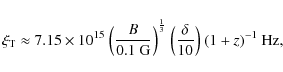
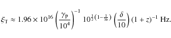
Thus rapid flux variations set a lower bound on the beaming factor; the highest bound between the previous relation and
The exponent ![]() contains a weak logarithmic dependence on
contains a weak logarithmic dependence on ![]() that may be neglected to a first approximation, and has a magnitude which depends on the source spectral properties; for definiteness, we use for b the typical value 0.2, and for
that may be neglected to a first approximation, and has a magnitude which depends on the source spectral properties; for definiteness, we use for b the typical value 0.2, and for
![]() .
For a LBL with
.
For a LBL with
![]() we obtain
we obtain
![]() ,
while for an extreme HBL with
,
while for an extreme HBL with
![]() ,
we obtain
,
we obtain
![]() .
A variation timescale
.
A variation timescale
![]() min for a LBL with
min for a LBL with
![]() implies
implies
![]() ,
while in an extreme HBL with
,
while in an extreme HBL with
![]() we find
we find
![]() .
.
In the specific case of PKS 2155-304 discussed by Begelman et al. (2008), the emitted power
![]() corresponds to
corresponds to
![]() ,
with
,
with
![]() ,
to give
,
to give
![]() and
and
![]() for
for
![]() min. We note that the source, even if widely considered a HBL, shows peculiar behaviors with respect to other TeV HBLs (see Massaro et al. 2008b); moreover, it does not satisfy the condition
min. We note that the source, even if widely considered a HBL, shows peculiar behaviors with respect to other TeV HBLs (see Massaro et al. 2008b); moreover, it does not satisfy the condition
![]() and so it cannot be considered an extreme HBL, as discussed below.
and so it cannot be considered an extreme HBL, as discussed below.
Extreme values of the beaming factor
![]() have been proposed to account for large peak separations
(Konopelko et al. 2003) or to explain very rapid spectral variations
(Begelman et al. 2008), formally with
have been proposed to account for large peak separations
(Konopelko et al. 2003) or to explain very rapid spectral variations
(Begelman et al. 2008), formally with
![]() min for the
min for the ![]() -ray flares of PKS 2155-304 in 2006 July 28 (Aharonian et al. 2007) and Mrk 501 in June 30 and July 9, 2007 (Albert et al. 2007a). Note that with BL Lac spectra realistically curved, the observed flux variations may be enhanced due to a slope effect best legible on the differential flux
-ray flares of PKS 2155-304 in 2006 July 28 (Aharonian et al. 2007) and Mrk 501 in June 30 and July 9, 2007 (Albert et al. 2007a). Note that with BL Lac spectra realistically curved, the observed flux variations may be enhanced due to a slope effect best legible on the differential flux ![]() ;
that is, when fluxes are measured at frequencies where the spectral slope is steep (as may be the case for PKS 2155-304), a strong observed flux variation implies only a mild variation of the peak flux and requires smaller values of
;
that is, when fluxes are measured at frequencies where the spectral slope is steep (as may be the case for PKS 2155-304), a strong observed flux variation implies only a mild variation of the peak flux and requires smaller values of ![]() .
Otherwise, a peak variation on a scale
.
Otherwise, a peak variation on a scale
![]() min would require in the SSC model
min would require in the SSC model
![]() for LBLs where
for LBLs where
![]() (see Eq. (7)), and
(see Eq. (7)), and
![]() for an extreme HBL where
for an extreme HBL where
![]() (see Eq. (12)).
(see Eq. (12)).
As stated under Sect. 3.3, in HBL sources even small flux variations in ![]() rays should have enhanced
counterparts in X rays. These may become hard to observe for example in a flare dominantly driven by particle number density increase associated with a magnetic field decrease (i.g., with
rays should have enhanced
counterparts in X rays. These may become hard to observe for example in a flare dominantly driven by particle number density increase associated with a magnetic field decrease (i.g., with
![]() ), leading to a synchrotron emission easily drowned into other components. On the other hand, components with
), leading to a synchrotron emission easily drowned into other components. On the other hand, components with
![]() appearing in an HBL spectrum go beyond the HSZ SSC model with variations of one dominant parameter, and therefore require a more elaborate source structure.
appearing in an HBL spectrum go beyond the HSZ SSC model with variations of one dominant parameter, and therefore require a more elaborate source structure.
In such cases the next natural scenarios are provided by decelerated relativistic outflows (Georganopoulos & Kazanas 2003), or by nested spine-layer jets (Tavecchio & Ghisellini 2008) and jets in a jet (Giannios et al. 2009).
4 Beyond the SSC
In Table 2 we have provided a comprehensive benchmark to gauge the performance of the HSZ SSC model for flaring BL Lac objects. This allows us to easily recognize events that may be accounted for within the model with physical variations of key source parameters, or that instead require more complex source structures.
Toward that purpose, we have used realistic log-parabolic spectral shapes produced by log-parabolic energy distributions of the emitting electrons, and studied IC radiation both in the Thomson and the Klein-Nishina regimes.
In the model we expect S to dominate C fluxes; in fact, moving to higher energies in a collection of different sources or in a prolonged evolution of a given source, we expect the emission to drift out of the pure Thomson and approach the KN regime, where the cross section decreases and limits the IC fluxes enforcing
![]() .
Such a relation is found to hold in a number of sources, and in particular in HBLs (see for example Tagliaferri et al. 2008).
.
Such a relation is found to hold in a number of sources, and in particular in HBLs (see for example Tagliaferri et al. 2008).
From Table 2 we stress here the source spectral variations predicted in ![]() rays. For LBLs, where the IC scattering mostly occurs in the Thomson regime, we recover the standard quadratic increase in
rays. For LBLs, where the IC scattering mostly occurs in the Thomson regime, we recover the standard quadratic increase in ![]() -ray fluxes with respect to IR-optical ones, expressed by
-ray fluxes with respect to IR-optical ones, expressed by
![]() for dominant particle rms energy variations (see Eq. (22)). Instead for HBLs, in which the IC scattering approaches the Klein-Nishina regime, we expect smaller or even vanishing increases of the
for dominant particle rms energy variations (see Eq. (22)). Instead for HBLs, in which the IC scattering approaches the Klein-Nishina regime, we expect smaller or even vanishing increases of the ![]() -ray flux relative to X rays, that is,
-ray flux relative to X rays, that is,
![]() for dominant particle rms energy variations (see Eq. (24)).
for dominant particle rms energy variations (see Eq. (24)).
Comparing with specific sources, we find the HSZ SSC model to be adequate for most LBLs at the present observational levels; whilst for example the HBL source Mrk 501 in April 1997 showed a ![]() -ray flux increase appreciably stronger than expected if it were dominated by just one driving parameter. We explain this behavior within the model in terms of an additional, smooth and moderate increase (by a factor around 2) in number density of the electrons responsible for the emission (see Sect. 3.3).
Such conditions can still be provided by a single electron population; this should be marked by a continuously decreasing spectral curvature b, as indicated by current data (Massaro et al. 2006), a feature providing a potentially powerful signature to closely check on further data. Instead, for dominant magnetic field variations we would expect
-ray flux increase appreciably stronger than expected if it were dominated by just one driving parameter. We explain this behavior within the model in terms of an additional, smooth and moderate increase (by a factor around 2) in number density of the electrons responsible for the emission (see Sect. 3.3).
Such conditions can still be provided by a single electron population; this should be marked by a continuously decreasing spectral curvature b, as indicated by current data (Massaro et al. 2006), a feature providing a potentially powerful signature to closely check on further data. Instead, for dominant magnetic field variations we would expect
![]() for LBL sources (see Eq. (23)), and
for LBL sources (see Eq. (23)), and
![]() for HBL sources (see Eq. 25)); but in that case the required increase in particle number density should be much higher by a factor of about 30, hard to interpret in terms of a single electron population.
for HBL sources (see Eq. 25)); but in that case the required increase in particle number density should be much higher by a factor of about 30, hard to interpret in terms of a single electron population.
On the other hand, on using the previous relations inversely, we see that even small ![]() -ray variations in HBL sources ought to have enhanced counterparts in the X rays, unless flare activity were driven by an additional jet component, for example one with higher magnetic field but lower particle density; thus the corresponding emission is easily overwhelmed by, or drowned into the main synchrotron, but then the rest frame acceleration times must be short enough to involve a significant fraction of the emitting region. We suggest this as a critical test for the simple model.
-ray variations in HBL sources ought to have enhanced counterparts in the X rays, unless flare activity were driven by an additional jet component, for example one with higher magnetic field but lower particle density; thus the corresponding emission is easily overwhelmed by, or drowned into the main synchrotron, but then the rest frame acceleration times must be short enough to involve a significant fraction of the emitting region. We suggest this as a critical test for the simple model.
Another limitation arises from rapid peak flux variations requiring large values of ![]() as shown in Sect. 3.4. In the extreme, the few sources with particularly fast
as shown in Sect. 3.4. In the extreme, the few sources with particularly fast ![]() -ray increases observed so far, like PKS 2155-304 in 2006 July 28 and Mrk 501 in June 30 and July 9, 2007 (see Sect. 3.4), require additional components with very high beaming factors that go definitely beyond the simple SSC model.
-ray increases observed so far, like PKS 2155-304 in 2006 July 28 and Mrk 501 in June 30 and July 9, 2007 (see Sect. 3.4), require additional components with very high beaming factors that go definitely beyond the simple SSC model.
Finally, another problem for the model arises from LBL objects showing substantial emissions in the GeV-TeV range that cannot be explained it terms of the simple HSZ SSC model (considering that second order IC scattering is negligible, see Massaro 2007) because the IC peak falls for these sources around
![]() ;
this may be the case for BL Lacertae itself (Albert et al. 2007b) and possibly similar sources like M87 (Georganopoulos et al. 2005) and Cen A (Lenian et al. 2008; Aharonian et al. 2009).
;
this may be the case for BL Lacertae itself (Albert et al. 2007b) and possibly similar sources like M87 (Georganopoulos et al. 2005) and Cen A (Lenian et al. 2008; Aharonian et al. 2009).
In all these cases the source may require more elaborate structure, like decelerated relativistic outflows or sub-jet scenarios (see Georganopoulos & Kazanas 2003; Tavecchio & Ghisellini 2008; Giannios et al. 2009). We stress that the injection of a second, monoenergetic electron population is expected to be marked by a sudden increase of the spectral curvature.
5 Discussion and conclusions
We propose that the sources of BL Lac type may be conveniently ordered in a succession spanning from smooth variations of one or a few dominant SSC parameter, up to the appearance of truly different components that ultimately break through the limits of the simple HSZ SSC model.
Even more so at increasing energies and frequencies,
that would imply weaker and weaker ![]() -ray fluxes relative to X-ray,
owing to KN cross section effects.
This picture is supported by the following two lines of evidence.
-ray fluxes relative to X-ray,
owing to KN cross section effects.
This picture is supported by the following two lines of evidence.
First, a recent statistical study of Third EGRET Catalogue data (Mukherjee et al. 2001; Casula 2008; Vagnetti et al., in prep.) shows for BL Lac objects observed at
![]() a weak
a weak ![]() -ray variability on average, compared to the FSRQ Blazars.
Also the time-structure functions for these two classes of objects indicate a similar trend, within the limitations of the sample.
-ray variability on average, compared to the FSRQ Blazars.
Also the time-structure functions for these two classes of objects indicate a similar trend, within the limitations of the sample.
Second, the first AGILE-GRID Catalogue of high confidence gamma-ray sources (Pittori et al. 2009) apparently shows few if any new BL Lac sources other than those already detected by EGRET. This circumstance suggests the sources observed by AGILE to be more powerful than the average; it leads to expect for the majority of the sources either reduced flare activity in this band, or weak average fluxes. We relate these features to reduced Klein-Nishina cross section that tends to limit both the average fluxes and the flares.
With Fermi, the first three months of observations Abdo et al. (2009) have yielded a substantial number of new BL Lac sources, and in particular a larger fraction of HBLs close to the ratio known from radio surveys (Nieppola et al. 2006). This is consistent with our expectations, considering the better instrumental sensitivity, especially at high energies generally favorable to the HBLs; for these sources we suggest to test the model's outcomes: C lower than S, and generally small (though possibly fast) flux variations compared to the LBLs
We plan to check our theoretical predictions against the public availability of the first year data from Fermi observations, and with simultaneous, multi-wavelength observations comparing the two basic subclasses of LBL and HBL of the BL Lac sources.
Acknowledgements
We thank our referee for useful comments and helpful suggestions. F. Massaro acknowledges the Foundation BLANCEFLOR Boncompagni-Ludovisi, née Bildt, for the grant awarded him in 2009 to support his research.
References
- Abdo, A. A., Ackermann, M., Ajello, M., et al. 2009, [arXiv:0902.1559] (In the text)
- Aharonian, F., Akhperjanian, A. G., Bazer-Bachi, A. R., et al. 2007, ApJ, 664, L71 [NASA ADS] [CrossRef] (In the text)
- Aharonian, F., Akhperjanian, A. G., Bazer-Bachi, A. R., et al. 2009,[arXiv:0903.1582] (In the text)
- Albert, J., Aliu, E., Anderhub, H., et al. 2007a, ApJ, 669, 862 [NASA ADS] [CrossRef] (In the text)
- Albert, J., Aliu, E., Anderhub, H., et al. 2007b. ApJ, 666, L17 (In the text)
- Begelman, M. C., Fabian, A., & Rees, M. J. 2008, MNRAS, 384, L19 [NASA ADS] (In the text)
- Blandford, R. D., & Znajek, R. L. 1977, MNRAS, 179, 433 [NASA ADS] (In the text)
- Bloom, S. D., & Marscher, A. P. 1996, ApJ, 461, 657 [NASA ADS] [CrossRef]
- Blumenthal, G. R., & Gould, R. J. 1970, Rev. Mod. Phys., 42, 237 [NASA ADS] [CrossRef]
- Casula, V. 2008, Thesis (In the text)
- Cavaliere, A., & D'Elia, V. 2002, ApJ, 571, 226 [NASA ADS] [CrossRef] (In the text)
- Cavaliere, A., & Morrison, P. 1980, ApJ, 238, L63 [NASA ADS] [CrossRef] (In the text)
- Chen, A. W., D'Ammando, F., Villata, M., et al. 2008, A&A, 489, L37 [NASA ADS] [CrossRef] [EDP Sciences] (In the text)
- Djannati-Atai, A., Piron, F., Barrau, A., et al. 1999, A&A, 350, 17 [NASA ADS] (In the text)
- Donnarumma, I., Vittorini, V., Vercellone. S., et al. 2009, ApJ, 691, L13 [NASA ADS] [CrossRef] (In the text)
- Fossati, G., Buckley, J. H., Bond, I. H., et al. 2008, ApJ, 677, 906 [NASA ADS] [CrossRef]
- Georganopoulos, M., & Kazanas, D. 2003, ApJ, 594, 27 [NASA ADS] [CrossRef] (In the text)
- Georganopoulos, M., Perlman, E. S., & Kazanas, D. 2005, ApJ, 634, L33 [NASA ADS] [CrossRef] (In the text)
- Giannios, D., Uzdensky, D. A., & Begelman, M. C. 2009, [arXiv:0901.1877]
- Giommi, P., Colafrancesco, S., Cutini, S., et al 2008, A&A, 487, L49 [NASA ADS] [CrossRef] [EDP Sciences]
- Inoue, S., & Takahara, F. 1996, ApJ, 463, 555 [NASA ADS] [CrossRef]
- Jones, F. C. 1968, Phys. Rev., 167, 1159 [NASA ADS] [CrossRef] (In the text)
- Kaplan, S. A. 1956, Sov. Phys., 2, 2 (In the text)
- Kardashev, N. S. 1962, SvA, 6, 317 [NASA ADS]
- Kataoka, J., Mattox, J. R., Quinn, J., et al. 1999, ApJ, 514, 138 [NASA ADS] [CrossRef]
- Katarzynski, K., Ghisellini, G., Tavecchio, F., et al. 2005, A&A, 433, 479 [NASA ADS] [CrossRef] [EDP Sciences]
- Konopelko, A., Mastichiadis, A., Kirk, J., et al. 2003, ApJ, 597, 851 [NASA ADS] [CrossRef] (In the text)
- Landau, R., Golisch, B., Jones, T., et al. 1986, ApJ, 308, 78 [NASA ADS] [CrossRef] (In the text)
- Lapi, A., Cavaliere, A., & Menci, N. 2005, ApJ, 619, 90 [NASA ADS] [CrossRef] (In the text)
- Lenain, J.-P., Boisson, C., & Sol, H. 2008, [arXiv:0807.2733] (In the text)
- Maraschi, L., Ghisellini, G., & Celotti, A. 1992, ApJ, 397, L5 [NASA ADS] [CrossRef] (In the text)
- Marscher, A. P. 1996, Energy Transport in Radio Galaxies and Quasars, ASP Conf. Ser., 100, 45
- Marscher, A. P., & Gear, W. K. 1985, ApJ, 298, 114 [NASA ADS] [CrossRef] (In the text)
- Massaro, F. 2007, Ph.D. Thesis (In the text)
- Massaro, E., Perri, M., Giommi, P., & Nesci, R. 2004a, A&A, 413, 489 [NASA ADS] [CrossRef] [EDP Sciences] (In the text)
- Massaro, E., Perri, M., Giommi, P., Nesci, R., & Verrecchia, F. 2004b, A&A, 422, 103 [NASA ADS] [CrossRef] [EDP Sciences] (In the text)
- Massaro, E., Tramacere, A., Perri, M., Giommi, P., & Tosti, G. 2006, A&A, 448, 861 [NASA ADS] [CrossRef] [EDP Sciences] (In the text)
- Massaro, F., Tramacere, A., Cavaliere, A., Perri, M., & Giommi, P. 2008a, A&A, 478, 395 [NASA ADS] [CrossRef] [EDP Sciences]
- Massaro, F., Giommi, P., Tosti, G., et al. 2008b, A&A, 489, 1047 [NASA ADS] [CrossRef] [EDP Sciences]
- Mukherjee, R., et al. 2001, in High Energy Gamma-Ray Astronomy, ed. F. A. Aharonian, & H. J. Völk (New York: AIP), AIP Conf. Proc., 558, 324 (In the text)
- Nieppola, E., Tornikoski, M., & Valtaoja, E. 2006, A&A, 445, 441 [NASA ADS] [CrossRef] [EDP Sciences] (In the text)
- Ostriker, J. P., & McKee, C. F. 1988, Rev. Mod. Phys., 61, 1 [NASA ADS] [CrossRef] (In the text)
- Padovani, P., & Giommi, P. 1995, ApJ, 444, 567 [NASA ADS] [CrossRef] (In the text)
- Paggi, A. 2007, Thesis (In the text)
- Pittori, C., Verrecchia, F., Chen, A. W., et al. 2009, [arXiv:0902.2959] (In the text)
- Rybicki, G. B., & Lightman, A. P. 1979, Radiative Processes in Astrophysics (New York: Wiley)
- Sikora, M., Begelman, M. C., & Rees, M. J. 1994, ApJ, 421, 123 [NASA ADS] [CrossRef] (In the text)
- Tagliaferri, G., Ravasio, M., & Ghisellini, G. 2003, A&A, 400, 477 [NASA ADS] [CrossRef] [EDP Sciences] (In the text)
- Tagliaferri, G., Foschini, L., Ghisellini, G., et al. 2008, ApJ, 679, 1029 [NASA ADS] [CrossRef] (In the text)
- Tanihata, C., Kataoka, J., Takahashi, T., et al. 2004, ApJ, 601, 759 [NASA ADS] [CrossRef] (In the text)
- Tavecchio, F., & Ghisellini, G. 2008, [arXiv:0810.0134] (In the text)
- Tavecchio, F., Maraschi, L., & Ghisellini, G. 1998, ApJ, 509, 608 [NASA ADS] [CrossRef]
- Tramacere, A., Massaro, F., & Cavaliere, A. 2007, A&A, 466, 521 [NASA ADS] [CrossRef] [EDP Sciences] (In the text)
- Tramacere, A., Giommi, P., Perri, M., Verrecchia, F., & Tosti, G. 2009, [arXiv:0901.4124v1]
- Vietri, M. 2006, Astrofisica delle alte energie, Torino, Bollati Boringhieri (In the text)
Online Material
Appendix A: Log-parabolic spectra
In this Appendix we show how electron populations with a log-parabolic energy distribution of the form expressed by Eq. (3), that is,
emit log-parabolic spectra via the SSC process. The related particle synchrotron emissivity
 |
(A.2) |
is easily computed on using the close approximation to the single particle emission in the shape of a delta-function (see Rybicki & Lightmann 1979), that is,
 |
(A.3) |
and to a SED again of log-parabolic shape
 |
(A.4) |
its slope at the synchrotron reference frequency
 |
(A.5) |
the spectral curvature by
and the peak value
For IC radiation in the Thomson regime we may write to a fair approximation
![]() (see Rybicky & Lightmann 1979) where
(see Rybicky & Lightmann 1979) where
![]() is the power radiated by a single-particle IC scattering in the Thomson regime, having denoted with
is the power radiated by a single-particle IC scattering in the Thomson regime, having denoted with
![]() the synchrotron radiation density
the synchrotron radiation density![]() . We obtain once again a log-parabolic SED
. We obtain once again a log-parabolic SED
 |
(A.7) |
where the slope at the IC reference frequency
 |
(A.8) |
and the spectral curvature reads
The peak value
For the Klein-Nishina (KN) regime instead it necessary to consider the convolution
 |
(A.10) |
where
 |
(A.11) |
on approximating
 |
(A.12) |
one obtains again a SED with a log-parabolic shape
 |
(A.13) |
Now the slope at
| (A.14) |
is steeper, and the spectral curvature
is larger than in the Thomson regime. The peak value
The transition between the two regimes occurs when
![]() ,
where
,
where
![]() ,
that is, when
,
that is, when
 |
(A.16) |
holds, or equivalently
 |
(A.17) |
We close these calculations with two remarks. First, the (primed) quantities used here refer to the rest frame of the emitting region, while the observed (unprimed) quantities must be multiplied by powers of the beaming factor
 |
(A.18) |
Appendix B: Particle acceleration processes
![\begin{figure}
\par\includegraphics[width=9cm,clip]{12237fg7.eps}
\end{figure}](/articles/aa/full_html/2009/36/aa12237-09/img232.png) |
Figure B.1:
Example of time evolution of the
|
| Open with DEXTER | |
![\begin{figure}
\par\includegraphics[width=9cm,clip]{12237fg8.eps}
\end{figure}](/articles/aa/full_html/2009/36/aa12237-09/img233.png) |
Figure B.2:
Example of time evolution of the
|
| Open with DEXTER | |
Here we derive a log-parabolic electron energy distribution
![]() from a kinetic continuity equation of the Fokker-Planck type; following Kardashev (1962), in the jet rest frame this reads
from a kinetic continuity equation of the Fokker-Planck type; following Kardashev (1962), in the jet rest frame this reads
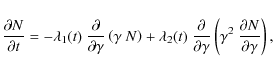
where
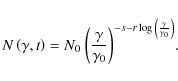
The Fokker-Planck Eq. (B.1) describes the evolution of the electron distribution function; with an initially mono-energetic distribution in the form of a delta-function
![]() (n is the initial particle number density) the solution at subsequent times t takes the form of the log-parabolic energy distribution assumed in Eq. (3) of the main text (see also A.1), reading
(n is the initial particle number density) the solution at subsequent times t takes the form of the log-parabolic energy distribution assumed in Eq. (3) of the main text (see also A.1), reading
Here the time depending slope at
 |
(B.3) |
meanwhile, the curvature of
 |
(B.4) |
from the large initial values corresponding to the initially mono-energetic distribution. Correspondingly, the time-dependent height at
![\begin{displaymath}N_0=\frac{1}{2\sqrt{\pi}}\frac{n}{\gamma_0}\frac{1} {\sqrt{\i...
...mbda_2}}\right)}^2}
{4\int{{\rm d}t~\lambda_2}}}\right]}}\cdot
\end{displaymath}](/articles/aa/full_html/2009/36/aa12237-09/img250.png) |
(B.5) |
To wit, Eq. (B.2) describes the evolution of the electron distribution, growing broader and broader under the effect of stochastic acceleration, while its peak moves from
 |
(B.6) |
under the contrasting actions of the systematic and stochastic accelerations. An important quantity to focus on for the emission properties is the rms energy
| |
 |
||
| = | (B.7) |
which is also the position for the peak of the distribution
We have already derived in Appendix A the shapes of the spectra (synchrotron, and IC in both the Thomson and KN regimes) emitted by the distribution given in Eq. (3); here we stress the time dependence of their main spectral features. We can write for the synchrotron emission![]()
for IC emission we have in the Thomson regime
 |
(B.9) |
and in the extreme KN regime
Note that during flares, since
Now we focus the above relations for the simple case of time independent ![]() and
and ![]() ,
when
,
when
![]() ;
then we have
;
then we have
while for the rms energy we have
so for the peak frequency and the spectral curvature we have
where
The value of ![]() can be evaluated from observing the synchrotron spectral curvatures b2 and b1 at two times t2 and t1, respectively (recall that
can be evaluated from observing the synchrotron spectral curvatures b2 and b1 at two times t2 and t1, respectively (recall that
![]() ); denoting with t2 - t1 this time interval, we have
); denoting with t2 - t1 this time interval, we have
 |
(B.14) |
on the other hand, form observing the related synchrotron peaks
![\begin{displaymath}\lambda_1=\left[{\frac{1}{2\left({t_2 - t_1}\right)}\ln{\left...
...{1}{r_2}-\frac{1}{r_1}}\right)}\right] \frac{1+z}{\delta}\cdot
\end{displaymath}](/articles/aa/full_html/2009/36/aa12237-09/img271.png) |
(B.15) |
For example, in the case of Mrk 501 in the states of 7 and 16 April 1997, we obtain (on assuming
If the total energy available to the jet is limited (e.g., by the BZ limit, see text) we expect that
![]() and
and
![]() cannot grow indefinitely, but are to attain a limiting value. At low energies where
cannot grow indefinitely, but are to attain a limiting value. At low energies where
![]() holds, we have
holds, we have
![]() and
and
![]() as before; at higher energies when
as before; at higher energies when
![]() reaches its limit,
reaches its limit,
![]() holds, leading to
holds, leading to
![]() and
and
![]() .
Eventually also
.
Eventually also
![]() reaches its limit, and both the fluxes and the peak frequencies cannot grow any more.
reaches its limit, and both the fluxes and the peak frequencies cannot grow any more.
Appendix C: Prefactors for Eqs. (4)-(13)
The HSZ SSC model is, as stated before, characterized by five parameters: the rms particle energy
![]() ,
the particle density n, the magnetic field B, the size of the emitting region R and the beaming factor
,
the particle density n, the magnetic field B, the size of the emitting region R and the beaming factor ![]() .
So the model may be constrained by five observables that we denote with
.
So the model may be constrained by five observables that we denote with
 |
(C.1) |
 |
(C.2) |
where the indexes i,j,k,h express the normalizations demonstrated below; in addition, we denote with
In the Thomson regime we find
| B | = | ||
| (C.3) | |||
| = | 13.5 | ||
| (C.4) | |||
| R | = | ||
| (C.5) | |||
| n | = | ||
| (C.6) | |||
| = | (C.7) |
For the extreme KN regime we obtain
| B | = | ||
| (C.8) | |||
| = | |||
| (C.9) | |||
| R | = | ||
| (C.10) | |||
| n | = | ||
| (C.11) | |||
| = | |||
| (C.12) |
Footnotes
- ... tether
- Appendices are only available in electronic form at http://www.aanda.org
- ...Donnarumma et al. 2009)
- The log-parabolic particle energy distribution could be made asymmetric by adding a powerlaw tail at low energies (see Massaro et al. 2006) to represent also low frequency data, e.g., radio in addition to optical/X-ray data; however, here we will focus on the SEDs around their peaks and so we do not use such additions.
- ... density
- Note that in Thomson regime no direct relation appears between electrons emitting peak synchrotron photons and those responsible of IC peak radiation (see Tavecchio et al. 1998).
- ... emission
- Note that singular behaviors of S and C for t=0 are a consequence of the (differential) definition of the SED as
 ,
and relate to the initial singularity of the particle energy distribution. Integrated quantities like
,
and relate to the initial singularity of the particle energy distribution. Integrated quantities like
 behave regularly.
All Tables
Table 1: Source parameters for some BL Lac sources.
Table 2:
Spectral correlations (for
![]() ). We have denoted with
). We have denoted with
![]() or (B) the variations driven by increases of rms electron energy or magnetic field, respectively.
or (B) the variations driven by increases of rms electron energy or magnetic field, respectively.
All Figures
| |
Figure 1:
Two examples of exact, steady SEDs provided by numerical simulations (code by Massaro 2007) after the HSZ SSC model from relativistic electrons with a log-parabolic energy distribution
|
| Open with DEXTER | |
| In the text | |
| |
Figure 2: To illustrate the differences of the IC SEDs in the Thomson and in the extreme KN regime, we show the results of numerical simulations (code by Massaro 2007) after the HSZ SSC model, for different sources with larger and larger rms energy of the radiating particles and other parameters kept constant (including the curvature of the particle energy distribution). The vertical line indicates the frequency of the synchrotron peak where the IC scattering changes over the Thomson to the KN regime (see Eq. (14)). Actual sources in their evolution (represented in Figs. B.1 and B.2) vary their spectral curvature somewhat and only span a limited range in frequency and flux to the left (LBLs) or to the right (HBLs) of the line, with only the IBLs likely to cross it. |
| Open with DEXTER | |
| In the text | |
| |
Figure 3:
Computed changes of spectral parameters corresponding to extended increase of rms particle energy with the other source parameters kept constant. As functions of
|
| Open with DEXTER | |
| In the text | |
| |
Figure 4: As in Fig. 2, we show SEDs obtained from numerical simulations (code by Massaro 2007) of HSZ SSC radiations, for different sources with larger and larger magnetic field B and other parameters kept constant. The vertical line again indicates the transition frequency from the Thomson to the KN regime (see Eq. (15)); as B increases, the IC scattering changes its regime, and reduced cross section yields similar compression effects as in Fig. 2. |
| Open with DEXTER | |
| In the text | |
| |
Figure 5:
Computed changes of spectral parameters as driven by an extended increase of the magnetic field with the other source parameters kept constant. The black full line represents the value of the ratio
|
| Open with DEXTER | |
| In the text | |
| |
Figure 6: Spectral fit of two different states of the IBL source 0716+714. The low state (blue line) data are relative to 1996 November 14 simultaneous observation by AIT, BeppoSAX and EGRET; the high state (red line) data are relative to 2007 September 7-12 simultaneous observations by GASP-WEBT and AGILE-GRID (Tagliaferri et al. 2003; Chen et al. 2008). |
| Open with DEXTER | |
| In the text | |
| |
Figure B.1:
Example of time evolution of the
|
| Open with DEXTER | |
| In the text | |
| |
Figure B.2:
Example of time evolution of the
|
| Open with DEXTER | |
| In the text | |
Copyright ESO 2009
Current usage metrics show cumulative count of Article Views (full-text article views including HTML views, PDF and ePub downloads, according to the available data) and Abstracts Views on Vision4Press platform.
Data correspond to usage on the plateform after 2015. The current usage metrics is available 48-96 hours after online publication and is updated daily on week days.
Initial download of the metrics may take a while.