| Issue |
A&A
Volume 503, Number 2, August IV 2009
|
|
|---|---|---|
| Page(s) | 613 - 624 | |
| Section | Planets and planetary systems | |
| DOI | https://doi.org/10.1051/0004-6361/200911859 | |
| Published online | 02 July 2009 | |
Online Material
Table 8:
Individual spectra. r is the heliocentric distance in astronomical units (AU), ![]() the geocentric distance, Spectro the spectrograph used,
the geocentric distance, Spectro the spectrograph used,
![]() the Modified Julian Day, Run the run number, Exp the exposure time in seconds, R the spectral resolution. Slit and Offset give the size of the entrance slit of the spectrograph and the offset from the nucleus. T and Q are the parameters used for the collisional effects in the synthetic spectra.
the Modified Julian Day, Run the run number, Exp the exposure time in seconds, R the spectral resolution. Slit and Offset give the size of the entrance slit of the spectrograph and the offset from the nucleus. T and Q are the parameters used for the collisional effects in the synthetic spectra.
Appendix A: Estimating the isotopic ratios
Because of uncertainties in the models and systematic errors in the observations, the parameters ![]() and
and ![]() (Eq. (5)) cannot be estimated directly. Additional parameters are required to deal with the exact central wavelength of the lines, and the exact level
of a possible residual background
(Eq. (5)) cannot be estimated directly. Additional parameters are required to deal with the exact central wavelength of the lines, and the exact level
of a possible residual background
![]() .
.
The spectra are divided into small domains surrounding the central wavelength ![]() of the most intense, unblended R lines of 13C14N and 12C15N, i.e., regions where
of the most intense, unblended R lines of 13C14N and 12C15N, i.e., regions where
![]() or
or
![]() .
This is necessary because the accuracy of the 12C14N model is not perfect, especially in the wings of intense lines. Lines of other molecules must also be avoided, e.g., an unidentified feature at
.
This is necessary because the accuracy of the 12C14N model is not perfect, especially in the wings of intense lines. Lines of other molecules must also be avoided, e.g., an unidentified feature at
![]() Å precludes the use of the R10 line of 12C15N close to the nucleus (see Sect. 7).
Å precludes the use of the R10 line of 12C15N close to the nucleus (see Sect. 7).
The line profile of the strongest lines can be fitted by a Gaussian, or their intensity can be estimated by direct integration, providing sets of ![]() and
and ![]() which can then be averaged.
which can then be averaged.
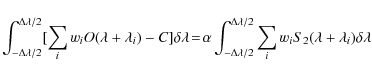
However, in order to reduce the number of free parameters, we used a different procedure. Instead of fitting separately
![]() over the intervals
over the intervals
![]() ,
we superimpose the profiles by shifting the line centers to
,
we superimpose the profiles by shifting the line centers to ![]() ,
optimally coadd them, and fit the resulting profile over the resulting domain
,
optimally coadd them, and fit the resulting profile over the resulting domain
![]() (see Fig. A.1). Hence,
dropping the subscript k, we write, for the 13C14N lines,
(see Fig. A.1). Hence,
dropping the subscript k, we write, for the 13C14N lines,
![\begin{displaymath}%
\sum_i w_i [O(\lambda+\lambda_i) \!-\! C_i]
\!\equiv\!\sum_...
...mbda_i) \!-\! C
\!=\!\alpha \sum_i w_i S_2(\lambda+\lambda_i)~
\end{displaymath}](/articles/aa/olm/2009/32/aa11859-09/img157.png)
and the corresponding formula with S3 and
The width of the observed ``coadded'' profile
![]() is found to be equal to that of the synthetic profile
is found to be equal to that of the synthetic profile
![]() (or
(or
![]() )
and it is symmetric about zero. This confirms that the identification of the 13C14N and 12C15N lines is correct, as well as the theoretical wavelengths adopted for them.
)
and it is symmetric about zero. This confirms that the identification of the 13C14N and 12C15N lines is correct, as well as the theoretical wavelengths adopted for them.
The analysis is done either by profile fitting around ![]() or by direct integration. In the latter case we write
or by direct integration. In the latter case we write
for the 13C14N lines, and an equivalent formula for the 12C15N lines.
The choice of the lines i depends on the quality of the spectra and on particular circumstances, especially the heliocentric distance. Figures 3 and 4 shows that the width of the envelope of the CN band decreases at large r. The relative intensity of the lines of high quantum number drops rapidly. Many lines could be used efficiently for the coadded profiles of comets de Vico or X5 (Fig. A.1), up to 11 for 12C15N and 8 for 13C14N. On the contrary, at large r, a few lines dominate overwhelmingly. As shown in Sect. 7, some blends may become less troublesome far from the nucleus.
![\begin{figure}
\par\includegraphics[angle=-90,width=8.2cm,clip]{11859_11.eps}
\end{figure}](/articles/aa/olm/2009/32/aa11859-09/img164.png) |
Figure A.1: Coadded observed (solid line) and synthetic (with and without the rare isotopologues) spectra of comet C/2002 X5 (Kudo-Fujikawa). The upper panel is centered on 13C14N lines (in this instance, R1-R6, R14 and R16), the lower one on 12C15N lines (R1-R5, R11-R13, R15-R17). The large number of useable isotopic lines is allowed by the good quality of the spectra used in the combination. Intensity is in arbitrary units. |
| Open with DEXTER | |
R lines of 13C14N and 12C15N with low quantum numbers are slightly blended and also - depending on the spectral resolution - with the corresponding R line of 12C14N. An additional difficulty is the presence of faint lines of the B-X (0-0) band of CH. This region of the spectrum needs special care (e.g., some iterative procedure) and may have to be ignored for the lowest quality spectra.
Appendix B: Averages
While weighted averages of measurements xi with errors ei (
![]() )
are easily defined as
)
are easily defined as
![]() ,
estimating the resulting error on this value is less obvious. The global data set is far from homogeneous. Systematic errors affect the various data sets in different ways. The instrumentation and the circumstances are never identical.
Two estimates of the standard error S are sometimes used:
,
estimating the resulting error on this value is less obvious. The global data set is far from homogeneous. Systematic errors affect the various data sets in different ways. The instrumentation and the circumstances are never identical.
Two estimates of the standard error S are sometimes used:
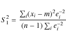
and

They are not satisfying, particularly for a small data set. Equation (B.1) does not take properly into account the individual errors, except for the weighting factors, so that a few xi with large ei but grouped by chance around m would give an unrealistically small S1. On the other hand Eq. (B.2) does not take into account the inter-group variations which can be large in the case of systematic effects. The larger of S1 and S2 may be taken, but we choose a different approach by simulating the xi as the average of ni individual observations yi,j (
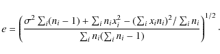
For large
Appendix C: Spectra
![\begin{figure}
\par\includegraphics[angle=270,width=14cm,clip]{11859_12.eps}
\end{figure}](/articles/aa/olm/2009/32/aa11859-09/img175.png) |
Figure C.1: Observed (2DCoudé) and synthetic (dotted) spectra of comet 122P/de Vico. In this and the following graphs, the upper (red) ticks indicate the position of the major R lines of 13C14N the lower (blue) ticks indicate the position of the major R lines of 12C15N. The corresponding quantum numbers are indicated in the upper panel midway between the strong 12C14N lines and the faint isotopic lines. The intensity scale is in relative units. |
| Open with DEXTER | |
![\begin{figure}
\par\includegraphics[angle=270,width=14cm,clip]{11859_13.eps}
\end{figure}](/articles/aa/olm/2009/32/aa11859-09/img176.png) |
Figure C.2: Observed (2DCoudé) and synthetic (dotted) spectra of comet C/1996 B2 (Hyakutake). |
| Open with DEXTER | |
![\begin{figure}
\par\includegraphics[angle=270,width=14cm,clip]{11859_14.eps}
\end{figure}](/articles/aa/olm/2009/32/aa11859-09/img177.png) |
Figure C.3: Observed (2DCoudé) and synthetic (dotted) spectra of comet C/1996 B2 (Hyakutake). |
| Open with DEXTER | |
![\begin{figure}
\par\includegraphics[angle=270,width=14cm,clip]{11859_15.eps}
\end{figure}](/articles/aa/olm/2009/32/aa11859-09/img178.png) |
Figure C.4: Observed (2DCoudé) and synthetic (dotted) spectra of comet C/1995 O1 (Hale-Bopp). |
| Open with DEXTER | |
![\begin{figure}
\par\includegraphics[angle=270,width=14cm,clip]{11859_16.eps}
\end{figure}](/articles/aa/olm/2009/32/aa11859-09/img179.png) |
Figure C.5: Observed (2DCoudé) and synthetic (dotted) spectra of comet C/1995 O1 (Hale-Bopp). |
| Open with DEXTER | |
![\begin{figure}
\par\includegraphics[angle=270,width=14cm,clip]{11859_17.eps}
\end{figure}](/articles/aa/olm/2009/32/aa11859-09/img180.png) |
Figure C.6: Observed (SOFIN) and synthetic (dotted) spectra of comet C/1995 O1 (Hale-Bopp). |
| Open with DEXTER | |
![\begin{figure}
\par\includegraphics[angle=270,width=14cm,clip]{11859_18.eps}
\end{figure}](/articles/aa/olm/2009/32/aa11859-09/img181.png) |
Figure C.7: Observed (2DCoudé) and synthetic (dotted) spectra of comet 55P/Tempel-Tuttle. |
| Open with DEXTER | |
![\begin{figure}
\par\includegraphics[angle=270,width=14cm,clip]{11859_19.eps}
\end{figure}](/articles/aa/olm/2009/32/aa11859-09/img182.png) |
Figure C.8: Observed (2DCoudé) and synthetic (dotted) spectra of comet C/1999 H1 (Lee). |
| Open with DEXTER | |
![\begin{figure}
\par\includegraphics[angle=270,width=14cm,clip]{11859_20.eps}
\end{figure}](/articles/aa/olm/2009/32/aa11859-09/img183.png) |
Figure C.9: Observed (2DCoudé) and synthetic (dotted) spectra of comet C/1999 S4 (LINEAR). |
| Open with DEXTER | |
![\begin{figure}
\par\includegraphics[angle=270,width=14cm,clip]{11859_21.eps}
\end{figure}](/articles/aa/olm/2009/32/aa11859-09/img184.png) |
Figure C.10: Observed (2DCoudé) and synthetic (dotted) spectra of comet C/1999 T1 (McNaught-Hartley). |
| Open with DEXTER | |
![\begin{figure}
\par\includegraphics[angle=270,width=14cm,clip]{11859_22.eps}
\end{figure}](/articles/aa/olm/2009/32/aa11859-09/img185.png) |
Figure C.11: Observed (2DCoudé) and synthetic (dotted) spectra of comet C/2001 A2-A (LINEAR). |
| Open with DEXTER | |
![\begin{figure}
\par\includegraphics[angle=270,width=14cm,clip]{11859_23.eps}
\end{figure}](/articles/aa/olm/2009/32/aa11859-09/img186.png) |
Figure C.12: Observed (UVES) and synthetic (dotted) spectra of comet C/2000 WM1 (LINEAR). |
| Open with DEXTER | |
![\begin{figure}
\par\includegraphics[angle=270,width=14cm,clip]{11859_24.eps}
\end{figure}](/articles/aa/olm/2009/32/aa11859-09/img187.png) |
Figure C.13: Observed (2DCoudé) and synthetic (dotted) spectra of comet 153P/Ikeya-Zhang. |
| Open with DEXTER | |
![\begin{figure}
\par\includegraphics[angle=270,width=14cm,clip]{11859_25.eps}
\end{figure}](/articles/aa/olm/2009/32/aa11859-09/img188.png) |
Figure C.14: Observed (UVES) and synthetic (dotted) spectra of comet C/2002 X5 (Kudo-Fujikawa). |
| Open with DEXTER | |
![\begin{figure}
\par\includegraphics[angle=270,width=14cm,clip]{11859_26.eps}
\end{figure}](/articles/aa/olm/2009/32/aa11859-09/img189.png) |
Figure C.15: Observed (UVES) and synthetic (dotted) spectra of comet C/2002 V1 (NEAT). |
| Open with DEXTER | |
![\begin{figure}
\par\includegraphics[angle=270,width=14cm,clip]{11859_27.eps}
\end{figure}](/articles/aa/olm/2009/32/aa11859-09/img190.png) |
Figure C.16: Observed (UVES) and synthetic (dotted) spectra of comet C/2002 Y1 (Juels-Holvorcem). |
| Open with DEXTER | |
![\begin{figure}
\par\includegraphics[angle=270,width=14cm,clip]{11859_28.eps}
\end{figure}](/articles/aa/olm/2009/32/aa11859-09/img191.png) |
Figure C.17: Observed (UVES) and synthetic (dotted) spectra of comet 88P/Howell. |
| Open with DEXTER | |
![\begin{figure}
\par\includegraphics[angle=270,width=14cm,clip]{11859_29.eps}
\end{figure}](/articles/aa/olm/2009/32/aa11859-09/img192.png) |
Figure C.18: Observed (UVES) and synthetic (dotted) spectra of comet C/2002 T7 (LINEAR). |
| Open with DEXTER | |
![\begin{figure}
\par\includegraphics[angle=270,width=14cm,clip]{11859_30.eps}
\end{figure}](/articles/aa/olm/2009/32/aa11859-09/img193.png) |
Figure C.19: Observed (UVES) and synthetic (dotted) spectra of comet C/2001 Q4 (NEAT). |
| Open with DEXTER | |
![\begin{figure}
\par\includegraphics[angle=270,width=14cm,clip]{11859_31.eps}
\end{figure}](/articles/aa/olm/2009/32/aa11859-09/img194.png) |
Figure C.20: Observed (UVES) and synthetic (dotted) spectra of comet C/2001 Q4 (NEAT). |
| Open with DEXTER | |
![\begin{figure}
\par\includegraphics[angle=270,width=14cm,clip]{11859_32.eps}
\end{figure}](/articles/aa/olm/2009/32/aa11859-09/img195.png) |
Figure C.21: Observed (UVES) and synthetic (dotted) spectra of comet C/2003 K4 (LINEAR). |
| Open with DEXTER | |
![\begin{figure}
\par\includegraphics[angle=270,width=14cm,clip]{11859_33.eps}
\end{figure}](/articles/aa/olm/2009/32/aa11859-09/img196.png) |
Figure C.22: Observed (UVES) and synthetic (dotted) spectra of comet C/2003 K4 (LINEAR). |
| Open with DEXTER | |
![\begin{figure}
\par\includegraphics[angle=270,width=14cm,clip]{11859_34.eps}
\end{figure}](/articles/aa/olm/2009/32/aa11859-09/img197.png) |
Figure C.23: Observed (HIRES) and synthetic (dotted) spectra of comet 9P/Tempel 1. |
| Open with DEXTER | |
![\begin{figure}
\par\includegraphics[angle=270,width=14cm,clip]{11859_35.eps}
\end{figure}](/articles/aa/olm/2009/32/aa11859-09/img198.png) |
Figure C.24: Observed (UVES) and synthetic (dotted) spectra of comet 9P/Tempel 1. |
| Open with DEXTER | |
![\begin{figure}
\par\includegraphics[angle=270,width=14cm,clip]{11859_36.eps}
\end{figure}](/articles/aa/olm/2009/32/aa11859-09/img199.png) |
Figure C.25: Observed (UVES) and synthetic (dotted) spectra of comet 73P-B/Schwassmann-Wachmann 3. |
| Open with DEXTER | |
![\begin{figure}
\par\includegraphics[angle=270,width=14cm,clip]{11859_37.eps}
\end{figure}](/articles/aa/olm/2009/32/aa11859-09/img200.png) |
Figure C.26: Observed (2DCoudé) and synthetic (dotted) spectra of comet 73P-B/Schwassmann-Wachmann 3. |
| Open with DEXTER | |
![\begin{figure}
\par\includegraphics[angle=270,width=14cm,clip]{11859_38.eps}
\end{figure}](/articles/aa/olm/2009/32/aa11859-09/img201.png) |
Figure C.27: Observed (UVES) and synthetic (dotted) spectra of comet 73P-C/Schwassmann-Wachmann 3. |
| Open with DEXTER | |
![\begin{figure}
\par\includegraphics[angle=270,width=14cm,clip]{11859_39.eps}
\end{figure}](/articles/aa/olm/2009/32/aa11859-09/img202.png) |
Figure C.28: Observed (2DCoudé) and synthetic (dotted) spectra of comet 73P-C/Schwassmann-Wachmann 3. |
| Open with DEXTER | |
![\begin{figure}
\par\includegraphics[angle=270,width=14cm,clip]{11859_40.eps}
\end{figure}](/articles/aa/olm/2009/32/aa11859-09/img203.png) |
Figure C.29: Observed (2DCoudé) and synthetic (dotted) spectra of comet C/2006 M4 (SWAN). |
| Open with DEXTER | |
![\begin{figure}
\par\includegraphics[angle=270,width=14cm,clip]{11859_41.eps}
\end{figure}](/articles/aa/olm/2009/32/aa11859-09/img204.png) |
Figure C.30: Observed (HIRES) and synthetic (dotted) spectra of comet 17P/Holmes. |
| Open with DEXTER | |
![\begin{figure}
\par\includegraphics[angle=270,width=14cm,clip]{11859_42.eps}
\end{figure}](/articles/aa/olm/2009/32/aa11859-09/img205.png) |
Figure C.31: Observed (2DCoudé) and synthetic (dotted) spectra of comet 17P/Holmes. |
| Open with DEXTER | |
![\begin{figure}
\par\includegraphics[angle=270,width=14cm,clip]{11859_43.eps}
\end{figure}](/articles/aa/olm/2009/32/aa11859-09/img206.png) |
Figure C.32: Observed (2DCoudé) and synthetic (dotted) spectra of comet 8P/Tuttle. |
| Open with DEXTER | |
![\begin{figure}
\par\includegraphics[angle=270,width=14cm,clip]{11859_44.eps}
\end{figure}](/articles/aa/olm/2009/32/aa11859-09/img207.png) |
Figure C.33: Observed (2DCoudé) and synthetic (dotted) spectra of comet C/2007 N3 (Lulin). |
| Open with DEXTER | |
D Synthetic spectra
![\begin{figure}
\par\includegraphics[width=8.5cm,clip]{11859_45.eps}
\end{figure}](/articles/aa/olm/2009/32/aa11859-09/img208.png) |
Figure D.1:
Small region of the B-X 0-0 band of the three CN isotopologues.
The synthetic spectra were computed using isotopic abundances of 1, 1/89 and 1/145 for 12C14N (black), 13C14N (red) and 12C15N (blue), respectively, in the absence of collisional effects, and with r=1 AU, |
| Open with DEXTER | |
![\begin{figure}
\par\includegraphics[width=8.5cm,clip]{11859_46.eps}
\end{figure}](/articles/aa/olm/2009/32/aa11859-09/img209.png) |
Figure D.2: Same as Fig. D.1 for a region of the B-X 0-1 band. |
| Open with DEXTER | |
![\begin{figure}
\par\includegraphics[width=8.5cm,clip]{11859_47.eps}
\end{figure}](/articles/aa/olm/2009/32/aa11859-09/img210.png) |
Figure D.3: Same as Fig. D.1 for a region of the A-X 2-0 band. |
| Open with DEXTER | |
![\begin{figure}
\includegraphics[width=8.5cm,clip]{11859_48.eps}
\end{figure}](/articles/aa/olm/2009/32/aa11859-09/img211.png) |
Figure D.4: Same as Fig. D.1 for a region of the A-X 1-0 band. |
| Open with DEXTER | |
Current usage metrics show cumulative count of Article Views (full-text article views including HTML views, PDF and ePub downloads, according to the available data) and Abstracts Views on Vision4Press platform.
Data correspond to usage on the plateform after 2015. The current usage metrics is available 48-96 hours after online publication and is updated daily on week days.
Initial download of the metrics may take a while.