| Issue |
A&A
Volume 503, Number 2, August IV 2009
|
|
|---|---|---|
| Page(s) | 613 - 624 | |
| Section | Planets and planetary systems | |
| DOI | https://doi.org/10.1051/0004-6361/200911859 | |
| Published online | 02 July 2009 | |
The CN isotopic ratios in comets![[*]](/icons/foot_motif.png) ,
,
J. Manfroid1,![]() -
E. Jehin1,
-
E. Jehin1,![]() -
D. Hutsemékers1,
-
D. Hutsemékers1,![]() -
A. Cochran2 -
J.-M. Zucconi3,
-
A. Cochran2 -
J.-M. Zucconi3,![]() - C. Arpigny1 -
R. Schulz4 -
J. A. Stüwe5 -
I. Ilyin6
- C. Arpigny1 -
R. Schulz4 -
J. A. Stüwe5 -
I. Ilyin6
1 - Institut d'Astrophysique et de Géophysique, Université de Liège, Allée du 6 août 17, 4000 Liège, Belgium
2 -
Department of Astronomy and McDonald Observatory, University of Texas at Austin, C-1400, Austin, USA
3 -
Observatoire de Besançon, 25010 Besançon Cedex, France
4 -
ESA/RSSD, ESTEC, PO Box 299, NL-2200 AG Noordwijk, The Netherlands
5 -
Leiden Observatory, 2300 RA Leiden, The Netherlands
6 -
AIP, An der Sternwarte 16, 14482 Potsdam, Germany
Received 17 February 2009 / Accepted 9 June 2009
Abstract
Our aim is to determine the isotopic ratios 12C/13C and 14N/15N in a variety of comets and link these measurements to the formation and evolution of the solar
system. The 12C/13C and 14N/15N isotopic ratios are measured for the CN radical
by means of high-resolution optical spectra of the R branch of the B-X (0, 0) violet band. 23 comets from different dynamical classes have been observed, sometimes at various heliocentric
and nucleocentric distances, in order to estimate possible variations of the isotopic ratios in parent molecules. The 12C/13C and 14N/15N isotopic ratios in CN are remarkably constant (average values of, respectively, 91.0 ![]() 3.6 and 147.8
3.6 and 147.8 ![]() 5.7) within our measurement errors, for all comets whatever their origin or heliocentric distance. While the carbon isotopic ratio does agree with the terrestrial value (89), the nitrogen ratio is a factor of two lower than the terrestrial value (272), indicating a fractionation in the early solar system,
or in the protosolar nebula, common to all the comets of our sample. This points towards a common
origin of the comets independently of their birthplaces, and a relationship between HCN and CN.
5.7) within our measurement errors, for all comets whatever their origin or heliocentric distance. While the carbon isotopic ratio does agree with the terrestrial value (89), the nitrogen ratio is a factor of two lower than the terrestrial value (272), indicating a fractionation in the early solar system,
or in the protosolar nebula, common to all the comets of our sample. This points towards a common
origin of the comets independently of their birthplaces, and a relationship between HCN and CN.
Key words: comets: general - techniques: spectroscopic - line: identification - line: profiles - molecular processes
1 Introduction
Comets are believed to have condensed in the outer solar nebula and to contain relatively unaltered material from that period. The analysis of the composition of such material and particularly the determination of isotopic ratios should answer questions regarding the origin and the nature of the solar nebula.
This task is challenging. In-situ measurements in the coma with mass spectrometers are difficult, because heavy isotopes can be masked by hydrides, e.g., 13C and 12CH, 15N and 14NH. Values exist from in-situ measurements for the dust coma of comet 1P/Halley, for which the carbon isotopic ratio, 12C/13C, varied by orders of magnitude from one grain to another (Solc et al. 1987; Jessberger & Kissel 1991) - but no data were available for nitrogen.
Isotopic ratios can be determined remotely by high-resolution spectroscopy of molecular bands. The emission lines of rare isotopes are weak and they have to be distinguished from emission lines of other isotopes, other species (e.g., NH2 in the case of the C2 Swan bands) and from the background. Likewise, blends are possible at sub-millimetre range: e.g., SO2 blends with the H13CN (4-3) line (Lis et al. 1997a). Hence, high spectral resolution and high signal-to-noise ratios are needed. The accuracy of these determinations also depends on the models representing the emission by the various isotopologues, as well as other species appearing in the same domain.
Up to now, isotopic ratios have been published for H, C, N, O and S (Jehin et al. 2006). The Rosetta mission to 67P/Churyumov-Gerasimenko will provide a detailed appraisal of the nature and isotopic composition of the material present at the surface of one comet. The present work addresses the C and N ground-based determinations that can now be routinely obtained for moderately bright comets.
2 Historical background
For carbon and nitrogen isotopes, the first observed molecules were CN and C2 in the optical and HCN in the sub-millimetre range. The first determinations of the 12C/13C ratio were obtained for bright comets from the 12C13C (1, 0) Swan bandhead at 4145 Å (Stawikowski & Greenstein 1964; Owen 1973). This feature was chosen because it is clearly separated from the corresponding 12C12C bandhead. However, these measurements were affected by blending with NH2 emission. The cleaner CN B-X (0-0) band was used for the first time for comet 1P/Halley (Wyckoff & Wehinger 1988; Wyckoff et al. 1989; Kleine et al. 1995), resulting in positive determinations of 12C/13C. By 2000, estimates of the 12C/13C ratio were available for ten comets. Although the same CN band lends itself to the determination of the nitrogen ratio, only lower limits were obtained.
The nitrogen isotopic ratio 14N/15N was measured for the first time in comet C/1995 O1 (Hale-Bopp) in 1997 in the HCN as well as the CN band. The 12C/13C ratio was determined simultaneously. The 12C/13C and 14N/15N values derived from the HCN band at sub-millimetre range (respectively 111 ![]() 12 and 323
12 and 323 ![]() 46, Jewitt et al. 1997; 109
46, Jewitt et al. 1997; 109 ![]() 22 and 330
22 and 330 ![]() 98, Ziurys et al. 1999), were consistent with the telluric values (89, 272, Anders & Grevesse 1989), although with large
uncertainties. The 12C/13C values derived from CN (12C/13C = 100
98, Ziurys et al. 1999), were consistent with the telluric values (89, 272, Anders & Grevesse 1989), although with large
uncertainties. The 12C/13C values derived from CN (12C/13C = 100 ![]() 35) were terrestrial, but the nitrogen isotopic ratio (14N/15N = 140
35) were terrestrial, but the nitrogen isotopic ratio (14N/15N = 140 ![]() 35) was widely discordant with the terrestrial and HCN values (Arpigny et al. 2000, 2003).
35) was widely discordant with the terrestrial and HCN values (Arpigny et al. 2000, 2003).
Examination of published spectra of several other bright comets showed that 12C15N was probably also overabundant. The unexpected strength of these lines was a reason for discarding them as 12C15N (see, e.g., features labelled k, m and o in the Halley spectrum displayed in Fig. 5 of Kleine et al. 1995, or lines c and d in the C/1990 K1 spectrum in Fig. 8 of Wyckoff et al. 2000).
This discrepancy between CN and HCN, a presumed parent, was eventually solved with the observation of CN and HCN in comet 17P/Holmes and the reanalysis of the Hale-Bopp sub-millimeter data (Bockelée-Morvan et al. 2008a) establishing that HCN has the same non-terrestrial nitrogen isotopic composition as CN.
The seemingly conflicting results and the evidence for an anomalous value of 14N/15N had led us to initiate an observing campaign with the UVES high-resolution spectrograph (Dekker et al. 2000) mounted on the 8 m Kueyen telescope of the ESO VLT (Chile), in order to gather data on different comets presenting a variety of origins and physical conditions. The CN
![]() (0, 0) violet band (near 3880 Å) was our main target.
(0, 0) violet band (near 3880 Å) was our main target.
Independently, in the Northern hemisphere, observations of many comets have been made since 1995 with the 2DCoudé high-resolution spectrograph of the 2.7 m telescope of the McDonald Observatory (Tull et al. 1995) and contributed a large proportion of our CN data.
3 Our sample of comets and previous results
So far, 23 comets have been observed (counting the fragments of 73P/Schwassmann-Wachmann 3 as one comet). They are listed in Table 2, with basic orbital characteristics including the Tisserand parameter ![]() relative to Jupiter:
relative to Jupiter:
 |
(1) |
a and
Our sample does not contain Levison's Encke-type objects (defined as
![]() ,
,
![]() ).
Considering Horner's classification, SP
).
Considering Horner's classification, SP![]() is missing and SP
is missing and SP
![]() is barely realized by the fragments of 73P/SW-3. The sample shows a majority of the long period objects (according to Horner's scheme) divided equally in external and new comets (Levison's scheme). There are two comets from the Halley family (SP
is barely realized by the fragments of 73P/SW-3. The sample shows a majority of the long period objects (according to Horner's scheme) divided equally in external and new comets (Levison's scheme). There are two comets from the Halley family (SP![]() )
and four from the Jupiter family (one SP
)
and four from the Jupiter family (one SP
![]() and three SP
and three SP![]() ), considering the two fragments of 73P as a single member.
), considering the two fragments of 73P as a single member.
We could not derive isotopic abundances for all 23 observed comets mainly because of the insufficient signal-to-noise ratio of the CN band, but 18 comets yielded positive measurements of both C and N ratios. Results have already been published partially for 10 of them. Our first target for UVES was comet C/2000 WM1 (LINEAR) which showed isotopic ratios compatible with those we had found in Hale-Bopp (Arpigny et al. 2000). This isotopic anomaly and the discrepancy with the N ratio determined from HCN in comet Hale-Bopp (Jewitt et al. 1997; Ziurys et al. 1999) led us to suggest the existence of parent(s) of CN other than HCN, with an even lower N isotopic ratio. Organic compounds like those found in interplanetary dust particles were proposed as possible candidates (Arpigny et al. 2003).
Our analysis of data gathered at McDonald observatory on 122P/de Vico and 153P/Ikeya-Zhang yielded isotopic ratios similar to Hale-Bopp and C/2000 WM1 (LINEAR) (Jehin et al. 2004).
Most observations were done at small heliocentric distances since this yields the brightest
![]() ,
i.e., the magnitude that would be seen from a distance of 1 AU - a good indication of the flux entering the slit of the spectrometer. However, we gathered data on comets over a wider range of heliocentric distance in the hope of detecting variations of the isotopic ratios linked to
different abundances of the parent species. It is likely that at large distances, the CN radical originates mainly from the photodissociation of HCN (see, e.g., Rauer et al. 2003). The isotopic ratios were determined in comets C/1995 O1 (Hale-Bopp), C/2001 Q4 (NEAT) and C/2003 K4 (LINEAR) at heliocentric distances of, respectively, 2.7, 3.7 and 2.6 AU (Manfroid et al. 2005) as well as close to 1 AU. No significant differences were found as a function of heliocentric distance, and the values were consistent with those obtained for other comets. The apparent discrepancy between the nitrogen isotopic ratio measurements in CN and HCN over such a range of irradiation conditions seemed to rule out HCN as a major parent
of the cometary CN radicals.
,
i.e., the magnitude that would be seen from a distance of 1 AU - a good indication of the flux entering the slit of the spectrometer. However, we gathered data on comets over a wider range of heliocentric distance in the hope of detecting variations of the isotopic ratios linked to
different abundances of the parent species. It is likely that at large distances, the CN radical originates mainly from the photodissociation of HCN (see, e.g., Rauer et al. 2003). The isotopic ratios were determined in comets C/1995 O1 (Hale-Bopp), C/2001 Q4 (NEAT) and C/2003 K4 (LINEAR) at heliocentric distances of, respectively, 2.7, 3.7 and 2.6 AU (Manfroid et al. 2005) as well as close to 1 AU. No significant differences were found as a function of heliocentric distance, and the values were consistent with those obtained for other comets. The apparent discrepancy between the nitrogen isotopic ratio measurements in CN and HCN over such a range of irradiation conditions seemed to rule out HCN as a major parent
of the cometary CN radicals.
The isotopic ratios were then determined for the first time in a Jupiter-family (SP![]() )
comet, 88P/Howell, and in the chemically peculiar Oort Cloud comet C/1999 S4 (LINEAR) (Hutsemékers et al. 2005). The carbon and nitrogen isotopic ratios agreed
within the uncertainties with those already obtained.
)
comet, 88P/Howell, and in the chemically peculiar Oort Cloud comet C/1999 S4 (LINEAR) (Hutsemékers et al. 2005). The carbon and nitrogen isotopic ratios agreed
within the uncertainties with those already obtained.
The Deep Impact mission to comet 9P/Tempel 1 provided an extraordinary opportunity to observe from the ground the cometary material coming from relatively deep (a few meters) layers of the nucleus. The impact resulted in the release of sub-surface material from the comet nucleus (A'Hearn et al. 2005), which formed a jet structure that expanded within the coma and was observable for several days after the impact. Observations of the activity and composition of the comet after the impact showed that the new material was compositionally different from that seen before impact and that the mass ratio of dust to gas in the ejecta was much larger than before (Meech et al. 2005). This suggested that the isotopic abundances could be different too.
Observations of comet 9P/Tempel 1 were carried out before, during, and after the collision with the optical spectrometers UVES and HIRES mounted on the Kueyen telescope of the ESO VLT (Chile) and the Keck I telescope on Mauna Kea (Hawaii), respectively (Jehin et al. 2006). They show that the material released by the impact probably has the same carbon and nitrogen isotopic composition as the surface material, once again in line with the values derived so far.
Whether the material came from layers deep enough to be unaffected by space weathering remains unknown. If indeed the Deep Impact event led to the release of pristine material representative of the unaltered matter preserved in the interior of a comet nucleus since its formation, the measurement of the same isotopic composition in CN before and after impact would provide evidence for the 12C/13C and 14N/15N isotopic ratios being primordial in the parent molecule that produces CN. However, infrared measurements obtained before and after impact showed an enhanced C2H6/H2O ratio, but an unchanged HCN/H2O ratio relative to the quiescent (pre-impact) source (DiSanti & Mumma 2008). It may therefore be that non-altered CN-bearing material had not been reached by the impact. However, the processes that could affect the isotopic ratios are not the same as those affecting the relative amounts of volatiles near the surface. It is also possible that the nucleus is not differentiated in HCN.
The 2007 outburst of the Jupiter Family comet 17P/Holmes allowed us to reconcile the HCN and CN data (Bockelée-Morvan et al. 2008a). Observation of J=3-2 rotational lines of H12C14N, H12C15N and H13C14N yielded 14N/15N = 139 ![]() 26 while the measurements of the CN violet band gave 14N/15N = 165
26 while the measurements of the CN violet band gave 14N/15N = 165 ![]() 40. Moreover it appeared that the HCN ratios that had been published for Hale-Bopp were seriously overestimated. A reanalysis of the data gave 138 < 14N/15N < 239, and 12C/13C = 94
40. Moreover it appeared that the HCN ratios that had been published for Hale-Bopp were seriously overestimated. A reanalysis of the data gave 138 < 14N/15N < 239, and 12C/13C = 94 ![]() 8. The isotopic ratios derived from CN and HCN are thus compatible within the error bars, and in line with those we measured in other comets.
8. The isotopic ratios derived from CN and HCN are thus compatible within the error bars, and in line with those we measured in other comets.
In the following sections, we present a homogeneous compilation of the whole data set and revisit the previous results. Isotopic ratios of 8 comets are given for the first time. This completely new analysis uses, in particular, the latest fluorescence model including a more realistic handling of the collisional effects.
4 Observations
![\begin{figure}
\par\includegraphics[width=8.8cm,clip]{11859_1.eps}
\end{figure}](/articles/aa/full_html/2009/32/aa11859-09/img24.png) |
Figure 1:
Synthetic spectrum of 12C14N over the whole optical domain (r=1 AU, |
| Open with DEXTER | |
In order to study the carbon and nitrogen isotopes in cometary spectra, we chose to observe the (0, 0) violet band (B-X) of CN. Figure 1 shows a typical (synthetic) 12C14N spectrum over the whole optical domain. The spectra of the heavier isotopologues have very similar distributions. The red bands are sparser than the blue ones, so the
actual flux emitted in each band cannot be easily inferred from the figure. They are given in Table 1. Most of the optical emission occurs in the violet (0-0) band at 3880 Å and in the red (
![]() )
bands between 9000 and 10 000 Å.
However, the red spectrum is more dispersed over many more lines.
)
bands between 9000 and 10 000 Å.
However, the red spectrum is more dispersed over many more lines.
Table 1: Relative flux emitted in the various CN bands shown in Fig. 1.
To better appreciate which lines are the most useful, the brightest domains of the spectra of the three species (12C14N, 13C14N and 12C15N) are shown in Figs. D.1-D.4.
Comparison with the atlas of comet de Vico (Cochran & Cochran 2002) shows several of these isotopic lines among the unidentified features.
The B-X (0, 0) band appears to be the most interesting for our purposes. The lines are strong, and at that wavelength the solar spectrum is relatively weak. The red A-X bands are affected by emission from other molecules (mainly NH2 and C2 - see, e.g., the de Vico atlas), a stronger solar background and complex absorption by atmospheric features (H2O, O2). The B-X (0, 1) band at 420 nm is also fainter and, hence, less useful for our purposes. Ideally, all these bands could be included in a global analysis to provide the best estimate of the isotopic ratios as well as the physical parameters in the coma but, in the present work, we limit ourselves to the bright (0-0) violet band.
High-resolution spectra are needed because the faint emission of the rare species are close to the strong lines coming from the abundant ones and because the best contrast to the underlying dust-scattered solar continuum must be obtained. Only the R branch is of interest because the wavelength shifts in the P branch are small compared to the typical spectral resolution and Doppler broadening of the lines.
Table 2: Observed comets.
Table 3: Observational circumstances.
The echelle spectrographs used in the present study were
- The UVES spectrograph at the Nasmyth focus of the 8 m Kueyen telescope (ESO/VLT, Paranal);
- SOFIN, the Cassegrain spectrograph at the 2.56 m NOT telescope (La Palma, Spain);
- the 2dCoudé echelle spectrograph at the 2.7 m Harlan F. Smith telescope of the
McDonald Observatory (Texas);
- the HIRES spectrograph of the 10 m Keck I telescope (Hawaii).
5 Data reduction
We used the echelle package of the IRAF software (NOAO) to calibrate the spectra and to extract the relevant order(s) of the CN violet band. In the case of the VLT spectra, the UVES configuration is such that the CN band appears in two orders. The SOFIN and 2DCoudé spectra do not suffer from the same problem: all of the band is in a single order. The UVES wavelength calibration was done on the CN lines themselves in order to avoid possible shifts between the science spectra and calibration lamp spectra. Indeed, the UVES calibration errors measured between the CN and lamp solutions show an rms scatter of 0.66 km s-1.
The echelle orders were combined using an optimal scheme taking into account the low levels expected for the isotopic lines - i.e., a regime where the signal-to-noise ratio is directly proportional to the signal - and simultaneously correcting the echelle ripple (blaze function). The wavelength domain is very small, ![]() Å, so that a normalization is done in such a way that flat-field spectra extracted in the same conditions are constant. This procedure yields the ``flat-field normalized'' spectrum
Å, so that a normalization is done in such a way that flat-field spectra extracted in the same conditions are constant. This procedure yields the ``flat-field normalized'' spectrum
![]() and the S/N ratio expected for a low-level constant signal,
and the S/N ratio expected for a low-level constant signal,
![]() .
The S/N ratios of faint lines of intensity I can be directly compared using
.
The S/N ratios of faint lines of intensity I can be directly compared using

Alternatively, a ``S/N-normalized'' spectrum
![\begin{figure}
\par\includegraphics[width=8.5cm,clip]{11859_2.eps}
\end{figure}](/articles/aa/full_html/2009/32/aa11859-09/img36.png) |
Figure 2:
Variations of of the signal-to-noise ratio
|
| Open with DEXTER | |
A typical
![]() is presented in Fig. 2. The minimum falls on the CN band, in the overlapping region between two echelle orders, and corresponds approximately to a 2-1/2 loss. Unfortunately, changing the relevant UVES settings so as to bring the CN R band in the middle of one order was not possible.
is presented in Fig. 2. The minimum falls on the CN band, in the overlapping region between two echelle orders, and corresponds approximately to a 2-1/2 loss. Unfortunately, changing the relevant UVES settings so as to bring the CN R band in the middle of one order was not possible.
The dust-reflected sunlight and, in some cases, the twilight contamination and the lunar sky background underlying the cometary emissions, were removed from the
![]() by fitting a solar reference spectrum to each of these components. Moon or twilight sky spectra were often used
for this purpose as they directly provided correct line profiles, but other good high-resolution solar spectra can be used, such as the UVES reference solar spectrum produced by ESO
or the atlas by Delbouille et al. (1973), available online at the BASS2000 site (http://bass2000.obspm.fr/solar_spect.php).
by fitting a solar reference spectrum to each of these components. Moon or twilight sky spectra were often used
for this purpose as they directly provided correct line profiles, but other good high-resolution solar spectra can be used, such as the UVES reference solar spectrum produced by ESO
or the atlas by Delbouille et al. (1973), available online at the BASS2000 site (http://bass2000.obspm.fr/solar_spect.php).
Appropriate Doppler shifts had to be applied since, at the resolution of the echelle spectra, the observer, the Moon, the Sun and the comet have non-negligible relative velocities.
- The Moon spectrum and the lunar sky background show a radial velocity equal to the sum of the heliocentric and topocentric velocities of the Moon;
- the dust-reflected sunlight shows a radial velocity equal to the sum of the heliocentric
and topocentric velocities of the comet;
- the twilight component is shifted by the topocentric velocity of the Sun;
- the cometary emission is shifted by the topocentric velocity of the comet.
The transfer functions (line profiles) of those components are not identical. The profiles of the various solar components were fitted by convolution with a Gaussian kernel. This transformation was generally negligible, except for widely discordant resolution (e.g., some SOFIN spectra of Hale-Bopp with too long exposures at too low elevations in the Cassegrain focus). The intensity fit was done by comparing the intensity of the solar photospheric lines in each component.
After removal of the dust, twilight and moonlight spectra, no solar feature subsists. The remaining contamination consists of an extremely weak quasi-featureless continuum due to a residual of improperly subtracted scattered light in the instrument, and to the underlying sky background. This continuum is fitted by a spline through the emission-free intervals of the spectrum and is subtracted from the spectrum.
The signal levels on the CCD amount at best to only a few electrons per pixel above the bias level, except in the major R lines of the abundant species where it is typically 102 to 103 electrons.
The linearity of the spectrographs is very good, and well maintained. For instance at ESO, the linearity of the UVES detector between 0 and 105 ADU is guaranteed to within about 1% by the frequent verifications performed by the staff. Whenever possible, however, we checked the linearity directly on our data by comparing cometary lines and stellar spectra appearing in overlapping orders with vastly different sensitivities. The comparison of specific line ratios to their theoretical values yields the same conclusion.
![\begin{figure}
\par\includegraphics[width=17cm,clip]{11859_3.eps}
\end{figure}](/articles/aa/full_html/2009/32/aa11859-09/img38.png) |
Figure 3:
Synthetic spectra of 12C14N at various heliocentric distances. The intensity scale is arbitrary. The R-branch of the (0-0) band extends shortward of 3875 Å
and the P-branch longward of 3875 Å. Weak lines of the P-branch of the (1-1) band are visible at wavelengths shorter than 3872.5 Å. The black spectra correspond to a collisionless coma with |
| Open with DEXTER | |
6 Fluorescence model of CN
The structure of the CN radical and the details of the fluorescence calculations are presented elsewhere (Zucconi & Festou 1985) and will not be repeated here. Instead, we will only focus on some features and on their improvements.
The CN fluorescence is very sensitive to the Swings effect (Swings 1941) and the computation requires accurate line wavelengths and solar fluxes. Wavelengths of the 12C14N B-X system (the violet system) have been computed using the spectroscopic constants of Ram et al. (2006), leading to an accuracy better than 1 mÅ. On the other hand we have used the Kurucz atlas (Kurucz 2005) to evaluate the solar intensities in the violet bands.
The influence of the A-X system on the shape of the violet bands cannot be neglected because the pumping via this system also affects the population of the ground state levels.
Unfortunately, we do not have high-resolution absolute spectra of the Sun in the red and near infrared. Ground-based atlases contain many strong water absorption lines and are unsuitable. Hence we decided to use the solar fluxes of Labs & Neckel (1970). Although the Swings effect is thus ignored in the red bands, we obtain a better fit of the spectra than when using the Kurucz atlas in the red and near infrared. This could be due to the fact that there is a large number of CN lines in those bands, minimizing the Swings effect. There is no extensive laboratory study of the violet bands of 13C14N and 12C15N and only the most intense bands have been observed. We derived the isotope line wavelengths from the 12C14N lines using the isotopic shift formula. The predicted wavelengths agree with the faint isotope lines observed in our spectra. We also checked that the computed wavelengths agree with the available data for the ground vibrational state (Hübner et al. 2005).
Dipole moment, radiative lifetimes and Franck-Condon factors for the violet bands are those listed in Zucconi & Festou (1985) and we adjusted the vibrational transition rate and the
lifetime
![]() of the A state to get the best fit of our observations. The value adopted for
of the A state to get the best fit of our observations. The value adopted for
![]()
![]() ,
10-5 s, is very close to the average between various experimental measurements and theoretical estimates (e.g., Lu et al. 1992;
Bauschlicher et al. 1988, and references therein). It is also in excellent agreement with the value based on a recent analysis of the solar spectrum (Sauval et al. 2009).
,
10-5 s, is very close to the average between various experimental measurements and theoretical estimates (e.g., Lu et al. 1992;
Bauschlicher et al. 1988, and references therein). It is also in excellent agreement with the value based on a recent analysis of the solar spectrum (Sauval et al. 2009).
![\begin{figure}
\par\includegraphics[width=17cm,clip]{11859_4.eps}
\end{figure}](/articles/aa/full_html/2009/32/aa11859-09/img41.png) |
Figure 4: Same as Fig. 3 for 12C15N. |
| Open with DEXTER | |
Because we probe the central part of the coma, collisions may play a non negligible role and we had to include this effect in our model. Ideally this would lead to consideration of the density variation in the field of view and the dependence of collisional cross sections as a function of the relative velocity of the colliders and of the rotational quantum number.
The general formula expressing the transition probability between two levels is given by
where u and l denote the upper and lower levels of the transition respectively. gu and gl are the statistical weights of the levels and Eu and El are their corresponding energies.
In order to reduce the number of free parameters in the model, we have chosen to use a constant transition probability
![]() between two rotational states. We have also assumed that the collisional interactions are mainly dipolar, so that Q is non zero only for
between two rotational states. We have also assumed that the collisional interactions are mainly dipolar, so that Q is non zero only for
![]() ,
,
![]() .
We have found that the best fit is obtained with Q independent of
.
We have found that the best fit is obtained with Q independent of ![]() .
It should be noted that the temperature T appearing here is not the thermodynamic temperature of the medium because the CN radical is not in thermal equilibrium but rather in a statistical equilibrium involving both radiative and collisional processes. T should be taken as a temperature characterizing the velocity distribution of the colliding particles responsible for the rotational excitation of the radicals. It is similar to the kinetic temperatures defined in studies of the interstellar medium or of gaseous nebulae.
.
It should be noted that the temperature T appearing here is not the thermodynamic temperature of the medium because the CN radical is not in thermal equilibrium but rather in a statistical equilibrium involving both radiative and collisional processes. T should be taken as a temperature characterizing the velocity distribution of the colliding particles responsible for the rotational excitation of the radicals. It is similar to the kinetic temperatures defined in studies of the interstellar medium or of gaseous nebulae.
The ``average'' temperatures required to achieve the best agreement between observed and synthetic spectra are appreciably higher than those indicated in the interpretation of radioastronomical spectra (20-100 K near 1 AU from the Sun) of the mother molecules H2O, CH3OH, CO in several
comets (Bockelée-Morvan & Crovisier 1987;
Bockelée-Morvan et al. 1994; Biver et al. 2002). The difference may be related to the fact that we are dealing here with daughter products, which are formed at greater nucleocentric distances in the coma. We note further that collisions with electrons may play a role in the excitation of the lower rotational
levels of CN, as suggested in the case of water by Xie & Mumma (1992)
and of methanol by Bockelée-Morvan et al. (1994). The cross-sections
for rotational excitation of CN by electron impact are indeed quite appreciable at low energies (Allison & Dalgarno 1971). We note that ions (essentially H3O+ and H2O+, the most abundant ones) might in principle also contribute to excite CN rotationally. However, their relevant cross-sections, although expected to be rather high (Xie & Mumma (1992), are unknown and the corresponding excitation rates would anyhow be appreciably smaller than those of electrons because of the much larger mass of the ions and their consequently ![]() times lower velocities.
times lower velocities.
A study under way will take into consideration the structure of the coma, in particular the distributions with nucleocentric distance of the densities, temperatures, and velocities, solving the statistical equilibrium equations point by point, with both radiative and collisional terms. The hope is that some information may then be derived on the nature and physical properties of the different colliders.
The effects of the heliocentric distance r and velocity ![]() and of the collisions on the fluorescence spectra of 12C14N and 12C15N are shown in Figs. 3-5. Synthetic spectra of the various isotopologues 12C14N, 13C14N and 12C15N had to be derived for each observing circumstance
and of the collisions on the fluorescence spectra of 12C14N and 12C15N are shown in Figs. 3-5. Synthetic spectra of the various isotopologues 12C14N, 13C14N and 12C15N had to be derived for each observing circumstance
![]() .
The Swings effect shown in Fig. 3 is especially important since the solar photospheric spectrum shows strong CN absorption lines which reduce considerably the excitation at
.
The Swings effect shown in Fig. 3 is especially important since the solar photospheric spectrum shows strong CN absorption lines which reduce considerably the excitation at ![]() (see also Fig. 5). Because of the wavelength separation between 12C14N and 12C15N the
(see also Fig. 5). Because of the wavelength separation between 12C14N and 12C15N the ![]() spectrum in Fig. 4 is not so severely depressed. Observing comets close to the perihelion
is thus particularly interesting because of the weaker contamination by the lines of 12C14N.
spectrum in Fig. 4 is not so severely depressed. Observing comets close to the perihelion
is thus particularly interesting because of the weaker contamination by the lines of 12C14N.
![\begin{figure}
\par\includegraphics[angle=-90,width=8.5cm,clip]{11859_5.eps}
\end{figure}](/articles/aa/full_html/2009/32/aa11859-09/img50.png) |
Figure 5: Swings effect in the R lines used to estimate the 12C/13C ( top) and 14N/15N ratios. The solid line corresponds to the emission of 12C14N; the red line to the emission of an equal amount of the rare isotopologue; the green line is the ratio 12C/13C or 14N/15N. Intensity is in arbitrary units. Observing comets close to the perihelion is thus particularly interesting because of the weaker contamination by the lines of 12C14N. |
| Open with DEXTER | |
![\begin{figure}
\par\includegraphics[width=8.5cm,clip]{11859_6.eps}
\end{figure}](/articles/aa/full_html/2009/32/aa11859-09/img51.png) |
Figure 6: Variations of the collisional temperature T with the heliocentric distance. |
| Open with DEXTER | |
Ideally a complete 3D model should have been used, with a range of values for T and Q inside the coma. As a first approximation, we used a single cell model, with only one value for each parameter; this appears to adequately reproduce the spectra. The parameters were derived iteratively, through a minimization procedure over the T and Q parameters, so as to best reproduce the intensity of all observed 12C14N lines. The median rms deviation of the ratio between the individual observed and modeled 12C14N lines is 0.05, computed over ![]() lines. For the best spectra the median rms is 0.02. The same values of T and Q were used to compute the 13C14N and 12C15N spectra. We expect the models of the isotopologues to be equally good, assuming that the collisional cross sections of all isotopologues are of the same order.
lines. For the best spectra the median rms is 0.02. The same values of T and Q were used to compute the 13C14N and 12C15N spectra. We expect the models of the isotopologues to be equally good, assuming that the collisional cross sections of all isotopologues are of the same order.
The adopted values for T and Q are given in Table 8. Figure 6 shows the trend of T with the heliocentric distance. The large scatter around r=1.5 AU is due to the Tempel 1 data. The Deep Impact experiment produced a noticeable but short-lived increase in the collisional excitation temperature.
7 Analysis
Very high-resolution synthetic spectra are computed with the IRAF mk1dspec task, using the fluorescence model described in Sect. 6. The observed line profile (psf, point spread function) is wider and smoother than the synthetic one and it is possible to find a convolution transforming the latter into the former. The psfmatch task does it, and it is then applied to each spectrum in order to match the synthetic psf of 12C14N to the observed instrumental profile for a series of clean lines. The intensities are normalized simultaneously through the same procedure. 13C14N and 12C15N synthetic spectra are produced by applying the same psfmatch kernel.
Table 4: Isotopic ratios in CN.
![\begin{figure}
\par\includegraphics[width=13.5cm,clip]{11859_8.eps}
\end{figure}](/articles/aa/full_html/2009/32/aa11859-09/img92.png) |
Figure 7: 12C/13C and 14N/15N versus the heliocentric distance. The horizontal lines show the mean values (91.0 and 147.8, respectively). Different symbols refer to different comet families. |
| Open with DEXTER | |
The final individual spectra (observed and synthetic) were combined (by comets and observing runs) in small groups (designated by subscript k) using an optimal weighting scheme in order to
maximize the overall signal-to-noise ratio of the observed spectra. This yields a library of observed and synthetic spectra
![]() and
and
![]() (for 12C14N),
(for 12C14N),
![]() (13C14N) and
(13C14N) and
![]() (12C15N) - the last two
corresponding to isotopic ratios of 1.
(12C15N) - the last two
corresponding to isotopic ratios of 1.
The observed spectrum Ok and the synthetic ones Sk,i must then be compared in order to obtain the isotopic ratio of the comet corresponding to group k. We have to estimate ![]() = 13C14N/12C14N and
= 13C14N/12C14N and ![]() = 12C15N/12C14N such that
= 12C15N/12C14N such that
This is done in an interactive procedure (see Appendix A).
The values of the isotopic ratios (Table 4) are obtained over the full set of isotopic lines, unblended with 12C14N. Calculations made with independent subsets helped us to estimate the errors. We also took into account the inaccuracies of the model, which we estimated from the residuals obtained when fitting the 12C14N lines. Since the uncertainties are not dominated by random errors, the quoted values are conservative estimates which represent the outer limits beyond which reasonable fits of the rare species cannot be accepted.
Weighted mean values and estimated errors are given in Table 6, using the procedure explained in Appendix B. They are computed for a variety of groups: all data, all data excluding 73P/Schwassmann-Wachmann 3 B and C, and each of the comet families as defined by Levison (JF, HF, ext, new) or Horner et al. (SP, I, L). There are no significant differences between the groups except perhaps for the JF or SP
![]() families which contain - exclusively for SP
families which contain - exclusively for SP
![]() - the 73P/Schwassmann-Wachmann 3 fragments. The constancy of the isotopic ratios is interesting in view of the significant differences in molecular abundances exhibited by some of the comets under study (see, e.g., Biver et al. 2006).
- the 73P/Schwassmann-Wachmann 3 fragments. The constancy of the isotopic ratios is interesting in view of the significant differences in molecular abundances exhibited by some of the comets under study (see, e.g., Biver et al. 2006).
![\begin{figure}
\par\includegraphics[width=8cm,clip]{11859_9.eps}
\end{figure}](/articles/aa/full_html/2009/32/aa11859-09/img100.png) |
Figure 8: 14N/15N versus 12C/13C. Different symbols refer to different comet families. Small shifts have been introduced to reduce overlapping. |
| Open with DEXTER | |
Table 5: Lines not identified as CN within the 3857-3880 Å range. Most are not yet identified.
Table 6: Average isotopic ratios. The weighted mean is computed for a variety of groups: all data, all data excluding 73P/Schwassmann-Wachmann 3 B and C, and each of the categories of Levison (JF, HF, EXT, NEW) or Horner et al. (SP, I, L).
Figure 7 shows no correlation of the ratios with the heliocentric distance, confirming our previous results (Manfroid et al. 2005). Now that the CN and HCN isotopic ratios are known to be similar (Bockelée-Morvan et al. 2008a), this absence of correlation is no longer a strong argument against HCN being a major parent of CN. Other possible major parents likely have similar isotopic ratios.
There is also no significant correlation between 12C/13C and 14N/15N (Fig. 8).
Finally, we looked for possible variations of the isotopic ratios with distance to the nucleus. Such a change would reveal a mixture of CN parents with different isotopic ratios and different lifetimes (see Table 7). The best spectra for this study are those of C/2001 Q4 (NEAT) (run No. 24, 5-7 May 2004). Spectra of sufficient S/N ratio were taken at a projected distance of roughly 0, 25 000 and 50 000 km. We found the same isotopic ratios for the three groups. The spatial coverage is relatively small compared to the scale lengths involved, but we could not afford the very long exposure times needed to reach larger distances. Spectra of C/2002 T7 (LINEAR) taken at large nucleocentric distance, but with poorer S/N ratios and over a longer time interval, show a similar behaviour. Again, the lack of correlation is compatible with HCN being a major parent of CN, and excludes parents with different isotopic ratios.
The comparison of spectra obtained close to the nucleus and far from it reveals the presence of contaminating emission lines with short scale length in the domain of the B-X (0, 0) band. The main ones are listed in Table 5 (see also Fig. 9). Some of them can be attributed to CH, and are within the P branch of CN, i.e., in a region not used for the isotope study, but most are still unidentified. Though an obvious candidate in this domain (Gausset et al. 1965), C3 does not fit the observed spectrum.
Interestingly, one of the brightest 12C15N lines (R10), which is blended by an unidentified feature at
![]() Å close to the nucleus, appears to be useable at larger nucleocentric distances.
Å close to the nucleus, appears to be useable at larger nucleocentric distances.
8 Conclusions
We have derived homogeneously the isotopic ratios 12C/13C and 14N/15N from high-quality CN spectra of 18 comets. An improved fluorescence model taking into account the collisional effects has been used. This explains small differences with respect to our previously published values for some of these objects (122P/de Vico, Hale-Bopp, C/1999 S4, C/2000 WM1, C/2003 K4). The new measurements usually agree with our previous estimates. With the possible exception of 73P/Schwassmann-Wachmann 3, most comets observed so far show the same 12C/13C and 14N/15N isotopic ratios of the CN molecule, irrespective of the comet type and the heliocentric distance at which the observations were obtained.
Table 7: Isotopic ratios in CN at various nucleocentric distances. The C/2002 T7 (LINEAR) data include spectra taken at up to 180 000 km but are strongly weighted for the range 24 000-45 000 km.
![\begin{figure}
\par\includegraphics[angle=270,width=15.5cm,clip]{11859_10.eps}
\end{figure}](/articles/aa/full_html/2009/32/aa11859-09/img131.png) |
Figure 9: Spectra of comet C/2001 Q4 (NEAT) obtained close to the nucleus (solid line) and at about 50 000 km (green dashes). The positions of spatially peaked features appearing only in the nucleus spectrum are shown by dots. CH lines are indicated by + symbols. The upper (red) vertical ticks indicate the position of the main lines of 13C14N the lower (blue) ticks indicate the position of the main lines of 12C15N. The intensity scale is in relative units. |
| Open with DEXTER | |
The carbon isotopic ratio appears to be well established. It agrees with the few cometary values determined from HCN and C2. It is also consistent with the solar system value of 89 (Anders & Grevesse 1989). It is somewhat higher than the local ISM value (68 ![]() 15 at galactic radius R=7.9 kpc, Milam et al. 2005) and higher still than the value of about 63 at the birth place distance of the Sun at R=6.6 kpc (Wielen & Wilson 1997). This can be explained by the galactic 13C enrichment by low mass stars over the last 4.6 Gyr. The dispersion of cometary 12C/13C is small when compared to the large variations observed in CHON grains of 1P/Halley (Jessberger & Kissel 1991). On the other hand, dust samples of the Jupiter family comet 81P/Wild 2 collected by Stardust have a solar composition (McKeegan et al. 2006). There must have been little or no fractionation of carbon
in the protosolar cloud and in the solar nebula.
15 at galactic radius R=7.9 kpc, Milam et al. 2005) and higher still than the value of about 63 at the birth place distance of the Sun at R=6.6 kpc (Wielen & Wilson 1997). This can be explained by the galactic 13C enrichment by low mass stars over the last 4.6 Gyr. The dispersion of cometary 12C/13C is small when compared to the large variations observed in CHON grains of 1P/Halley (Jessberger & Kissel 1991). On the other hand, dust samples of the Jupiter family comet 81P/Wild 2 collected by Stardust have a solar composition (McKeegan et al. 2006). There must have been little or no fractionation of carbon
in the protosolar cloud and in the solar nebula.
The nitrogen ratio in comets is much lower than the Earth atmosphere value (147 vs. 272, Anders & Grevesse 1989), and the bulk of meteorites. It is even much lower than the primordial value in the solar system (presumed to be that of Jupiter, 435 ![]() 58, Owen et al. 2001), or the local ISM value (450
58, Owen et al. 2001), or the local ISM value (450 ![]() 22 at R=8 kpc, Dahmen et al. 1995) or the value of about 415 at the birth place distance of the Sun at R=6.6 kpc (Wielen & Wilson 1997).
22 at R=8 kpc, Dahmen et al. 1995) or the value of about 415 at the birth place distance of the Sun at R=6.6 kpc (Wielen & Wilson 1997).
Primitive meteorites and IDPs are characterized by large 15N excesses (Floss et al. 2006), as are hotspots in 81P/Wild 2 dust samples (McKeegan et al. 2006). A special mechanism of fractionation (superfractionation) involving interstellar gas-phase chemistry in very cold clouds has been proposed as the source of cometary and meteoritic 15N anomalies (Rodgers & Charnley 2008) as it can lead to enhancement by a factor of up to 10.
There is no evidence that the sub-surface material, from which CN was released in comet 9P/Tempel 1 as a result of the Deep Impact event, was different from the surface material. On the other hand, the 73P/Schwassmann-Wachmann 3 data seem to yield a marginally higher 14N/15N ratio (Jehin et al. 2008). Because of the history of successive fragmentations of 73P/Schwassmann-Wachmann 3, we might have measured recently exposed material. The lower abundance of 12C15N may indicate pristine material. However, other peculiarities of 73P/Schwassmann-Wachmann 3 may point to a unique chemical composition (Dello Russo et al. 2007; Kobayashi et al. 2007). A nuclear spin temperature of about 40 K for NH3 (Jehin et al. 2008) and >37 K for H2O (Dello Russo et al. 2007) instead of the more usual 30 K found in other comets for several molecules (see, e.g., Kawakita 2005) may also indicate a peculiar comet.
Additional measurements of the nitrogen isotopic ratio in CN and other nitrogen-bearing species in additional comets, especially chemically peculiar ones, are needed to shed more light into these issues.
Acknowledgements
This paper includes data taken at the McDonald Observatory of the University of Texas at Austin, at the W. M. Keck Observatory, which is operated as a scientific partnership by the California Institute of Technology, the University of California, and the National Aeronautics and Space Administration, and at the Nordic Optical Telescope (NOT), European Northern Observatory, La Palma, Spain. IRAF is distributed by the National Optical Astronomy Observatory, which is operated by the Association of Universities for Research in Astronomy (AURA) under cooperative agreement with the National Science Foundation.
References
- A'Hearn, M. F., Belton, M. J. S., Delamere, W. A., et al. 2005, Science, 310, 258 [NASA ADS] [CrossRef] (In the text)
- Allison, A. C., & Dalgarno, A. 1971, A&A, 13, 331 [NASA ADS]
- Anders, E., & Grevesse, N. 1989, Geochim. Cosmochim. Acta, 53, 197 [NASA ADS] [CrossRef] (In the text)
- Arpigny, C., Schulz, R., Manfroid, J., et al. 2000, BAAS, 32, 1074 [NASA ADS] (In the text)
- Arpigny, C., Jehin, E., Manfroid, J., et al. 2003, Science, 301, 1522 [NASA ADS] [CrossRef] (In the text)
- Bauschlicher, C. W., Jr., Langhoff, S. R., & Taylor, P. R. 1988, ApJ, 332, 531 [NASA ADS] [CrossRef] (In the text)
- Biver, N., Bockelée-Morvan, D., Colom, P., et al. 2002, Earth Moon and Planets, 90, 5 [NASA ADS] [CrossRef]
- Biver, N., Bockelée-Morvan, D., Crovisier, J., et al. 2006, A&A, 449, 1255 [NASA ADS] [CrossRef] [EDP Sciences] (In the text)
- Bockelée-Morvan, D., & Crovisier, J. 1987, A&A, 187, 425 [NASA ADS]
- Bockelée-Morvan, D., Crovisier, J., Colom, P., & Despois, D. 1994, A&A, 287, 647 [NASA ADS]
- Bockelée-Morvan, D., Biver, N., Jehin, E., et al. 2008a, A&A, 679, 249 (In the text)
- Bockelée-Morvan, D., Dello Russo, N., Jehin, E., et al. 2008b, LPI Contributions, 1405, 8190 [NASA ADS]
- Cochran, A. L., & Cochran, W. D. 2002, Icarus, 157, 297 [NASA ADS] [CrossRef] (In the text)
- Dahmen, G., Wilson, T. L., & Matteucci, F. 1995, A&A, 295, 194 [NASA ADS] (In the text)
- Dekker, H., D'Odorico, S., Kaufer, A., Delabre, B., & Kotzlowski, H. 2000, Proc. SPIE, 4008, 534 [NASA ADS] (In the text)
- Delbouille, L., Roland, G., & Neven, L. 1973, Atlas photométrique du spectre solaire de 3000 à 10 000 Å, Univ. Liège (In the text)
- Dello Russo, N.., Vervack, R. J., Weaver, H. A., et al. 2007, Nature, 448, 172 [NASA ADS] [CrossRef] (In the text)
- Disanti, M. A., & Mumma, M. J. 2008, Space Sci. Rev., 70 (In the text)
- Floss, C., Stadermann, F. J., Bradley, J. P., et al. 2006, Geochim. Cosmochim. Acta, 70, 2371 [NASA ADS] [CrossRef] (In the text)
- Gausset, L., Herzberg, G., Lagerqvist, A., & Rosen, B. 1965, ApJ, 142, 45 [NASA ADS] [CrossRef] (In the text)
- Horner, J., Evans, N. W., Bailey, M. E., & Asher, D. J. 2003, MNRAS, 343, 1057 [NASA ADS] [CrossRef] (In the text)
- Hübner, M., Castillo, M., Davies, P. B., & Röpcke, J. 2005, Spectrochim. Acta A, 61, 57 [CrossRef] (In the text)
- Hutsemékers, D., Manfroid, J., Jehin, E., et al. 2005, A&A, 440, L21 [NASA ADS] [CrossRef] [EDP Sciences] (In the text)
- Jehin, E., Manfroid, J., Cochran, A. L., et al. 2004, ApJ, 613, L161 [NASA ADS] [CrossRef] (In the text)
- Jehin, E., Manfroid, J., Hutsemékers, D., et al. 2006, ApJ, 641, L145 [NASA ADS] [CrossRef] (In the text)
- Jehin, E., Manfroid, J., Kawakita, H., et al. 2008, LPI Contributions, 1405, 8319 [NASA ADS] (In the text)
- Jehin, E., Manfroid, J., Hutsemékers, D., et al. 2009, EM&P, submitted (In the text)
- Jessberger, E. K., & Kissel, J. 1991, IAU Colloq., 116, Comets in the post-Halley era, 167, 1075 (In the text)
- Jewitt, D. C., Matthews, H. E., Owen, T., & Meier, R. 1997, Science, 278, 90 [NASA ADS] [CrossRef] (In the text)
- Kawakita, H., Watanabe, J., Furusho, R., et al. 2005, ApJ, 623, L49 [NASA ADS] [CrossRef] (In the text)
- Kleine, M., Wyckoff, S., Wehinger, P., & Peterson, B. A. 1995, ApJ, 439, 1021 [NASA ADS] [CrossRef] (In the text)
- Kobayashi, H., Kawakita, H., Mumma, M. J., et al. 2007, ApJ, 668, L75 [NASA ADS] [CrossRef] (In the text)
- Kurucz, R. L. 2005, Mem. Soc. Astron. It. Suppl., 8, 189 (In the text)
- Labs, D., & Neckel, H. 1970, Sol. Phys., 15, 79 [NASA ADS] [CrossRef] (In the text)
- Levison, H. F. 1996, ASPC, 107, 173 [NASA ADS] (In the text)
- Lis, D. C., Keene, J., Young, K., et al. 1997a, Icarus, 130, 355 [NASA ADS] [CrossRef] (In the text)
- Lu, R., Huang, Y., & Halpern, J. B. 1992, ApJ, 395, 710 [NASA ADS] [CrossRef] (In the text)
- Manfroid, J., Jehin, E., Hutsemékers, D., et al. 2005, A&A, 432, L5 [NASA ADS] [CrossRef] [EDP Sciences] (In the text)
- McKeegan, K. D., Aléon, J., Bradley, J., et al. 2006, Science, 314, 1724 [NASA ADS] [CrossRef] (In the text)
- Meech, K. J., Ageorges, N., A'Hearn, M. F., et al. 2005, Science, 310, 265 [NASA ADS] [CrossRef] (In the text)
- Milam, S. N., Savage, C., Brewster, M. A., et al. 2005, ApJ, 634, 1126 [NASA ADS] [CrossRef] (In the text)
- Owen, T. 1973, ApJ, 184, 33 [NASA ADS] [CrossRef] (In the text)
- Owen, T., Mahaffy, P. R., Niemann, H. B., et al. 2001, ApJ, 553, L77 [NASA ADS] [CrossRef] (In the text)
- Ram, R. S., Davis, S. P., Wallace, L., et al. 2006, J. Mol. Spectrosc., 237, 225 [NASA ADS] [CrossRef] (In the text)
- Rauer, H., Helbert, J., Arpigny, C., et al. 2003, A&A, 397, 1109 [NASA ADS] [CrossRef] [EDP Sciences]
- Rodgers, S. D., & Charnley, S. B. 2008, MNRAS, 385, L48 [NASA ADS] (In the text)
- Sauval, J., Asplund, M., Grevesse, N., van Hemert, M. C., & Groenenboom, G. C. 2009, A&A, to be published
- Solc, M., Vanysek, V., & Kissel, J. 1987, A&A, 187, 385 [NASA ADS] (In the text)
- Stawikowski, A., & Greenstein, J. L. 1964, ApJ, 140, 1280 [NASA ADS] [CrossRef] (In the text)
- Swings, P. 1941, Lick Obs. Bull., 19, 131 [NASA ADS] (In the text)
- Tull, R. G., MacQueen, P. J., Sneden, C., & Lambert, D. L. 1995, PASP, 107, 251 [NASA ADS] [CrossRef] (In the text)
- Wielen, R., & Wilson, T. L. 1997, A&A, 326, 139 [NASA ADS] (In the text)
- Wyckoff, S., & Wehinger, P. 1988, Rep. Planet. Astron., NASA, 145 (In the text)
- Wyckoff, S., Lindholm, E., Wehinger, P. A., et al. 1989, ApJ, 339, 488 [NASA ADS] [CrossRef] (In the text)
- Wyckoff, S., Kleine, M., Peterson, B., et al. 2000, ApJ, 535, 991 [NASA ADS] [CrossRef] (In the text)
- Xie, X., & Mumma, M. J. 1992, ApJ, 386, 720 [NASA ADS] [CrossRef] (In the text)
- Ziurys, L. M., Savage, C., Brewster, M. A., et al. 1999, ApJ, 527, L67 [NASA ADS] [CrossRef] (In the text)
- Zucconi, J. M., & Festou, M. C. 1985, A&A, 150, 180 [NASA ADS] (In the text)
Online Material
Table 8:
Individual spectra. r is the heliocentric distance in astronomical units (AU), ![]() the geocentric distance, Spectro the spectrograph used,
the geocentric distance, Spectro the spectrograph used,
![]() the Modified Julian Day, Run the run number, Exp the exposure time in seconds, R the spectral resolution. Slit and Offset give the size of the entrance slit of the spectrograph and the offset from the nucleus. T and Q are the parameters used for the collisional effects in the synthetic spectra.
the Modified Julian Day, Run the run number, Exp the exposure time in seconds, R the spectral resolution. Slit and Offset give the size of the entrance slit of the spectrograph and the offset from the nucleus. T and Q are the parameters used for the collisional effects in the synthetic spectra.
Appendix A: Estimating the isotopic ratios
Because of uncertainties in the models and systematic errors in the observations, the parameters ![]() and
and ![]() (Eq. (5)) cannot be estimated directly. Additional parameters are required to deal with the exact central wavelength of the lines, and the exact level
of a possible residual background
(Eq. (5)) cannot be estimated directly. Additional parameters are required to deal with the exact central wavelength of the lines, and the exact level
of a possible residual background
![]() .
.
The spectra are divided into small domains surrounding the central wavelength ![]() of the most intense, unblended R lines of 13C14N and 12C15N, i.e., regions where
of the most intense, unblended R lines of 13C14N and 12C15N, i.e., regions where
![]() or
or
![]() .
This is necessary because the accuracy of the 12C14N model is not perfect, especially in the wings of intense lines. Lines of other molecules must also be avoided, e.g., an unidentified feature at
.
This is necessary because the accuracy of the 12C14N model is not perfect, especially in the wings of intense lines. Lines of other molecules must also be avoided, e.g., an unidentified feature at
![]() Å precludes the use of the R10 line of 12C15N close to the nucleus (see Sect. 7).
Å precludes the use of the R10 line of 12C15N close to the nucleus (see Sect. 7).
The line profile of the strongest lines can be fitted by a Gaussian, or their intensity can be estimated by direct integration, providing sets of ![]() and
and ![]() which can then be averaged.
which can then be averaged.
However, in order to reduce the number of free parameters, we used a different procedure. Instead of fitting separately
![]() over the intervals
over the intervals
![]() ,
we superimpose the profiles by shifting the line centers to
,
we superimpose the profiles by shifting the line centers to ![]() ,
optimally coadd them, and fit the resulting profile over the resulting domain
,
optimally coadd them, and fit the resulting profile over the resulting domain
![]() (see Fig. A.1). Hence,
dropping the subscript k, we write, for the 13C14N lines,
(see Fig. A.1). Hence,
dropping the subscript k, we write, for the 13C14N lines,
![\begin{displaymath}%
\sum_i w_i [O(\lambda+\lambda_i) \!-\! C_i]
\!\equiv\!\sum_...
...mbda_i) \!-\! C
\!=\!\alpha \sum_i w_i S_2(\lambda+\lambda_i)~
\end{displaymath}](/articles/aa/full_html/2009/32/aa11859-09/img157.png)
and the corresponding formula with S3 and
The width of the observed ``coadded'' profile
![]() is found to be equal to that of the synthetic profile
is found to be equal to that of the synthetic profile
![]() (or
(or
![]() )
and it is symmetric about zero. This confirms that the identification of the 13C14N and 12C15N lines is correct, as well as the theoretical wavelengths adopted for them.
)
and it is symmetric about zero. This confirms that the identification of the 13C14N and 12C15N lines is correct, as well as the theoretical wavelengths adopted for them.
The analysis is done either by profile fitting around ![]() or by direct integration. In the latter case we write
or by direct integration. In the latter case we write
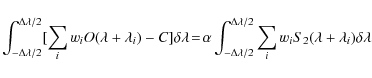
for the 13C14N lines, and an equivalent formula for the 12C15N lines.
The choice of the lines i depends on the quality of the spectra and on particular circumstances, especially the heliocentric distance. Figures 3 and 4 shows that the width of the envelope of the CN band decreases at large r. The relative intensity of the lines of high quantum number drops rapidly. Many lines could be used efficiently for the coadded profiles of comets de Vico or X5 (Fig. A.1), up to 11 for 12C15N and 8 for 13C14N. On the contrary, at large r, a few lines dominate overwhelmingly. As shown in Sect. 7, some blends may become less troublesome far from the nucleus.
![\begin{figure}
\par\includegraphics[angle=-90,width=8.2cm,clip]{11859_11.eps}
\end{figure}](/articles/aa/full_html/2009/32/aa11859-09/img164.png) |
Figure A.1: Coadded observed (solid line) and synthetic (with and without the rare isotopologues) spectra of comet C/2002 X5 (Kudo-Fujikawa). The upper panel is centered on 13C14N lines (in this instance, R1-R6, R14 and R16), the lower one on 12C15N lines (R1-R5, R11-R13, R15-R17). The large number of useable isotopic lines is allowed by the good quality of the spectra used in the combination. Intensity is in arbitrary units. |
| Open with DEXTER | |
R lines of 13C14N and 12C15N with low quantum numbers are slightly blended and also - depending on the spectral resolution - with the corresponding R line of 12C14N. An additional difficulty is the presence of faint lines of the B-X (0-0) band of CH. This region of the spectrum needs special care (e.g., some iterative procedure) and may have to be ignored for the lowest quality spectra.
Appendix B: Averages
While weighted averages of measurements xi with errors ei (
![]() )
are easily defined as
)
are easily defined as
![]() ,
estimating the resulting error on this value is less obvious. The global data set is far from homogeneous. Systematic errors affect the various data sets in different ways. The instrumentation and the circumstances are never identical.
Two estimates of the standard error S are sometimes used:
,
estimating the resulting error on this value is less obvious. The global data set is far from homogeneous. Systematic errors affect the various data sets in different ways. The instrumentation and the circumstances are never identical.
Two estimates of the standard error S are sometimes used:
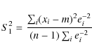
and

They are not satisfying, particularly for a small data set. Equation (B.1) does not take properly into account the individual errors, except for the weighting factors, so that a few xi with large ei but grouped by chance around m would give an unrealistically small S1. On the other hand Eq. (B.2) does not take into account the inter-group variations which can be large in the case of systematic effects. The larger of S1 and S2 may be taken, but we choose a different approach by simulating the xi as the average of ni individual observations yi,j (
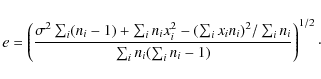
For large
Appendix C: Spectra
![\begin{figure}
\par\includegraphics[angle=270,width=14cm,clip]{11859_12.eps}
\end{figure}](/articles/aa/full_html/2009/32/aa11859-09/img175.png) |
Figure C.1: Observed (2DCoudé) and synthetic (dotted) spectra of comet 122P/de Vico. In this and the following graphs, the upper (red) ticks indicate the position of the major R lines of 13C14N the lower (blue) ticks indicate the position of the major R lines of 12C15N. The corresponding quantum numbers are indicated in the upper panel midway between the strong 12C14N lines and the faint isotopic lines. The intensity scale is in relative units. |
| Open with DEXTER | |
![\begin{figure}
\par\includegraphics[angle=270,width=14cm,clip]{11859_13.eps}
\end{figure}](/articles/aa/full_html/2009/32/aa11859-09/img176.png) |
Figure C.2: Observed (2DCoudé) and synthetic (dotted) spectra of comet C/1996 B2 (Hyakutake). |
| Open with DEXTER | |
![\begin{figure}
\par\includegraphics[angle=270,width=14cm,clip]{11859_14.eps}
\end{figure}](/articles/aa/full_html/2009/32/aa11859-09/img177.png) |
Figure C.3: Observed (2DCoudé) and synthetic (dotted) spectra of comet C/1996 B2 (Hyakutake). |
| Open with DEXTER | |
![\begin{figure}
\par\includegraphics[angle=270,width=14cm,clip]{11859_15.eps}
\end{figure}](/articles/aa/full_html/2009/32/aa11859-09/img178.png) |
Figure C.4: Observed (2DCoudé) and synthetic (dotted) spectra of comet C/1995 O1 (Hale-Bopp). |
| Open with DEXTER | |
![\begin{figure}
\par\includegraphics[angle=270,width=14cm,clip]{11859_16.eps}
\end{figure}](/articles/aa/full_html/2009/32/aa11859-09/img179.png) |
Figure C.5: Observed (2DCoudé) and synthetic (dotted) spectra of comet C/1995 O1 (Hale-Bopp). |
| Open with DEXTER | |
![\begin{figure}
\par\includegraphics[angle=270,width=14cm,clip]{11859_17.eps}
\end{figure}](/articles/aa/full_html/2009/32/aa11859-09/img180.png) |
Figure C.6: Observed (SOFIN) and synthetic (dotted) spectra of comet C/1995 O1 (Hale-Bopp). |
| Open with DEXTER | |
![\begin{figure}
\par\includegraphics[angle=270,width=14cm,clip]{11859_18.eps}
\end{figure}](/articles/aa/full_html/2009/32/aa11859-09/img181.png) |
Figure C.7: Observed (2DCoudé) and synthetic (dotted) spectra of comet 55P/Tempel-Tuttle. |
| Open with DEXTER | |
![\begin{figure}
\par\includegraphics[angle=270,width=14cm,clip]{11859_19.eps}
\end{figure}](/articles/aa/full_html/2009/32/aa11859-09/img182.png) |
Figure C.8: Observed (2DCoudé) and synthetic (dotted) spectra of comet C/1999 H1 (Lee). |
| Open with DEXTER | |
![\begin{figure}
\par\includegraphics[angle=270,width=14cm,clip]{11859_20.eps}
\end{figure}](/articles/aa/full_html/2009/32/aa11859-09/img183.png) |
Figure C.9: Observed (2DCoudé) and synthetic (dotted) spectra of comet C/1999 S4 (LINEAR). |
| Open with DEXTER | |
![\begin{figure}
\par\includegraphics[angle=270,width=14cm,clip]{11859_21.eps}
\end{figure}](/articles/aa/full_html/2009/32/aa11859-09/img184.png) |
Figure C.10: Observed (2DCoudé) and synthetic (dotted) spectra of comet C/1999 T1 (McNaught-Hartley). |
| Open with DEXTER | |
![\begin{figure}
\par\includegraphics[angle=270,width=14cm,clip]{11859_22.eps}
\end{figure}](/articles/aa/full_html/2009/32/aa11859-09/img185.png) |
Figure C.11: Observed (2DCoudé) and synthetic (dotted) spectra of comet C/2001 A2-A (LINEAR). |
| Open with DEXTER | |
![\begin{figure}
\par\includegraphics[angle=270,width=14cm,clip]{11859_23.eps}
\end{figure}](/articles/aa/full_html/2009/32/aa11859-09/img186.png) |
Figure C.12: Observed (UVES) and synthetic (dotted) spectra of comet C/2000 WM1 (LINEAR). |
| Open with DEXTER | |
![\begin{figure}
\par\includegraphics[angle=270,width=14cm,clip]{11859_24.eps}
\end{figure}](/articles/aa/full_html/2009/32/aa11859-09/img187.png) |
Figure C.13: Observed (2DCoudé) and synthetic (dotted) spectra of comet 153P/Ikeya-Zhang. |
| Open with DEXTER | |
![\begin{figure}
\par\includegraphics[angle=270,width=14cm,clip]{11859_25.eps}
\end{figure}](/articles/aa/full_html/2009/32/aa11859-09/img188.png) |
Figure C.14: Observed (UVES) and synthetic (dotted) spectra of comet C/2002 X5 (Kudo-Fujikawa). |
| Open with DEXTER | |
![\begin{figure}
\par\includegraphics[angle=270,width=14cm,clip]{11859_26.eps}
\end{figure}](/articles/aa/full_html/2009/32/aa11859-09/img189.png) |
Figure C.15: Observed (UVES) and synthetic (dotted) spectra of comet C/2002 V1 (NEAT). |
| Open with DEXTER | |
![\begin{figure}
\par\includegraphics[angle=270,width=14cm,clip]{11859_27.eps}
\end{figure}](/articles/aa/full_html/2009/32/aa11859-09/img190.png) |
Figure C.16: Observed (UVES) and synthetic (dotted) spectra of comet C/2002 Y1 (Juels-Holvorcem). |
| Open with DEXTER | |
![\begin{figure}
\par\includegraphics[angle=270,width=14cm,clip]{11859_28.eps}
\end{figure}](/articles/aa/full_html/2009/32/aa11859-09/img191.png) |
Figure C.17: Observed (UVES) and synthetic (dotted) spectra of comet 88P/Howell. |
| Open with DEXTER | |
![\begin{figure}
\par\includegraphics[angle=270,width=14cm,clip]{11859_29.eps}
\end{figure}](/articles/aa/full_html/2009/32/aa11859-09/img192.png) |
Figure C.18: Observed (UVES) and synthetic (dotted) spectra of comet C/2002 T7 (LINEAR). |
| Open with DEXTER | |
![\begin{figure}
\par\includegraphics[angle=270,width=14cm,clip]{11859_30.eps}
\end{figure}](/articles/aa/full_html/2009/32/aa11859-09/img193.png) |
Figure C.19: Observed (UVES) and synthetic (dotted) spectra of comet C/2001 Q4 (NEAT). |
| Open with DEXTER | |
![\begin{figure}
\par\includegraphics[angle=270,width=14cm,clip]{11859_31.eps}
\end{figure}](/articles/aa/full_html/2009/32/aa11859-09/img194.png) |
Figure C.20: Observed (UVES) and synthetic (dotted) spectra of comet C/2001 Q4 (NEAT). |
| Open with DEXTER | |
![\begin{figure}
\par\includegraphics[angle=270,width=14cm,clip]{11859_32.eps}
\end{figure}](/articles/aa/full_html/2009/32/aa11859-09/img195.png) |
Figure C.21: Observed (UVES) and synthetic (dotted) spectra of comet C/2003 K4 (LINEAR). |
| Open with DEXTER | |
![\begin{figure}
\par\includegraphics[angle=270,width=14cm,clip]{11859_33.eps}
\end{figure}](/articles/aa/full_html/2009/32/aa11859-09/img196.png) |
Figure C.22: Observed (UVES) and synthetic (dotted) spectra of comet C/2003 K4 (LINEAR). |
| Open with DEXTER | |
![\begin{figure}
\par\includegraphics[angle=270,width=14cm,clip]{11859_34.eps}
\end{figure}](/articles/aa/full_html/2009/32/aa11859-09/img197.png) |
Figure C.23: Observed (HIRES) and synthetic (dotted) spectra of comet 9P/Tempel 1. |
| Open with DEXTER | |
![\begin{figure}
\par\includegraphics[angle=270,width=14cm,clip]{11859_35.eps}
\end{figure}](/articles/aa/full_html/2009/32/aa11859-09/img198.png) |
Figure C.24: Observed (UVES) and synthetic (dotted) spectra of comet 9P/Tempel 1. |
| Open with DEXTER | |
![\begin{figure}
\par\includegraphics[angle=270,width=14cm,clip]{11859_36.eps}
\end{figure}](/articles/aa/full_html/2009/32/aa11859-09/img199.png) |
Figure C.25: Observed (UVES) and synthetic (dotted) spectra of comet 73P-B/Schwassmann-Wachmann 3. |
| Open with DEXTER | |
![\begin{figure}
\par\includegraphics[angle=270,width=14cm,clip]{11859_37.eps}
\end{figure}](/articles/aa/full_html/2009/32/aa11859-09/img200.png) |
Figure C.26: Observed (2DCoudé) and synthetic (dotted) spectra of comet 73P-B/Schwassmann-Wachmann 3. |
| Open with DEXTER | |
![\begin{figure}
\par\includegraphics[angle=270,width=14cm,clip]{11859_38.eps}
\end{figure}](/articles/aa/full_html/2009/32/aa11859-09/img201.png) |
Figure C.27: Observed (UVES) and synthetic (dotted) spectra of comet 73P-C/Schwassmann-Wachmann 3. |
| Open with DEXTER | |
![\begin{figure}
\par\includegraphics[angle=270,width=14cm,clip]{11859_39.eps}
\end{figure}](/articles/aa/full_html/2009/32/aa11859-09/img202.png) |
Figure C.28: Observed (2DCoudé) and synthetic (dotted) spectra of comet 73P-C/Schwassmann-Wachmann 3. |
| Open with DEXTER | |
![\begin{figure}
\par\includegraphics[angle=270,width=14cm,clip]{11859_40.eps}
\end{figure}](/articles/aa/full_html/2009/32/aa11859-09/img203.png) |
Figure C.29: Observed (2DCoudé) and synthetic (dotted) spectra of comet C/2006 M4 (SWAN). |
| Open with DEXTER | |
![\begin{figure}
\par\includegraphics[angle=270,width=14cm,clip]{11859_41.eps}
\end{figure}](/articles/aa/full_html/2009/32/aa11859-09/img204.png) |
Figure C.30: Observed (HIRES) and synthetic (dotted) spectra of comet 17P/Holmes. |
| Open with DEXTER | |
![\begin{figure}
\par\includegraphics[angle=270,width=14cm,clip]{11859_42.eps}
\end{figure}](/articles/aa/full_html/2009/32/aa11859-09/img205.png) |
Figure C.31: Observed (2DCoudé) and synthetic (dotted) spectra of comet 17P/Holmes. |
| Open with DEXTER | |
![\begin{figure}
\par\includegraphics[angle=270,width=14cm,clip]{11859_43.eps}
\end{figure}](/articles/aa/full_html/2009/32/aa11859-09/img206.png) |
Figure C.32: Observed (2DCoudé) and synthetic (dotted) spectra of comet 8P/Tuttle. |
| Open with DEXTER | |
![\begin{figure}
\par\includegraphics[angle=270,width=14cm,clip]{11859_44.eps}
\end{figure}](/articles/aa/full_html/2009/32/aa11859-09/img207.png) |
Figure C.33: Observed (2DCoudé) and synthetic (dotted) spectra of comet C/2007 N3 (Lulin). |
| Open with DEXTER | |
D Synthetic spectra
![\begin{figure}
\par\includegraphics[width=8.5cm,clip]{11859_45.eps}
\end{figure}](/articles/aa/full_html/2009/32/aa11859-09/img208.png) |
Figure D.1:
Small region of the B-X 0-0 band of the three CN isotopologues.
The synthetic spectra were computed using isotopic abundances of 1, 1/89 and 1/145 for 12C14N (black), 13C14N (red) and 12C15N (blue), respectively, in the absence of collisional effects, and with r=1 AU, |
| Open with DEXTER | |
![\begin{figure}
\par\includegraphics[width=8.5cm,clip]{11859_46.eps}
\end{figure}](/articles/aa/full_html/2009/32/aa11859-09/img209.png) |
Figure D.2: Same as Fig. D.1 for a region of the B-X 0-1 band. |
| Open with DEXTER | |
![\begin{figure}
\par\includegraphics[width=8.5cm,clip]{11859_47.eps}
\end{figure}](/articles/aa/full_html/2009/32/aa11859-09/img210.png) |
Figure D.3: Same as Fig. D.1 for a region of the A-X 2-0 band. |
| Open with DEXTER | |
![\begin{figure}
\includegraphics[width=8.5cm,clip]{11859_48.eps}
\end{figure}](/articles/aa/full_html/2009/32/aa11859-09/img211.png) |
Figure D.4: Same as Fig. D.1 for a region of the A-X 1-0 band. |
| Open with DEXTER | |
Footnotes
- ... comets
- Appendices and Table 8 are only available in electronic form at http://www.aanda.org
- ...
- Based on observations made with ESO Telescopes at the La Silla Paranal Observatory under programmes ID 268.C-5570, 270.C-5043, 073.C-0525, 274.C-5015 and 075.C-0355(A).
- ...
- J.M. is Research Director FNRS, E.J. is Research Associate FNRS and DH is Senior Research Associate FNRS.
- ...
- Deceased on 14 May 2009.
All Tables
Table 1: Relative flux emitted in the various CN bands shown in Fig. 1.
Table 2: Observed comets.
Table 3: Observational circumstances.
Table 4: Isotopic ratios in CN.
Table 5: Lines not identified as CN within the 3857-3880 Å range. Most are not yet identified.
Table 6: Average isotopic ratios. The weighted mean is computed for a variety of groups: all data, all data excluding 73P/Schwassmann-Wachmann 3 B and C, and each of the categories of Levison (JF, HF, EXT, NEW) or Horner et al. (SP, I, L).
Table 7: Isotopic ratios in CN at various nucleocentric distances. The C/2002 T7 (LINEAR) data include spectra taken at up to 180 000 km but are strongly weighted for the range 24 000-45 000 km.
Table 8:
Individual spectra. r is the heliocentric distance in astronomical units (AU), ![]() the geocentric distance, Spectro the spectrograph used,
the geocentric distance, Spectro the spectrograph used,
![]() the Modified Julian Day, Run the run number, Exp the exposure time in seconds, R the spectral resolution. Slit and Offset give the size of the entrance slit of the spectrograph and the offset from the nucleus. T and Q are the parameters used for the collisional effects in the synthetic spectra.
the Modified Julian Day, Run the run number, Exp the exposure time in seconds, R the spectral resolution. Slit and Offset give the size of the entrance slit of the spectrograph and the offset from the nucleus. T and Q are the parameters used for the collisional effects in the synthetic spectra.
All Figures
| |
Figure 1:
Synthetic spectrum of 12C14N over the whole optical domain (r=1 AU, |
| Open with DEXTER | |
| In the text | |
| |
Figure 2:
Variations of of the signal-to-noise ratio
|
| Open with DEXTER | |
| In the text | |
| |
Figure 3:
Synthetic spectra of 12C14N at various heliocentric distances. The intensity scale is arbitrary. The R-branch of the (0-0) band extends shortward of 3875 Å
and the P-branch longward of 3875 Å. Weak lines of the P-branch of the (1-1) band are visible at wavelengths shorter than 3872.5 Å. The black spectra correspond to a collisionless coma with |
| Open with DEXTER | |
| In the text | |
| |
Figure 4: Same as Fig. 3 for 12C15N. |
| Open with DEXTER | |
| In the text | |
| |
Figure 5: Swings effect in the R lines used to estimate the 12C/13C ( top) and 14N/15N ratios. The solid line corresponds to the emission of 12C14N; the red line to the emission of an equal amount of the rare isotopologue; the green line is the ratio 12C/13C or 14N/15N. Intensity is in arbitrary units. Observing comets close to the perihelion is thus particularly interesting because of the weaker contamination by the lines of 12C14N. |
| Open with DEXTER | |
| In the text | |
| |
Figure 6: Variations of the collisional temperature T with the heliocentric distance. |
| Open with DEXTER | |
| In the text | |
| |
Figure 7: 12C/13C and 14N/15N versus the heliocentric distance. The horizontal lines show the mean values (91.0 and 147.8, respectively). Different symbols refer to different comet families. |
| Open with DEXTER | |
| In the text | |
| |
Figure 8: 14N/15N versus 12C/13C. Different symbols refer to different comet families. Small shifts have been introduced to reduce overlapping. |
| Open with DEXTER | |
| In the text | |
| |
Figure 9: Spectra of comet C/2001 Q4 (NEAT) obtained close to the nucleus (solid line) and at about 50 000 km (green dashes). The positions of spatially peaked features appearing only in the nucleus spectrum are shown by dots. CH lines are indicated by + symbols. The upper (red) vertical ticks indicate the position of the main lines of 13C14N the lower (blue) ticks indicate the position of the main lines of 12C15N. The intensity scale is in relative units. |
| Open with DEXTER | |
| In the text | |
| |
Figure A.1: Coadded observed (solid line) and synthetic (with and without the rare isotopologues) spectra of comet C/2002 X5 (Kudo-Fujikawa). The upper panel is centered on 13C14N lines (in this instance, R1-R6, R14 and R16), the lower one on 12C15N lines (R1-R5, R11-R13, R15-R17). The large number of useable isotopic lines is allowed by the good quality of the spectra used in the combination. Intensity is in arbitrary units. |
| Open with DEXTER | |
| In the text | |
| |
Figure C.1: Observed (2DCoudé) and synthetic (dotted) spectra of comet 122P/de Vico. In this and the following graphs, the upper (red) ticks indicate the position of the major R lines of 13C14N the lower (blue) ticks indicate the position of the major R lines of 12C15N. The corresponding quantum numbers are indicated in the upper panel midway between the strong 12C14N lines and the faint isotopic lines. The intensity scale is in relative units. |
| Open with DEXTER | |
| In the text | |
| |
Figure C.2: Observed (2DCoudé) and synthetic (dotted) spectra of comet C/1996 B2 (Hyakutake). |
| Open with DEXTER | |
| In the text | |
| |
Figure C.3: Observed (2DCoudé) and synthetic (dotted) spectra of comet C/1996 B2 (Hyakutake). |
| Open with DEXTER | |
| In the text | |
| |
Figure C.4: Observed (2DCoudé) and synthetic (dotted) spectra of comet C/1995 O1 (Hale-Bopp). |
| Open with DEXTER | |
| In the text | |
| |
Figure C.5: Observed (2DCoudé) and synthetic (dotted) spectra of comet C/1995 O1 (Hale-Bopp). |
| Open with DEXTER | |
| In the text | |
| |
Figure C.6: Observed (SOFIN) and synthetic (dotted) spectra of comet C/1995 O1 (Hale-Bopp). |
| Open with DEXTER | |
| In the text | |
| |
Figure C.7: Observed (2DCoudé) and synthetic (dotted) spectra of comet 55P/Tempel-Tuttle. |
| Open with DEXTER | |
| In the text | |
| |
Figure C.8: Observed (2DCoudé) and synthetic (dotted) spectra of comet C/1999 H1 (Lee). |
| Open with DEXTER | |
| In the text | |
| |
Figure C.9: Observed (2DCoudé) and synthetic (dotted) spectra of comet C/1999 S4 (LINEAR). |
| Open with DEXTER | |
| In the text | |
| |
Figure C.10: Observed (2DCoudé) and synthetic (dotted) spectra of comet C/1999 T1 (McNaught-Hartley). |
| Open with DEXTER | |
| In the text | |
| |
Figure C.11: Observed (2DCoudé) and synthetic (dotted) spectra of comet C/2001 A2-A (LINEAR). |
| Open with DEXTER | |
| In the text | |
| |
Figure C.12: Observed (UVES) and synthetic (dotted) spectra of comet C/2000 WM1 (LINEAR). |
| Open with DEXTER | |
| In the text | |
| |
Figure C.13: Observed (2DCoudé) and synthetic (dotted) spectra of comet 153P/Ikeya-Zhang. |
| Open with DEXTER | |
| In the text | |
| |
Figure C.14: Observed (UVES) and synthetic (dotted) spectra of comet C/2002 X5 (Kudo-Fujikawa). |
| Open with DEXTER | |
| In the text | |
| |
Figure C.15: Observed (UVES) and synthetic (dotted) spectra of comet C/2002 V1 (NEAT). |
| Open with DEXTER | |
| In the text | |
| |
Figure C.16: Observed (UVES) and synthetic (dotted) spectra of comet C/2002 Y1 (Juels-Holvorcem). |
| Open with DEXTER | |
| In the text | |
| |
Figure C.17: Observed (UVES) and synthetic (dotted) spectra of comet 88P/Howell. |
| Open with DEXTER | |
| In the text | |
| |
Figure C.18: Observed (UVES) and synthetic (dotted) spectra of comet C/2002 T7 (LINEAR). |
| Open with DEXTER | |
| In the text | |
| |
Figure C.19: Observed (UVES) and synthetic (dotted) spectra of comet C/2001 Q4 (NEAT). |
| Open with DEXTER | |
| In the text | |
| |
Figure C.20: Observed (UVES) and synthetic (dotted) spectra of comet C/2001 Q4 (NEAT). |
| Open with DEXTER | |
| In the text | |
| |
Figure C.21: Observed (UVES) and synthetic (dotted) spectra of comet C/2003 K4 (LINEAR). |
| Open with DEXTER | |
| In the text | |
| |
Figure C.22: Observed (UVES) and synthetic (dotted) spectra of comet C/2003 K4 (LINEAR). |
| Open with DEXTER | |
| In the text | |
| |
Figure C.23: Observed (HIRES) and synthetic (dotted) spectra of comet 9P/Tempel 1. |
| Open with DEXTER | |
| In the text | |
| |
Figure C.24: Observed (UVES) and synthetic (dotted) spectra of comet 9P/Tempel 1. |
| Open with DEXTER | |
| In the text | |
| |
Figure C.25: Observed (UVES) and synthetic (dotted) spectra of comet 73P-B/Schwassmann-Wachmann 3. |
| Open with DEXTER | |
| In the text | |
| |
Figure C.26: Observed (2DCoudé) and synthetic (dotted) spectra of comet 73P-B/Schwassmann-Wachmann 3. |
| Open with DEXTER | |
| In the text | |
| |
Figure C.27: Observed (UVES) and synthetic (dotted) spectra of comet 73P-C/Schwassmann-Wachmann 3. |
| Open with DEXTER | |
| In the text | |
| |
Figure C.28: Observed (2DCoudé) and synthetic (dotted) spectra of comet 73P-C/Schwassmann-Wachmann 3. |
| Open with DEXTER | |
| In the text | |
| |
Figure C.29: Observed (2DCoudé) and synthetic (dotted) spectra of comet C/2006 M4 (SWAN). |
| Open with DEXTER | |
| In the text | |
| |
Figure C.30: Observed (HIRES) and synthetic (dotted) spectra of comet 17P/Holmes. |
| Open with DEXTER | |
| In the text | |
| |
Figure C.31: Observed (2DCoudé) and synthetic (dotted) spectra of comet 17P/Holmes. |
| Open with DEXTER | |
| In the text | |
| |
Figure C.32: Observed (2DCoudé) and synthetic (dotted) spectra of comet 8P/Tuttle. |
| Open with DEXTER | |
| In the text | |
| |
Figure C.33: Observed (2DCoudé) and synthetic (dotted) spectra of comet C/2007 N3 (Lulin). |
| Open with DEXTER | |
| In the text | |
| |
Figure D.1:
Small region of the B-X 0-0 band of the three CN isotopologues.
The synthetic spectra were computed using isotopic abundances of 1, 1/89 and 1/145 for 12C14N (black), 13C14N (red) and 12C15N (blue), respectively, in the absence of collisional effects, and with r=1 AU, |
| Open with DEXTER | |
| In the text | |
| |
Figure D.2: Same as Fig. D.1 for a region of the B-X 0-1 band. |
| Open with DEXTER | |
| In the text | |
| |
Figure D.3: Same as Fig. D.1 for a region of the A-X 2-0 band. |
| Open with DEXTER | |
| In the text | |
| |
Figure D.4: Same as Fig. D.1 for a region of the A-X 1-0 band. |
| Open with DEXTER | |
| In the text | |
Copyright ESO 2009
Current usage metrics show cumulative count of Article Views (full-text article views including HTML views, PDF and ePub downloads, according to the available data) and Abstracts Views on Vision4Press platform.
Data correspond to usage on the plateform after 2015. The current usage metrics is available 48-96 hours after online publication and is updated daily on week days.
Initial download of the metrics may take a while.