Online Material

Appendix A: Fit to the radially averaged Mercury intensity profiles

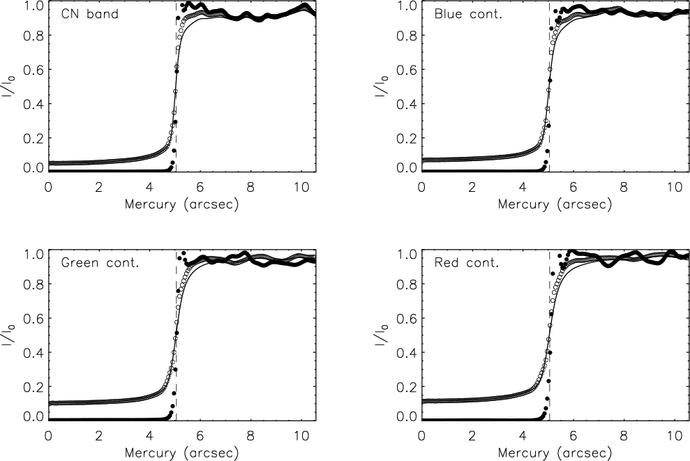$\begin{figure}\par {{\epsfig{file=11975ev1.eps,width=18.0cm} }} \end{figure}$	Figure A.1: The fit to the radially averaged Mercury intensity profiles for CN-band, blue continuum, green continuum, and red continuum wavelengths. Open circles outline the observed intensity profile, the solid line represents the fit to the observed profile and filled circles follow the intensity profile after correction. The vertical dashed line marks the Mercury's limb.
Open with DEXTER

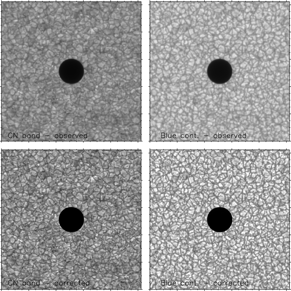$\begin{figure}\par {{\epsfig{file=11975ev2.eps,width=18.0cm} }}\end{figure}$	Figure B.1: Observed ( top) and corrected ( bottom) for CN-band ( left) and blue continuum ( right) wavelengths. Each tick mark corresponds to $\sim$ 2.7 arcsec. The images are cropped to $1024 \times 1024$ pixels, such that Mercury is at the center of the FOV. The original and corrected images at a given wavelength are plotted on the same gray scale.
Open with DEXTER

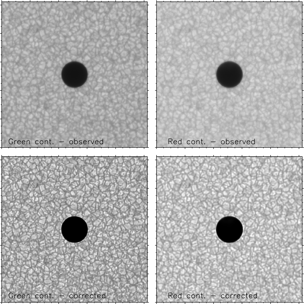$\begin{figure}\par {{\epsfig{file=11975ev3.eps,width=18.0cm} }}\end{figure}$	Figure B.2: Observed ( top) and corrected ( bottom) for green ( left) and red ( right) continuum wavelengths. Each tick mark corresponds to $\sim$ 2.7 arcsec. The images are cropped to $1024 \times 1024$ pixels, such that Mercury is at the center of the FOV. The original and corrected images at a given wavelength are plotted on the same gray scale.
Open with DEXTER