| Issue |
A&A
Volume 501, Number 3, July III 2009
|
|
|---|---|---|
| Page(s) | L19 - L22 | |
| Section | Letters | |
| DOI | https://doi.org/10.1051/0004-6361/200911975 | |
| Published online | 22 June 2009 | |
LETTER TO THE EDITOR
Stray light correction and contrast analysis of Hinode broad-band images![[*]](/icons/foot_motif.png)
S. K. Mathew1,2 - V. Zakharov2 - S. K. Solanki2,3
1 - Udaipur Solar Observatory, PO Box 198, Udaipur 313004, India
2 - Max-Planck-Institut für Sonnensystemforschung (MPS), Max-Planck-Str. 2,
37191 Katlenburg-Lindau, Germany
3 - School of Space Research, Kyung Hee University, Yongin, Gyeonggi 446-701, Korea
Received 2 March 2009 / Accepted 12 June 2009
Abstract
The contrasts of features in the quiet Sun are studied using
filtergrams recorded by the broad-band filter imager mounted on the Hinode/Solar Optical Telescope.
In a first step, the scattered light originating in the instrument is modeled using Mercury transit data. Combinations of four two-dimensional Gaussians with different widths and weights were
employed to retrieve the point-spread functions (PSF) of the instrument at different
wavelengths, which also describe instrumental scattered light.
The parameters of the PSFs at different wavelengths are tabulated. The observed images were then
deconvolved using the PSFs. The corrected images were used to determine the contrasts of features
such as bright points and granulation in different wavelength bands. After correction,
rms contrasts of the granulation of between 0.11 (at 668 nm) and 0.22 (at 388 nm) were obtained.
Similarly, bright point contrasts ranging from 0.07 (at 668 nm) to 0.78 (at 388 nm) are found, which are
a factor of 1.8 to 2.8 higher than those obtained before PSF deconvolution. The mean contrast of the bright
points is found to be somewhat higher in the CN-band than in the G-band, which confirms
theoretical predictions.
Key words: Sun: granulation - Sun: photosphere - instrumentation: high angular resolution
1 Introduction
The contrast of granulation and of magnetic features is an important diagnostic of their thermal structure and provides insight into the energy transport mechanisms acting in them. The contrast of granulation, bright points, and other small scale features is influenced by the point spread function (PSF), the width of whose core is a measure of the spatial resolution, while the strength of the wings is determined by the amount of light scattered within the instrument (or in the atmosphere, if present). In particular, the scattered light strongly reduces the contrast. Bright points, which are smaller in size than the granules, are more strongly affected. If the PSF is known, then it can be used to deconvolve the observed image and thus to recover approximately the original intensities.
Contrasts measured with the Hinode Solar Optical Telescope (SOT, Tsuneta et al. 2008; Suematsu et al. 2008; Kosugi et al. 2007) are of particular interest because of the high spatial resolution and the absence of seeing, leading to almost constant observing conditions. The quality of the Hinode SOT observations would be further enhanced if the PSF could be accurately determined and corrected for (e.g. as achieved by Mathew et al. 2007, for MDI continuum images).
Table 1: Retrieved parameters for four-Gaussian PSFs. Width is specified in arc-secs.
The PSF of the Hinode spectro polarimeter (SP) was determined by Danilovic et al. (2008) by modeling the SOT/SP optical system using the ZEMAX optical design software. After convolving solar granulation data from MHD simulations with the computed PSF, they found that the rms contrast of the simulated granulation closely matches the observations from SOT/SP. Wedemeyer-Böhm (2008) used Mercury transit and eclipse images to determine the PSF of the Hinode/SOT/Broadband Filter Imager (BFI) instrument, but did not apply the obtained PSF to deducing the true contrast in the BFI wavelength bands.
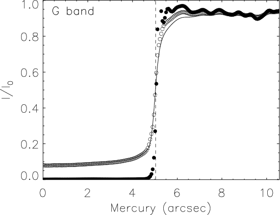 |
Figure 1: The fit to the radially averaged Mercury intensity profile. Open circles outline the observed intensity profile, the solid line represents the fit to the observed profile and filled circles follow the intensity profile after correction. The vertical dashed line marks Mercury's limb. The ripples in the intensity profile outside Mercury's image are mainly due to the average intensity variations in the granules. |
| Open with DEXTER | |
2 Image correction
We used images recorded on 8th Nov. 2006 during a Mercury transit to determine the PSF of the instrument. Full pixel resolution (0.05448 arcsec/pixel) images in the CN and G-bands and also in blue, green, and red continuum bands were available. The theoretical resolution (
In order to derive the PSF of the instrument, we proceeded as follows. The intensity values within
the image of Mercury were replaced by zeros. These images were convolved with a guess PSF,
generated by a combination of four two-dimensional Gaussians. It was found that the use
of four Gaussians, instead of three Gaussians and a Lorentzian as used in Mathew
et al. (2007) for MDI full-disk images, gave a better fit in our case, i.e; for the
Mercury transit images. The Gaussians with appropriate weights and widths are representative of both
the diffraction-limited PSF and the non-ideal part that contributes to the scattered light in the instrument.
By performing a two-dimensional convolution, we ensure that the stray light from all sides
contributes to the intensity within Mercury's image. The sum of the two-dimensional Gaussians
used for the convolution is,
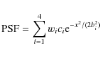
where bi is the width,
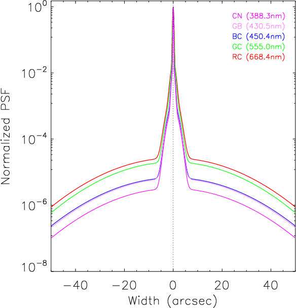 |
Figure 2: PSF for different wavelengths observed by Hinode/SOT/BFI. The corresponding values for the weights and widths of the Gaussian functions are given in Table 1. |
| Open with DEXTER | |
In the next step, the best-fit model parameters were used to retrieve the stray light-free intensities from the observed images. As pointed out by Wedemeyer-Bhöm (2008), the scattering could be anistropic and the resulting PSF could be different for observations from different fields-of-views. Since we assume that the scattering is uniform within the observed field-of-view, we restrict our contrast analysis to about the same part of the image, where the Mercury transit observations were obtained, but avoid the immediate vicinity of Mercury's image to avoid being influenced by artifacts of the deconvolution.
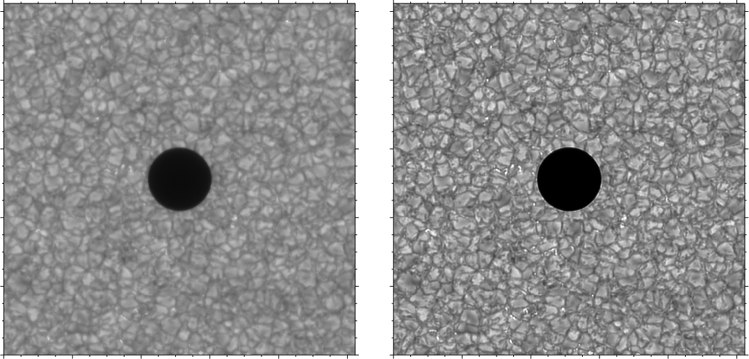 |
Figure 3:
Observed ( left) and corrected ( right) G-band images. Each tick mark corresponds to |
| Open with DEXTER | |
The restoration of the images was carried out using the maximum likelihood deconvolution method (an IDL routine available in Astrolib was used for this purpose; Richarson 1972; Lane 1996). This method invokes an iterative process and updates the current estimate of the image by the product of previous deconvolution results and the correlation between re-convolution of the later image and the PSF. The convergence of restoration is checked from the chi-square of the fit obtained by comparing the observed data and the re-convolved deconvolution results. The filled circles in Fig. 1 show the azimuthally averaged intensity profile across the Mercury image after the deconvolution. The intensity lies close to zero throughout almost the whole of Mercury's image, compared to observed values of 7% or higher in units of averaged quiet-Sun intensity. This indicates that the deconvolution is effective in removing the scattered light. In Fig. 3, an observed G-band image is shown on the left and the corresponding restored image on the right. The higher contrast of the restored image is quite distinctive. Note that both images have been plotted on the same gray-scale (for restored images at other wavelengths, we refer to the additional electronic material to the paper; Figs. B.1 and B.2). A halo-like structure is seen around Mercury in the deconvolved image, which could be caused by Gibb's effect because of the large intensity variation across Mercury's limb. We investigated whether bright points are also affected by comparing the observed and corrected intensity profiles across sample bright points. We did not observed any noticeable signature of Gibb's effect in bright points that could introduce errors in our contrast analysis.
3 Contrast analysis
The deconvolution of the BFI images leads to significant enhancements in the contrast.
This is illustrated by Table 2, which compares the rms contrast of the images
(excluding Mercury and nearby surroundings) and the intensity contrast, C, of
G-band bright
points (BPs) (
C=I/I0-1, where I0 is the average quiet-Sun intensity)
in each filtergram before and after deconvolution. The rms contrast is 1.6 to 2.1 times higher
in deconvolved images than in the originally observed images. Note that since we are dealing with
quiet-Sun data the rms contrast of the image corresponds basically to the granulation contrast,
which lies above 20% at two of the observed wavelengths after correction.
We also compared the retrieved contrasts with the results obtained from
3-D MHD simulations. By a linear fit to the contrasts obtained at different
continuum wavelengths, we inferred an rms contrast of 0.128
(with a 1![]() error of 0.035) at 6302 Å. This value is only 0.017
(i.e. 0.5
error of 0.035) at 6302 Å. This value is only 0.017
(i.e. 0.5![]() )
lower than the
granulation contrast of 0.144 at 6302 Å obtained from 3-D radiation MHD
simulations by Danilovic et al. (2008).
)
lower than the
granulation contrast of 0.144 at 6302 Å obtained from 3-D radiation MHD
simulations by Danilovic et al. (2008).
The BP contrast given in Table 2 also increases after deconvolution of the PSF, by a factor of between 1.8 and 2.8. To identify the BPs, we used a technique described by Berger et al. (1998) with an additional constraint imposed following Langhans et al. (2004). The combination of these methods provided a more reliable BP selection (Zakharov et al. in prep.).
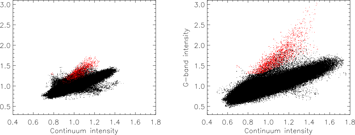 |
Figure 4: Distribution of the G-band intensity versus blue continuum intensity. Red points correspond to BPs, black dots to the remaining features. All intensity values are normalized to the average intensity of that wavelength band. Left frame: before and right frame: after deconvolution of the PSF. |
| Open with DEXTER | |
Table 2: rms contrast of the images and mean BP contrast values obtained before and after deconvolution.
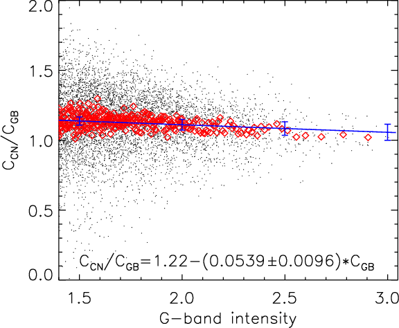 |
Figure 5:
Ratio of BP contrasts in the CN-band and in the G-band versus the
G-band intensity, normalized to its mean. Individual data points are shown as black dots and
red symbols are for the binned data. The solid blue line is a linear regression fit to the
binned data and the error bars for |
| Open with DEXTER | |
The mean BP contrast in the CN-band is higher than in the G-band, both in the original data as
well as in the deconvolved data by a factor of 1.29 and 1.12, respectively.
This finding qualitatively confirms the theoretical predictions
of Berdyugina et al. (2003) and ground-based imaging results (Rutten et al.
2001, Zakharov et al. 2007). Figure 5
displays the dependence of the ratio
![]() on the G-band intensity (after PSF
deconvolution), where
on the G-band intensity (after PSF
deconvolution), where
![]() and
and
![]() are the contrasts of the respective bands as
defined earlier in this section. To obtain the correct slope, we bin together points
with similar G-band intensities such that each bin contains 20 intensity values. The solid line
represents a linear regression fit and the error bars are plotted for
are the contrasts of the respective bands as
defined earlier in this section. To obtain the correct slope, we bin together points
with similar G-band intensities such that each bin contains 20 intensity values. The solid line
represents a linear regression fit and the error bars are plotted for
![]()
![]() deviations
due to the uncertainty in the regression gradient. From this analysis, we obtain a statistically
significant negative slope of 0.054, which indicates that brighter BPs tends to have more similar
CN-band and G-band contrasts. This is in qualitative agreement with the result of Zakharov et al.
(2007).
deviations
due to the uncertainty in the regression gradient. From this analysis, we obtain a statistically
significant negative slope of 0.054, which indicates that brighter BPs tends to have more similar
CN-band and G-band contrasts. This is in qualitative agreement with the result of Zakharov et al.
(2007).
4 Conclusions
Filtergrams recorded by the Hinode/SOT broad-band imager have been used to analyze the contrast of the bright points and the granulation for various wavelength bands. The observed images were deconvolved with the retrieved PSF of the instrument to obtain the original intensities. The retrieved images are nearly free from scattered light and show a 1.6-2.1 times higher rms contrast than the untreated images, while the contrast of BPs increases by a factor of 1.8-2.8. The stronger enhancement of the BP contrast is due to their small size compared to granules, which are mainly responsible for the rms contrast of the whole image.
Acknowledgements
Hinode is a Japanese mission developed and launched by ISAS/JAXA, with NAOJ as domestic partner and NASA and STFC (UK) as international partners. It is operated by these agencies in co-operation with ESA and NSC (Norway). We would like to thank the referee for useful suggestions. This work has been (partially) supported by the WCU grant (No. R31-10016) funded by the Korean Ministry of Education, Science and Technology.
References
- Berdyugina, S. V., Solanki, S. K., & Frutiger, C. 2003, A&A, 412, 513 [NASA ADS] [CrossRef] [EDP Sciences] (In the text)
- Berger, T. E., Löfdahl, M. G., Shine, R. A., & Title, A. M. 1998, ApJ, 506, 439 [NASA ADS] [CrossRef] (In the text)
- Danilovic, S., Gandorfer, A., Lagg, A., et al. 2008, A&A, 484, L17 [NASA ADS] [CrossRef] [EDP Sciences] (In the text)
- Kosugi, T., Matsuzaki, K., Sakao, T., et al. 2008, Sol. Phys., 243, 3 [NASA ADS] [CrossRef] (In the text)
- Lane, R. G. 1996, 2004, J. Opt. Soc. Am., 13, 1992 [CrossRef] (In the text)
- Langhans, K., Schmidt, W., & Rimmele, T. 2004, A&A, 423, L1147 [NASA ADS] [CrossRef] (In the text)
- Mathew, S. K., Martínez Pillet, V., Solanki, S. K., & Krivova, N. A. 2007, A&A, 465, 291 [NASA ADS] [CrossRef] [EDP Sciences] (In the text)
- Richardson, W. H. 1972, J. Opt. Soc. Am., 62, 55 [NASA ADS] [CrossRef] (In the text)
- Rutten, R. J., Kiselman, D., Rouppe van der Voort, L., & Plez, B. 2001, in Advanced solar polarimetry - theory, observation, and instrumentation, ed. M. Sigwarth, ASP Conf. Ser., 236, 445 (In the text)
- Shelyag, S., Schüssler, M., Solanki, S. K., Berdyugina, S. V., & Vögler, A. 2005, A&A, 427, 335 [NASA ADS] [CrossRef] (In the text)
- Suemastu, Y., Tsuneta, S., Ichimoto, K., et al. 2008, Sol. Phys., 249, 197 [NASA ADS] [CrossRef] (In the text)
- Tsuneta, S., Ichimoto, K., Katsukawa, Y., et al. 2008, Sol. Phys., 249, 167 [NASA ADS] [CrossRef] (In the text)
- Wedemeyer-Bhöm, S. 2008, A&A, 487, 399 [NASA ADS] [CrossRef] [EDP Sciences] (In the text)
- Zakharov, V., Gandorfer, A., Solanki, S. K., & Löfdahl, M. 2007, A&A, 461, 695 [NASA ADS] [CrossRef] [EDP Sciences] (In the text)
Online Material
Appendix A: Fit to the radially averaged Mercury intensity profiles
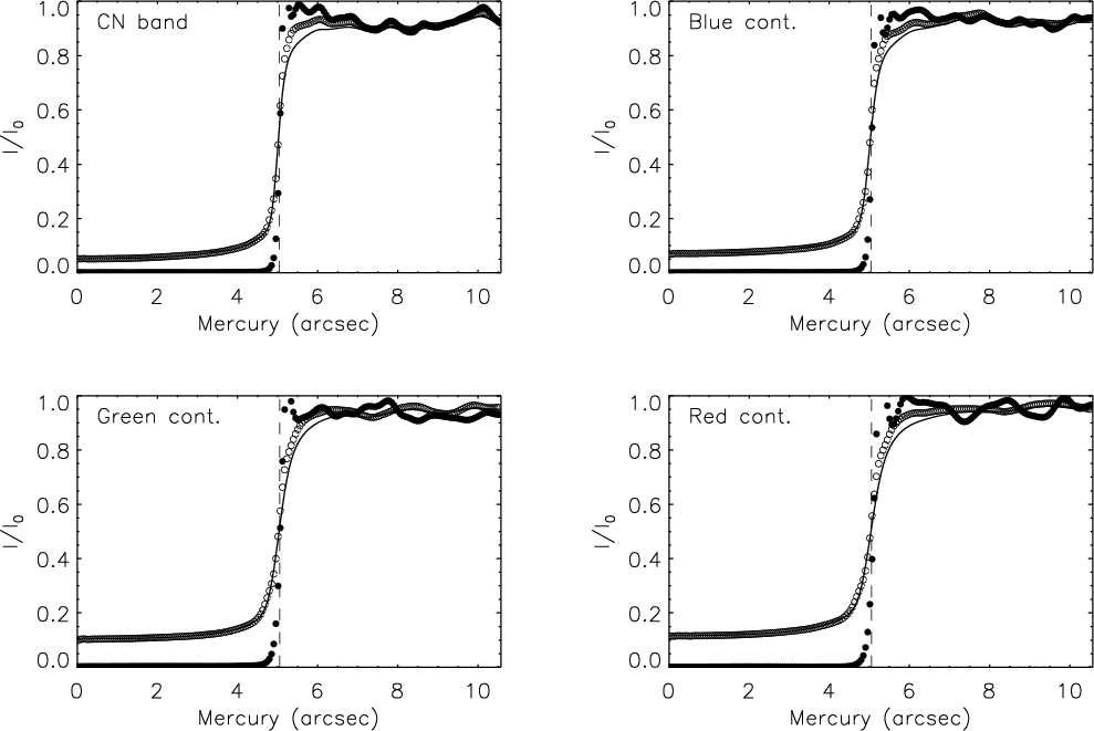 |
Figure A.1: The fit to the radially averaged Mercury intensity profiles for CN-band, blue continuum, green continuum, and red continuum wavelengths. Open circles outline the observed intensity profile, the solid line represents the fit to the observed profile and filled circles follow the intensity profile after correction. The vertical dashed line marks the Mercury's limb. |
| Open with DEXTER | |
Appendix B: Observed and corrected images
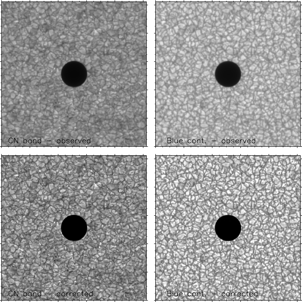 |
Figure B.1:
Observed ( top) and corrected ( bottom) for CN-band ( left) and
blue continuum ( right) wavelengths. Each tick mark corresponds to
|
| Open with DEXTER | |
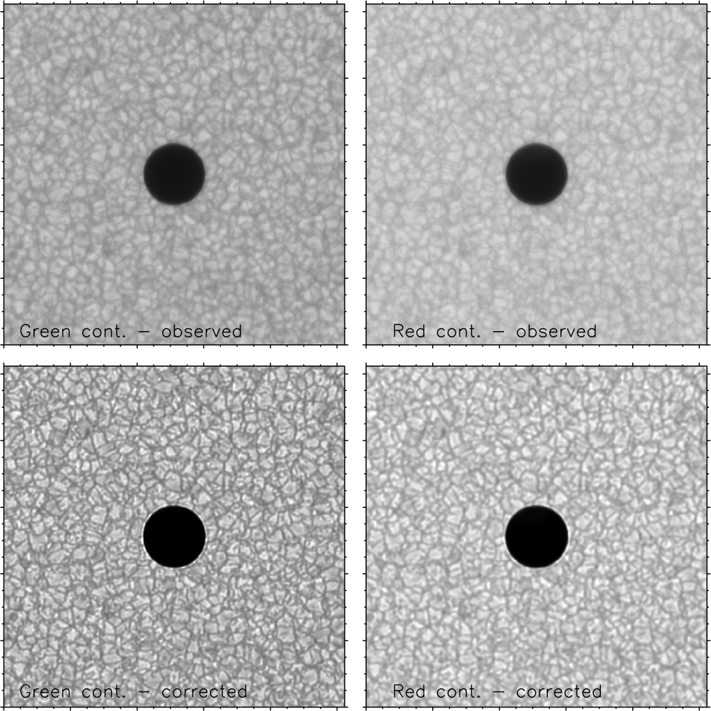 |
Figure B.2:
Observed ( top) and corrected ( bottom) for green ( left)
and red ( right) continuum wavelengths. Each tick mark corresponds to
|
| Open with DEXTER | |
Footnotes
- ... images
- Appendices are only available in electronic form at http://www.aanda.org
All Tables
Table 1: Retrieved parameters for four-Gaussian PSFs. Width is specified in arc-secs.
Table 2: rms contrast of the images and mean BP contrast values obtained before and after deconvolution.
All Figures
| |
Figure 1: The fit to the radially averaged Mercury intensity profile. Open circles outline the observed intensity profile, the solid line represents the fit to the observed profile and filled circles follow the intensity profile after correction. The vertical dashed line marks Mercury's limb. The ripples in the intensity profile outside Mercury's image are mainly due to the average intensity variations in the granules. |
| Open with DEXTER | |
| In the text | |
| |
Figure 2: PSF for different wavelengths observed by Hinode/SOT/BFI. The corresponding values for the weights and widths of the Gaussian functions are given in Table 1. |
| Open with DEXTER | |
| In the text | |
| |
Figure 3:
Observed ( left) and corrected ( right) G-band images. Each tick mark corresponds to |
| Open with DEXTER | |
| In the text | |
| |
Figure 4: Distribution of the G-band intensity versus blue continuum intensity. Red points correspond to BPs, black dots to the remaining features. All intensity values are normalized to the average intensity of that wavelength band. Left frame: before and right frame: after deconvolution of the PSF. |
| Open with DEXTER | |
| In the text | |
| |
Figure 5:
Ratio of BP contrasts in the CN-band and in the G-band versus the
G-band intensity, normalized to its mean. Individual data points are shown as black dots and
red symbols are for the binned data. The solid blue line is a linear regression fit to the
binned data and the error bars for |
| Open with DEXTER | |
| In the text | |
| |
Figure A.1: The fit to the radially averaged Mercury intensity profiles for CN-band, blue continuum, green continuum, and red continuum wavelengths. Open circles outline the observed intensity profile, the solid line represents the fit to the observed profile and filled circles follow the intensity profile after correction. The vertical dashed line marks the Mercury's limb. |
| Open with DEXTER | |
| In the text | |
| |
Figure B.1:
Observed ( top) and corrected ( bottom) for CN-band ( left) and
blue continuum ( right) wavelengths. Each tick mark corresponds to
|
| Open with DEXTER | |
| In the text | |
| |
Figure B.2:
Observed ( top) and corrected ( bottom) for green ( left)
and red ( right) continuum wavelengths. Each tick mark corresponds to
|
| Open with DEXTER | |
| In the text | |
Copyright ESO 2009
Current usage metrics show cumulative count of Article Views (full-text article views including HTML views, PDF and ePub downloads, according to the available data) and Abstracts Views on Vision4Press platform.
Data correspond to usage on the plateform after 2015. The current usage metrics is available 48-96 hours after online publication and is updated daily on week days.
Initial download of the metrics may take a while.