


| Issue |
A&A
Volume 712, August 2026
|
|
|---|---|---|
| Article Number | L3 | |
| Number of page(s) | 5 | |
| Section | Letters to the Editor | |
| DOI | https://doi.org/10.1051/0004-6361/202661336 | |
| Published online | 30 July 2026 | |
Letter to the Editor
Fe Kα line from the broad-line region of PDS456 with XRISM/Resolve
1
INAF – Osservatorio Astronomico di Roma, Via Frascati 33, 00078 Monteporzio, Italy
2
INAF – Istituto di Astrofisica e Planetologia Spaziali, Via del Fosso del Caveliere 100 00133 Roma, Italy
3
Dipartimento di Matematica e Fisica, Universitá degli Studi Roma Tre, Via della Vasca Navale 84 I-00146 Roma, Italy
4
Cahill Center for Astronomy & Astrophysics, California Institute of Technology, 1216 East California Boulevard Pasadena CA 91125, USA
★ Corresponding author: This email address is being protected from spambots. You need JavaScript enabled to view it.
Received:
9
June
2026
Accepted:
11
July
2026
Abstract
The high-luminosity, high-mass and likely super-Eddington quasar PDS 456 is known for its extremely dynamic environment. A wealth of observational features from the millimetric up to the X-ray band shows energetic outflows at all scales, from accretion disc up to galaxy scales. Broad emission lines in the optical and UV show significant widths and line-of-sight velocities. Moreover, NIR interferometry revealed a partially outflowing Broad Line Region. Thanks to the unprecedented energy resolution of the X-ray microcalorimeter Resolve onboard XRISM, we detect a neutral Fe Kα line, the main tracer of cold matter around AGNs. The line blueshift (vout = 2700 km s−1) and width (σ ≤ 700 km s−1) are on the lower bound of the range of values of the optical-UV emission lines, possibly suggesting a stratified medium. The derived column density, NH ≈ 1022 cm−2, is significantly lower than what expected for Broad Line Regions, again in agreement with a composite emission. The very small Equivalent Width (9 eV) marks one of the smallest measurements in the literature and probes the high-luminosity end of the so-called Iwasawa-Taniguchi (or X-ray Baldwin) effect.
Key words: accretion / accretion disks / galaxies: active / quasars: emission lines / quasars: general / quasars: individual: PDS456
© The Authors 2026
 Open Access article, published by EDP Sciences, under the terms of the Creative Commons Attribution License (https://creativecommons.org/licenses/by/4.0), which permits unrestricted use, distribution, and reproduction in any medium, provided the original work is properly cited.
This article is published in open access under the Subscribe to Open model. This email address is being protected from spambots. You need JavaScript enabled to view it. to support open access publication.
1. Introduction
The bright quasar PDS 456 (zPDS = 0.185, Bischetti et al. 2019) stands out as the most luminous active galactic nucleus (AGN) in the nearby (z ≤ 2) Universe, with a bolometric luminosity Lbol ≈ 1047 erg s−1 (Torres et al. 1997; Nardini et al. 2015). Its accretion rate is likely higher than the Eddington rate (GRAVITY Collaboration 2024a; Xrism Collaboration 2025, hereafter X25) and outflowing gas is detected at all spatial scales and wavelengths. Bischetti et al. (2019) detected clumpy outflows in ALMA observations of CO(3-2) line extending at galaxy scales. The gas depletion time is ∼ 8 Myr, indicating that the outflows are able to sweep the galactic gas reservoir, potentially halting the star formation. Likewise, Travascio et al. (2024) detected powerful winds in the optical band with MUSE in [O III] and Hα transitions, extending even beyond the host galaxy.
In the X-ray band, PDS 456 hosts the most clear-cut example of a Fe XXV-XXVI P-Cygni profile due to a massive, highly ionised wind originating at accretion disc scales (Nardini et al. 2015; Luminari et al. 2018). Such powerful outflow has been recently detected at high resolution with the microcalorimeter Resolve (Tashiro et al. 2020) on board XRISM (X25). The huge improvement with respect to previous, CCD-based observations finally resolved the broad absorption through in a number of narrow layers with line-of-sight (LOS) velocities vout = 0.22 − 0.33 c, each one with column density NH ≈ 1023 cm−2 and line broadening σturb ≈ 2000 km s−1. The global mass outflow rate is of the order of 100 M⊙ yr−1, resulting in a kinetic power Ėkin ≈ 1047 erg s−1, of the same order of Lbol (Nardini et al. 2015). Such huge energy output is well above the Ėkin ≥ 0.5% − 5% Lbol theoretical threshold for the outflows to efficiently impact the host galaxy (Hopkins & Elvis 2010; Faucher-Giguère & Quataert 2012; King & Pounds 2015). However, the galactic-scale outflow counterparts detected at optical to millimetric wavelengths are way less energetic than expected, being more consistent with a momentum-conserving propagation rather than with an energy-conserving one, possibly signalling different propagation scenarios at such high luminosity regimes (see Bischetti et al. 2019; Travascio et al. 2024 for further details). Outflows have also been detected with the JWST (Seebeck et al. 2024), mainly from dust and molecular lines, as well as Paα, [O III], [Ne III] and [Ne VI].
Broad emission lines (BELs) in PDS 456 show blueshifted profiles with a quite high broadening, with a full width at half maximum (FWHM) ranging between 3500 km s−1 for the Hhdrogen Balmer series (Simpson et al. 1999) and 15000 km s−1 for C IV (O’Brien et al. 2005). Near-infrared (NIR) interferometry carried out with VLT/GRAVITY spatially resolved the Paα line from the broad-line region (BLR), finding evidence for a partially bound gas, with LOS outflow velocities up to 2000 km s−1. Therefore, all the spectral features, from the NIR up to the UV, lead to the picture of an outflowing BLR. While this is not at all unprecedented (see discussion in GRAVITY Collaboration 2024a, and references therein), such extreme velocities may suggest that PDS 456 is probing the BLR behaviour at extreme quasar luminosities.
In this Letter we report the first detection of a blueshifted fluorescent Fe Kα line in PDS 456, observed in the Resolve spectrum first reported in X25. This adds a further intriguing piece in the puzzle of the dynamic structure of this quasar and represents a valuable probe of the dense matter at the high-luminosity end of the AGN population.
2. Data reduction
XRISM observed PDS 456 during the Performance Verification Phase, from 11 to 17 March 2024. Data were retrieved from the mission archive1 and processed with the latest available pipeline, provided within the Heasoft v6.362, and calibration database (CALDB Resolve files v.20250915). The Resolve data and the non-X-Ray Background (NXB) were reduced following standard prescriptions3 and excluding the calibration pixel, no. 12, and pixel no. 27 due to known gain calibration issues. We extracted the spectrum with different thresholds for the geomagnetic cut-off rigidity (COR). Setting COR > 8, the most conservative choice, results in 187 ksec net exposure time, while COR > 4 yields 260 ksec. Since the two datasets are fully consistent with each other, we use the latter from now on (see Appendix A for more details).
In this Letter we focus on the Fe Kα feature. Therefore, we do not report on the complementary XRISM/Xtend, XMM-Newton and NuSTAR data, since their CCD energy resolutions of hundreds of eV do not allow for a meaningful detection of this feature which, as is shown in the following, has an equivalent width (EW) of the order of 9 eV. In the following we use the xspec fitting package (Arnaud 1996). Unless when stated otherwise, we binned the data to 5 eV resolution, the nominal energy resolution of Resolve, and we emploied the Cash statistics (Cash 1976). However, consistent results were obtained binning to lower (2 eV) or higher (10 or 15 eV) energy intervals.
3. Spectral analysis
3.1. Broadband inspection
The X-ray spectrum of PDS 456 is notoriously complex. The intrinsic continuum is well described by a powerlaw with photon index Γ = 2.0 − 2.3 and no evidence for reflection (Nardini et al. 2015, X25). This continuum is reprocessed by the many intervening winds, both in the soft and in the hard X-ray bands. The massive, highly ionised and mildly relativistic disc winds are responsible for the bright Fe K emission, mostly due to H- and He-like ions (Luminari et al. 2018). Due to the high outflow velocities (between 0.2 and 0.3 c, see above), the emission profile is relativistically broadened and extends from 6 to 8 keV. Bluewards of that, the high-resolution Resolve spectrum shows several highly blueshifted Fe K absorption lines strongly affecting the underlying continuum up to around 10 keV, after which the spectrum becomes background-dominated (see Fig. 3 of X25). In order to visually inspect the spectrum, we first fit the whole 2 − 10 keV energy band with the following phenomenological model:
 (1)
(1)
The model consists of a power-law continuum and a broad Gaussian emission line to account for the wind emission. The source spectrum is absorbed by a TBabs (Wilms et al. 2000) cold absorption component with a Galactic column of NH = 2 × 1021 cm−2 (as per HI4PI Collaboration 2016). Hereafter, the NXB spectrum is always included and fitted jointly with the source spectrum using the empirical model made available by the Science Team4, which is composed by a flat power law (Γ = 0.14) with several narrow neutral emission lines. The best-fit result is shown in Fig. A.1. The power-law component has Γ = 2.07 ± 0.08 and normalisation (1.6 ± 0.2) × 10−3 ph cm−2 s−1 keV−1 at 1 keV. Gausswind has line energy = 4.9 ± 0.2 keV, a broadening σ = 1.5 ± 0.2 keV, and EW = 3.4 ± 0.7 keV. The 2-10 keV flux is 5.6⋅10−12 erg s−1 cm−2, corresponding to 5.5⋅1044 erg s−1.
By inspecting the residuals, we note an excess emission at E ≈ 5.45 keV (see Fig. 1, middle panel), corresponding to 6.46 keV source-frame, slightly blueshifted with respect to the energy of the Fe Kα line. Therefore, we focus on a narrow spectral interval to accurately characterise this excess.
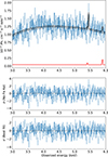 |
Fig. 1. Spectral fit of the 3 − 6 keV band. Top: Data and best-fit model. The red line shows the NXB model, the dashed black line the source model and the solid black line the composition of the two. Centre and bottom panels: Residuals (in units of σ) without and with the Fe Kα line. Spectrum has been re-binned to 15 eV for plotting purposes only. |
3.2. Narrow-band fit
In the following, we restrict the analysis to the 3 − 6 keV energy range. Such interval is sufficiently narrow that the continuum can be reliably described with the simple model in Eq. (1) and yet wide enough to allow for it to be solidly determined (see Shu et al. 2010 for the same approach with high-resolution Chandra grating spectra). This approach is only to present a good analytical description of the continuum and to characterise the narrow line on top of it. We do not attempt to draw any physical conclusions associated with the continuum properties from this analysis.
To model the Fe Kα line we add a zbfeklor component, a composition of seven Lorentzians obtained as the empirical fit to high-resolution laboratory measurements of the fluoresecent neutral Fe Kα line (Hölzer et al. 1997). Such a component represents the standard in high-resolution spectroscopy and it is widely employed for high signal-to-noise Resolve data (see e.g. Yamada et al. 2025; Xrism Collaboration 2026; Bianchi et al. 2026). The only free parameters are the normalisation, the overall velocity broadening σ and the blue/red-shift z of the line energy with respect to the laboratory value. We fit leaving all the parameters free to vary, obtaining a fit statistics of 601.6 for 592 degrees of freedom. Note that replacing zbfeklor with a Gaussian component would lead to fully consistent results but with a ΔC-stat increase of 2.
Figure 1 shows the best fit and the residuals, both without and with the Fe Kα line. The source model is plotted with a dashed black line, while the solid black line shows the total model including the NXB (in red). The nearest NXB line has an energy of 5.415 keV, around eight resolution elements from the peak of the observed line (5.452 keV) and a factor ≈20 lower strength, and therefore it is quite negligible. Table 1 reports the best-fit values with the associated 1σ uncertainties. The statistical improvement upon the inclusion of the Fe Kα is ΔCstat = 11.23. The line EW in the source-frame is  eV, obtained by dividing the observed one by (1+zPDS). Thanks to the unprecedented energy resolution of Resolve, the upper limit of the line broadening is σ ≤ 310(694) km s−1 at 1σ (90 %) c.l., corresponding to an energy width ≤5.6 (12.6) eV. Surprisingly, the redshift is smaller than the systemic one of PDS 456 (zPDS = 0.185), implying vout = 2700 ± 300 km s−1 (90% c.l.). To provide a more physical picture, Fig. 2 shows the contour plot (with 1, 2, 3σ confidence levels) between the derived Fe Kα1 line energy (in the PDS 456 source frame), and the total feature EW. Note that we are ascribing the feature to neutral iron (Fe II). As discussed in Palmeri et al. (2003), Bianchi et al. (2026), mildly ionised Fe would have lower line energies, resulting in higher vout, at least up to Fe X. At higher ionisation states, instead, the Fe line energies increase. However, a certain amount of ionisation is required to have non-negligible fractions of non-neutral iron. This would lead to a distribution of ionic abundances and, then, to several emission lines with comparable strength, which are not detected in the present observation. Therefore, our assumption is the most conservative.
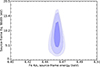 |
Fig. 2. Contour plot between the derived Fe Kα1 line energy (x-axis) and the overall line Equivalent Width (y-axis), both in the PDS 456 source frame. Confidence levels correspond to 1,2,3σ for two parameters of interest. |
Best-fit values of the 3–6 keV fit of the COR> 4 spectrum.
To assess the significance of the Fe Kα line we simulate 104 XRISM/Resolve spectra using the best-fit model removing the line as input, with the same exposure and luminosity as the observation. After fitting the continuum, we search for (spurious) emission features first by fixing the line energy to the observed one and leaving the normalisation and broadening free to vary and, then, leaving also the energy free within a range encompassing the BEL velocities, 0 ≤ vout ≤ 104 km s−1 (see below), i.e. between 5.40 and 5.59 keV. In the first case, we detect a line with a ΔCstat improvement higher than our observed line (=11.23) in 4 spectra, implying a statistical significance > 99.9% (corresponding to > 3σ), while in the second case in 108 spectra, corresponding to > 98.9%.
4. Discussion and conclusions
4.1. The Fe Kα line and the broad emission lines
The BELs of PDS 456 are known for their extreme velocity and broadening. In the UV, a broad and blueshifted C IV emission line has been detected in a Hubble Space Telescope/STIS observation by O’Brien et al. (2005) with vout = 5240 km s−1, FWHM ≈ 15 000 km s−1. They also detected unresolved Si IV/O IVλ1400 lines with vout = 4000 km s−1, FWHM ≈ 7000 km s−1 and Lyα/N Vλ1240 with vout = 600 − 2000 km s−1 and FWHM ≈ 12000 km s−1. In the same spectrum, Hamann et al. (2018) claim the presence of a C IV broad absorption line with vout = 0.3c, FWHM = 8550 km s−1, possibly representing a lower-ionisation phase of the powerful X-ray winds. In the optical band, Simpson et al. (1999) report a He I line with FWHM ≈ 7000 km s−1 and Hα, Hβ and Hγ lines with FWHM ≈ 3500 km s−1 from a spatially unresolved observation. Similarly, the nuclear region of the MUSE IFU observation in Travascio et al. (2024) shows a Hα line with FWHM ≈ 2500 km s−1 and vout ≈ 350 km s−1. Finally, high-resolution NIR interferometry with GRAVITY resolved the BLR through the Paα line (GRAVITY Collaboration 2017, 2024a,b). They modelled the BLR as an ensemble of non-interacting ‘cloudlets’ in rough axisymmetric configuration around the central black hole. Such a model best-fitted the data through a combination of rotational and outflowing motion. The BLR is located at r = 1.33 pc, with an inclination i = 13° (almost face-on) with respect to the LOS. Around 50% of the cloudlets have non-bound orbits, reaching LOS velocities vout ≈ 2000 km s−1. The total line FWHM is of the same order.
The upper limit for the Fe Kα FWHM, 1634 (3758) km s−1 at 1σ (90%) c.l. is at the low end of the above range of values. This may point to a stratified BLR, with closer, broader UV BELs, intermediate optical lines and Fe Kα as the outer layer. The Fe Kα FWHM can be converted into a rotational radius  , where we adopt the same black hole mass MBH = 1.7 × 10⁸ M⊙ and inclination i = 13o (i.e. almost face-on) of GRAVITY for consistency (GRAVITY Collaboration 2024b)5. This value is remarkably similar to the radial location of the X-ray disc wind, between 0.005 and 0.015 pc, estimated in X25, and may indicate that such wind is co-spatial with the BELs, possibly representing a different component that is not gravitationally bound. To get an estimate on the accretion disc size, we compute the dust sublimation radius rsub as the inner boundary of the surrounding cold ‘torus’. It can be computed as
  , where Lbol/1045 erg s−1 and Asub = 0.4 for a sublimation temperature of 1500 K (Barvainis 1987; Nenkova et al. 2008).
4.2. Probing the torus and the X-Ray Baldwin effect at the high-luminosity end
The strength, energy and profile of the Fe Kα line is a powerful probe of the covering factor and the column density of the cold reflector. In the Thomson-thin regime, the line flux IFeKα can be related to these quantities as in Eq. (3) of Yaqoob et al. (2001):
 (2)
(2)
where IFe Kα is in ph cm−2 s−1 (=1.2 ⋅ 10−6, see above), 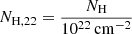 , the powerlaw normalisation Npl is in 10−3 ph keV−1 cm−2 s−1 at 1 keV, fcov = ΔΩ/4π is the fraction of the solid angle covered by the reflector. We set Γ = 2.3, Npl, −3 = 3.4 from the detailed, self-consistent broadband fit of X25. We correct for the updated cross-sections as in Murphy & Yaqoob (2009). Therefore, NH must be of the order of 1022 cm−2 for plausible values of fcov; using the GRAVITY best-fit as an example (fcov = 0.67) we get NH = 5.5 × 1022 cm−2. These values are somewhat lower than the ‘typical’ values for BLR ≈ 1023 cm−2 (see e.g. Osterbrock & Ferland 2006; Netzer 2013), in agreement with the Fe Kα line tracing the outer layer of a stratified BLR.
In the broad AGN population, the EW of the neutral Fe Kα line is found to be anti-correlated with the X-ray continuum luminosity, an effect generally known as the Iwasawa-Taniguchi (or X-Ray Baldwin) effect (e.g. Iwasawa & Taniguchi 1993; Bianchi et al. 2007; Shu et al. 2010, 2012). Although the physical driver is still debated, such effect testifies the evolution of the reflecting matter as a function of the AGN luminosity. Our derived EW = 9 eV is significantly smaller than the expected value of 41±5 eV obtained through the relation in Bianchi et al. (2007) (see also Shu et al. 2010, 2012 for consistent results) for the luminosity of the present observation, L2−10 keV = 4.7 × 1044 erg s−1. PDS 456 is known to exhibit dramatic spectral and flux variations on timescales as short as 30 ksec (Reeves et al. 2002). Albeit quite variable, with a historical average L2−10 keV ≈ 1045 erg s−1 (Nardini et al. 2015), the source sits at the high-luminosity end of the distribution in Bianchi et al. (2007)6. Therefore, it is possible that the observed EW may signal a deviation from the established relation at the highest luminosities. We also note that our value is among the lowest measured EWs in the literature, thanks to the unprecedented resolving power of Resolve in the hard X-ray band.
Acknowledgments
AL, FN acknowledge financial support from grants: EU HORIZON-2020 grant “AHEAD2020” (Agreement No. 871158), ASI Contract No. 2019-27-HH.0 on Athena, PRIN MUR 2022 (DRAGON; No. 2022K9N5B4) and INAF-AF-2023 “The XRISM-to-XIFU (X2X)”, ob.f. 1.05.23.01.06.
References
- Arnaud, K. A. 1996, in ASP Conf. Ser. 101: Astronomical Data Analysis Software and Systems V, 17 [Google Scholar]
- Barvainis, R. 1987, ApJ, 320, 537 [Google Scholar]
- Bianchi, S., Guainazzi, M., Matt, G., & Fonseca Bonilla, N. 2007, A&A, 467, L19 [NASA ADS] [CrossRef] [EDP Sciences] [Google Scholar]
- Bianchi, S., Vander Meulen, B., Bertola, E., et al. 2026, A&A, 710, A274 [NASA ADS] [CrossRef] [EDP Sciences] [Google Scholar]
- Bischetti, M., Piconcelli, E., Feruglio, C., et al. 2019, A&A, 628, A118 [NASA ADS] [CrossRef] [EDP Sciences] [Google Scholar]
- Cash, W. 1976, A&A, 52, 307 [NASA ADS] [Google Scholar]
- Faucher-Giguère, C.-A., & Quataert, E. 2012, MNRAS, 425, 605 [Google Scholar]
- GRAVITY Collaboration (Abuter, R., et al.) 2017, A&A, 602, A94 [NASA ADS] [CrossRef] [EDP Sciences] [Google Scholar]
- GRAVITY Collaboration (Amorim, A., et al.) 2024a, A&A, 690, A76 [Google Scholar]
- GRAVITY Collaboration (Amorim, A., et al.) 2024b, A&A, 684, A167 [NASA ADS] [CrossRef] [EDP Sciences] [Google Scholar]
- Hamann, F., Chartas, G., Reeves, J., & Nardini, E. 2018, MNRAS, 476, 943 [NASA ADS] [CrossRef] [Google Scholar]
- HI4PI Collaboration (Ben Bekhti, N., et al.) 2016, A&A, 594, A116 [NASA ADS] [CrossRef] [EDP Sciences] [Google Scholar]
- Hölzer, G., Fritsch, M., Deutsch, M., Härtwig, J., & Förster, E. 1997, Phys. Rev. A, 56, 4554 [CrossRef] [Google Scholar]
- Hopkins, P. F., & Elvis, M. 2010, MNRAS, 401, 7 [NASA ADS] [CrossRef] [Google Scholar]
- Iwasawa, K., & Taniguchi, Y. 1993, ApJ, 413, L15 [NASA ADS] [CrossRef] [Google Scholar]
- King, A., & Pounds, K. 2015, ARA&A, 53, 115 [NASA ADS] [CrossRef] [Google Scholar]
- Luminari, A., Piconcelli, E., Tombesi, F., et al. 2018, A&A, 619, A149 [NASA ADS] [CrossRef] [EDP Sciences] [Google Scholar]
- Murphy, K. D., & Yaqoob, T. 2009, MNRAS, 397, 1549 [Google Scholar]
- Nardini, E., Reeves, J. N., Gofford, J., et al. 2015, Science, 347, 860 [Google Scholar]
- Nenkova, M., Sirocky, M. M., Nikutta, R., Ivezić, Ž., & Elitzur, M. 2008, ApJ, 685, 160 [Google Scholar]
- Netzer, H. 2013, The Physics and Evolution of Active Galactic Nuclei (Cambridge, UK: Cambridge University Press) [Google Scholar]
- O’Brien, P. T., Reeves, J. N., Simpson, C., & Ward, M. J. 2005, MNRAS, 360, L25 [CrossRef] [Google Scholar]
- Osterbrock, D., & Ferland, G. J. 2006, in Astrophysics of Gaseous Nebulae and Active Galactic Nuclei, eds. D. E. Osterbrock, & G. J. Ferland [Google Scholar]
- Palmeri, P., Mendoza, C., Kallman, T. R., Bautista, M. A., & Meléndez, M. 2003, A&A, 410, 359 [NASA ADS] [CrossRef] [EDP Sciences] [Google Scholar]
- Reeves, J. N., Wynn, G., O’Brien, P. T., & Pounds, K. A. 2002, MNRAS, 336, L56 [NASA ADS] [CrossRef] [Google Scholar]
- Seebeck, J., Veilleux, S., Liu, W., et al. 2024, ApJ, 976, 240 [Google Scholar]
- Shu, X. W., Yaqoob, T., & Wang, J. X. 2010, ApJS, 187, 581 [NASA ADS] [CrossRef] [Google Scholar]
- Shu, X. W., Wang, J. X., Yaqoob, T., Jiang, P., & Zhou, Y. Y. 2012, ApJ, 744, L21 [NASA ADS] [CrossRef] [Google Scholar]
- Simpson, C., Ward, M., O’Brien, P., & Reeves, J. 1999, MNRAS, 303, L23 [NASA ADS] [CrossRef] [Google Scholar]
- Tashiro, M., Maejima, H., Toda, K., et al. 2020, in Space Telescopes and Instrumentation 2020: Ultraviolet to Gamma Ray, eds. J. W. A. den Herder, S. Nikzad, & K. Nakazawa, SPIE Conf. Ser., 11444, 1144422 [NASA ADS] [Google Scholar]
- Torres, C. A. O., Quast, G. R., Coziol, R., et al. 1997, ApJ, 488, L19 [NASA ADS] [CrossRef] [Google Scholar]
- Travascio, A., Piconcelli, E., Bischetti, M., et al. 2024, A&A, 686, A250 [NASA ADS] [CrossRef] [EDP Sciences] [Google Scholar]
- Wilms, J., Allen, A., & McCray, R. 2000, ApJ, 542, 914 [Google Scholar]
- Xrism Collaboration (Audard, M., et al.) 2025, Nature, 641, 1132 [Google Scholar]
- Xrism Collaboration (Audard, M., et al.) 2026, ApJ, 1003, 156 [Google Scholar]
- Yamada, S., Hell, N., Costantini, E., et al. 2025, PASJ, 77, 1210 [Google Scholar]
- Yaqoob, T., George, I. M., Nandra, K., et al. 2001, ApJ, 546, 759 [Google Scholar]
We note that Nardini et al. (2015) report a quite different MBH = 1.2 × 10⁹ M⊙, based on single-epoch BLR scaling relations. Adopting such value would imply a larger rotational radius.
Formally, luminosities in the Shu et al. (2010, 2012) sample reach 1047 erg s−1. However, they are computed by rigidly extrapolating a simple, local power law fit in the 2 − 7 keV band and are therefore less accurate than the self-consistent analysis in Bianchi et al. (2007).
Appendix A: Comparison between COR> 4 and > 8 datasets
Fig. A.1 compares the spectra for COR> 4 and > 8. Top and middle panels report the data and the best fits for the model in Eq. 1 and the associated residuals. See Sect. 3 for details. All best-fit values are fully consistent in the two cases. Bottom panel shows the “difference spectrum”, computed as the difference between the two spectra, with errors in units of σ. Such spectrum is consistent with zero, showing that there are no significant differences between the two datasets. The spectra have been binned to 15 eV for visual clarity.
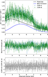 |
Fig. A.1. XRISM/Resolve spectra and best-fit models (top) and residuals (middle) of PDS 456 with cutoff rigidity COR> 4 and COR> 8 (blue and green points, respectively). The best-fit model components are plotted both together and separately, as detailed in the legend. Bottom panels shows the “difference spectrum” between the two datasets. The non X-ray background is not shown here for the sake of clarity. |
All Tables
All Figures
|
Fig. 1. Spectral fit of the 3 − 6 keV band. Top: Data and best-fit model. The red line shows the NXB model, the dashed black line the source model and the solid black line the composition of the two. Centre and bottom panels: Residuals (in units of σ) without and with the Fe Kα line. Spectrum has been re-binned to 15 eV for plotting purposes only. |
| In the text | |
|
Fig. 2. Contour plot between the derived Fe Kα1 line energy (x-axis) and the overall line Equivalent Width (y-axis), both in the PDS 456 source frame. Confidence levels correspond to 1,2,3σ for two parameters of interest. |
| In the text | |
|
Fig. A.1. XRISM/Resolve spectra and best-fit models (top) and residuals (middle) of PDS 456 with cutoff rigidity COR> 4 and COR> 8 (blue and green points, respectively). The best-fit model components are plotted both together and separately, as detailed in the legend. Bottom panels shows the “difference spectrum” between the two datasets. The non X-ray background is not shown here for the sake of clarity. |
| In the text | |
Current usage metrics show cumulative count of Article Views (full-text article views including HTML views, PDF and ePub downloads, according to the available data) and Abstracts Views on Vision4Press platform.
Data correspond to usage on the plateform after 2015. The current usage metrics is available 48-96 hours after online publication and is updated daily on week days.
Initial download of the metrics may take a while.