


| Issue |
A&A
Volume 712, August 2026
|
|
|---|---|---|
| Article Number | A4 | |
| Number of page(s) | 11 | |
| Section | Astrophysical processes | |
| DOI | https://doi.org/10.1051/0004-6361/202659779 | |
| Published online | 30 July 2026 | |
Λ effect in rotating hydrodynamic convection
Institute for Solar Physics (KIS), Georges-Köhler-Alle 401a, 79110 Freiburg im Breisgau, Germany
★ Corresponding author: This email address is being protected from spambots. You need JavaScript enabled to view it.
Received:
10
March
2026
Accepted:
7
May
2026
Abstract
Context. Rotating anisotropic convection generates differential rotation in stellar convection zones.
Aims. The main aim is to compute the non-diffusive contribution (Λ effect) to angular momentum transport – described by Reynolds stress – from rotating turbulent convection.
Methods. Rotating hydrodynamic convection is simulated in Cartesian geometry at different latitudes and rotation rates. Large-scale flows are suppressed such that the Reynolds stress is due to non-diffusive effects.
Results. The radial angular momentum flux is downward (outward) for slow (fast) rotation. This is in contrast with prevailing theories in mean-field hydrodynamics, where the radial transport is always downward. The outward transport at rapid rotation is due to thermal Rossby waves that manifest as elongated large-scale convection cells near the equator. The horizontal angular momentum flux is always equatorward, with increasing concentration towards the equator as in earlier Cartesian studies. The magnitudes of the Λ effect coefficients are roughly an order of magnitude lower than in the case of anisotropically forced turbulence or in analytic theories.
Conclusions. The current results highlight the tension between numerical simulations, widely used mean-field models, and solar observations. The mean-fields models have been remarkably successful in reproducing solar differential rotation but underlying assumptions regarding turbulence in these models seem to be at odds with 3D simulations. The current simulation results for the vertical (radial) angular momentum transport are in accordance with spherical shell simulations, where thermal Rossby waves are responsible for the generation of equatorial acceleration or solar-like differential rotation. Thermal Rossby waves are typically absent in the turbulence models of current mean-field theories, and they have not been unambiguously detected in the Sun.
Key words: convection / turbulence
© The Authors 2026
 Open Access article, published by EDP Sciences, under the terms of the Creative Commons Attribution License (https://creativecommons.org/licenses/by/4.0), which permits unrestricted use, distribution, and reproduction in any medium, provided the original work is properly cited.
This article is published in open access under the Subscribe to Open model. This email address is being protected from spambots. You need JavaScript enabled to view it. to support open access publication.
1. Introduction
Observations of the Sun and other stars with convective envelopes show that differential rotation is ubiquitous (e.g. Rüdiger et al. 2013; Reinhold & Gizon 2015). The main driver of differential rotation has long been thought to be non-vanishing Reynolds stress due to the interaction of rotation and convective turbulence (e.g. Rüdiger 1989):
 (1)
(1)
where  is the fluctuating velocity and where the overbar denotes a suitably defined average. More specifically, the off-diagonal components of Qij have non-diffusive contributions in anisotropic turbulence that are proportional to the angular velocity, Ω, which lead to the generation of differential rotation. This is more commonly known as the Λ effect (e.g. Rüdiger 1980).
The Λ effect has been studied with simulations of anisotropically forced turbulence (Käpylä & Brandenburg 2008; Käpylä 2019b,a; Barekat et al. 2021). These results have confirmed the existence of the Λ effect and are in broad agreement with mean-field hydrodynamics (Rüdiger 1989). Convection simulations show qualitatively similar results at slow rotation (e.g. Pulkkinen et al. 1993; Rüdiger et al. 2005, 2019; Hupfer et al. 2005; Rüdiger & Küker 2021), but differences arise at rapid rotation where, for example, the radial angular momentum flux changes sign (Chan 2001; Käpylä et al. 2004). The latter arises due to large-scale wave-like convective modes also known as Busse columns, banana cells, or thermal Rossby waves that appear as tilted columns in an equatorial latitude belt (e.g. Busse 2002; Aurnou et al. 2007); see Käpylä (2023) and Mori & Hotta (2023) for recent analyses of the associated angular momentum transport. Mean-field theories of stellar angular momentum transport (e.g. Kitchatinov & Rüdiger 1995, 2005; Kleeorin & Rogachevskii 2006) do not include such large-scale convective modes, and therefore the accuracy of their predictions in the case of convection is uncertain. The main goal of the current study is to compute the Λ effect from convection using a comprehensive set of simulations at varying rotation rates for the first time.
The paper is organised as follows. Section 2 introduces the Λ effect in the framework of mean-field hydrodynamics. Section 3 describes the model. In Sect. 4 the results of the study are discussed, and in Sect. 5 the conclusions are presented.
2. Mean-field theory and the Λ effect
The Reynolds stress in rotating turbulence can be written as
 (2)
(2)
where  is present in the absence of rotation or shear,
  is due to rotation, and
  is due to shear. Assuming the large-scale fields vary slowly in space and time, we write an ansatz,
 (3)
(3)
where Λijk and 𝒩ijkl are third and fourth rank tensors, respectively, and Ω is the mean angular velocity. The appearance of cross-correlations requires two preferred directions (e.g. Rüdiger 1989). The gravity (g) and angular velocity (Ω) vectors fulfill this requirement in rotating convection. However, in such cases large-scale flows are produced due to the Λ effect, and disambiguation of  and
and  is impossible using a single simulation. To circumvent this complication the mean flows can be removed artificially (e.g. Rüdiger et al. 2019; Barekat et al. 2021). Thus
  vanishes, and the Reynolds stress reads
 (4)
(4)
where the rotation-generated stress is
 (5)
(5)
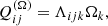
The non-diffusive stress corresponding to the Λ effect is then
 (6)
(6)
which can be extracted from a single experiment because off-diagonal components of  vanish. The horizontal, meridional, and vertical components of the Λ effect are given by
 (7)
(7)
 (8)
(8)
 (9)
(9)
where νt0 is a reference value of turbulent viscosity. The factor νt0Ω is used for normalization, whereas V, H, and M are dimensionless position-dependent functions.
It is important to bear in mind that Eqs. (7)–(9) are parametrisations derived from symmetry properties but do not specify the physical origin of the stress. Furthermore, Eqs. (7)–(9) are not limited to low Reynolds numbers as the results derived under the first-order smoothing approximation (FOSA) are.
3. The model
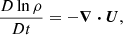
The model is the same as in several earlier studies (e.g. Käpylä 2024, and references therein). The equations for compressible hydrodynamics,
 (10)
(10)
 (11)
(11)
![Mathematical equation: $$ \begin{aligned} T \frac{D s}{D t}&= -\frac{1}{\rho } \left[\boldsymbol{\nabla } \boldsymbol{\cdot } \left(\boldsymbol{F}_{\rm rad} + \boldsymbol{F}_{\rm SGS}\right) + \mathcal{C} \right] + 2 \nu \boldsymbol{\mathsf{S }}^2, \end{aligned} $$](/articles/aa/full_html/2026/08/aa59779-26/aa59779-26-eq20.gif) (12)
(12)
were solved, where D/Dt = ∂/∂t + U⋅∇ is the advective derivative, ρ is the density, U is the velocity,  is the acceleration due to gravity with g > 0, p is the pressure, ν is the constant kinematic viscosity, S is the traceless rate-of-strain tensor with
  and Ω = Ω0(− sin θ, 0, cos θ)T is the rotation vector, where θ is the angle between Ω and g. T is the temperature, s is the specific entropy, Frad and FSGS are the radiative and turbulent sub-grid scale (SGS) fluxes, respectively, and 𝒞 describes surface cooling. The gas is assumed to be optically thick and fully ionised such that radiation is modelled via diffusion approximation. The ideal gas equation of state,
  applies, where ℛ is the gas constant, and cP and cV are the specific heats at constant pressure and volume, respectively. The radiative flux is Frad = −K∇T, where K is the radiative heat conductivity given by K = 16σSBT3/(3κρ); here, σSB is the Stefan-Boltzmann constant and κ is the opacity. Kramers opacity law, κ = κ0(ρ/ρ0)a(T/T0)b, with a = 1 and b = −7/2 was used (Weiss et al. 2004); see also Edwards (1990), Brandenburg et al. (2000), and Dorch & Nordlund (2001) for early applications to convection simulations.
Turbulent SGS diffusivity is applied for the entropy fluctuations with FSGS = −ρTχSGS∇s′, where  and the overbar indicates horizontal averaging. χSGS is constant throughout the domain and
  because the SGS diffusivity operates on the entropy fluctuations. The surface cooling is given by
  , where
  is a cooling timescale; T = e/cV is the temperature where e is the internal energy; and Tcool = Ttop corresponds to the fixed value at the upper boundary. Horizontal averages of horizontal flows
  and
and  were calculated at every time step and removed from the velocity field, so at all times we had U = u. The effects of mean flow removal are discussed in Appendix A.
3.1. Geometry, initial, and boundary conditions
The computational domain is a rectangular box where zbot ≤ z ≤ ztop is the vertical coordinate, with zbot/d = −0.45, ztop/d = 1.05, and where d is the depth of the initially isentropic layer (see below). The horizontal coordinates x and y are given by −2d ≤ (x, y)≤2d. The initial stratification consists of three layers. The two lower layers are polytropic, with the polytropic indices n1 = 3.25 (zbot/d ≤ z/d < 0) and n2 = 1.5 (0 ≤ z/d ≤ 1). The uppermost layer above z/d = 1 is initially isothermal. The initial velocity follows a Gaussian-noise distribution with amplitude of the order of  .
.
The horizontal boundaries are periodic. The vertical boundaries are impenetrable and stress-free for the flow, such that Ux, z = Uy, z = Uz = 0. The temperature gradient at the bottom boundary is given by ∂zT = −Fbot/Kbot, where Fbot is the fixed input flux and Kbot(x, y, zbot) is the heat conductivity at z = zbot. A constant temperature of T = Ttop was assumed on the top boundary.
3.2. Units, control parameters, and simulation strategy
The units of length, time, density, and entropy are given by [x]=d, ![Mathematical equation: $ [t] = \sqrt{d/g} $](/articles/aa/full_html/2026/08/aa59779-26/aa59779-26-eq31.gif) , [ρ]=ρ0, [s]=cP, where ρ0 is the initial value of density at z = ztop. The profile f(z) = 1 above z/d = 1 and f(z) = 0 below z/d = 1, connecting smoothly over a width of 0.025d, and
, [ρ]=ρ0, [s]=cP, where ρ0 is the initial value of density at z = ztop. The profile f(z) = 1 above z/d = 1 and f(z) = 0 below z/d = 1, connecting smoothly over a width of 0.025d, and  sets the initial pressure scale height at the surface. The Prandtl number based on the radiative heat conductivity is Pr(x, t) = ν/χ(x, t), where χ(x, t) = K(x, t)/cPρ(x, t). SGS Prandtl number is given by PrSGS = ν/χSGS.
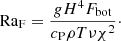
The Rayleigh number based on the energy flux is given by
 (13)
(13)
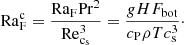
A diffusion-free Rayleigh number can be constructed using Recs = csH/ν, via
 (14)
(14)
Assuming H = HT ≡ cPT/g,  reduces to the dimensionless normalised flux (e.g. Brandenburg et al. 2005):
 (15)
(15)
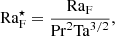
In rotating simulations, a flux-based, diffusion-free modified Rayleigh number is given by (e.g. Christensen 2002; Christensen & Aubert 2006; Käpylä 2024)
 (16)
(16)
where Ta = 4Ω02d4/ν2 is the Taylor number. This can be recast into a flux-based Coriolis number (Käpylä 2024; Bekki 2025):
 (17)
(17)
with u★ ≡ (Fbot/ρ)1/3 and H = HT.
In addition to explicit diffusion terms, the advective terms in Eqs. (10)–(12) are written in terms of a fifth-order upwinding derivative with a hyperdiffusive sixth-order correction with a flow-dependent diffusion coefficient; see Appendix B of Dobler et al. (2006). The PENCIL CODE1 was used to produce the simulations (Pencil Code Collaboration 2021).
3.3. Diagnostics quantities
The global Reynolds, SGS Péclet, and Coriolis numbers,
 (18)
(18)
describe the importance of viscosity, SGS diffusion, and rotation relative to advection, respectively. Here, urms is the volume averaged rms velocity and k1 = 2π/d is an estimate of the largest eddies in the system. Typically, we find χ ≪ χSGS in the convection zone in the current simulations.
The overall anisotropy of the flow is characterised by the parameters
 (19)
(19)
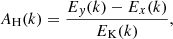
where Q = TrQij. The parameters AV and AH do not provide any information about the scale dependence of anisotropy. This is revealed by spectral anisotropy parameters, which are based on the power spectra of velocity components (e.g. Käpylä 2019a):
 (20)
(20)
 (21)
(21)
where ui2 = ∫Ei(k)dk, and EK(k) = ∑iEi(k). Diagnostics are time-averaged over the statistically steady part of the simulations, and horizontal or volume averages are additionally applied. Error estimates are given as the mean error of the mean where the number of turnover times is taken as the number of realisations.
4. Results
Some of the current slowly rotating runs use saturated snapshots of the progenitor Run K3h from Käpylä (2019c) as initial conditions, whereas several sets of runs were run from scratch. In total, eight sets of runs with a different CoF and seven runs corresponding to different values of θ were made; see Table 1.
Summary of the runs.
4.1. Description of the flow fields
Figure 1 shows representative flow fields from runs with slow (Set B), intermediate (Set E), and rapid rotation (Set H), highlighting the transition from cellular convection at slow rotation to columnar convection at rapid rotation. The effects of rotation are not apparent in the most slowly rotating cases at any latitude; see the left column of Fig. 1. For intermediate rotation the average size of convection cells somewhat reduced, and alignment of the convection cells with the rotation vector is discernible at the equator; see the middle column of Fig. 1. For rapid rotation the convection cells are significantly smaller and strongly aligned with the rotation vector; see right column of Fig. 1. This is particularly apparent at the equator (θ = 90°, Run H7), where structures are aligned with the x direction. The dominant size of convective structures at the pole (θ = 0°) was shown to follow the Coriolis-inertial-Archimedean (CIA) scaling, ℓ ∝ Co−1/2, in an earlier study (Käpylä 2024). A similar result was found for the equator (θ = 90°), corresponding here to Runs B7, E7, and H7 – shown in the bottom row of Fig. 1 – for spectra taken in the longitudinal (y) direction in Bekki (2025). The evident horizontal anisotropy is a key ingredient leading to the non-zero Λ effect.
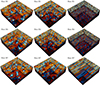 |
Fig. 1. Flow fields from Runs B1, B4, and B7 with CoF ≈ 0.55 (left column), Runs E1, E4, and E7 with CoF ≈ 4.5…4.9 (middle), and from Runs H1, H4, and H7 with CoF ≈ 12…17 (right) at latitudes θ = 0° (top row), θ = 45° (middle), and θ = 90° (bottom). |
4.2. Anisotropy of turbulence
The vertical and horizontal Λ effects are, to the lowest order, proportional to the turbulence anisotropies given by AV and AH, respectively (e.g. Rüdiger 1980). Representative results for AV and AH from runs with slow (Set B), intermediate (Set E), and rapid rotation (Set H) are shown in Fig. 2. In the slowly rotating cases, AV is negative throughout the convection zone, similarly to non-rotating cases (not shown). For CoF ≈ 0.55 (Set B) the vertical anisotropy, AV, remains practically constant in the upper part of the convection zone (z/d ≳ 0.65) as a function of latitude. The absolute value of AV decreases slightly in the lower part of the convection zone from the pole towards the equator. For intermediate (Set E) and rapid rotation (Set H) the latitudinal variation of AV increases; see panels (b) and (c) of Fig. 2. AV generally decreases from the pole to the equator. In the most rapidly rotating cases, AV at the equator is again somewhat higher than in the low-latitude cases; see panel (c) of Fig. 2. Furthermore, while AV at the pole decreases for intermediate rotation, it is enhanced in the rapidly rotating cases.
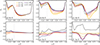 |
Fig. 2. Anisotropy parameters AV (top row) and AH (bottom) from runs in Set B with CoF ≈ 0.55 (left), Set E with CoF ≈ 4.5…4.9 (middle), and from Set H with CoF ≈ 12…17 (right). |
The horizontal anisotropy AH is much weaker than AV for slow rotation because it is induced by rotation, while the latter is partly an inherent property of convection. AH vanishes at the pole due to symmetry and increases monotonically towards the equator for slow and intermediate rotation; see panels (d) and (e) of Fig. 2. AH is negative for rapid rotation (Set H; see panel (f) of Fig. 2), which to the lowest order would imply poleward angular momentum transport that promotes anti-solar differential rotation (e.g. Rüdiger 1980). However, the latter result is valid for slow rotation corresponding to Co ≪ 1, which is not satisfied in the current rapidly rotating runs. Furthermore, this argument relies only on the magnitude of AV, while spatial scales of the horizontal flows are also very different in the latitudinal (x) and longitudinal (y) directions; see Fig. 1.
To study the anisotropy in more detail, a spectral decomposition was made; see Eqs. (20) and (21). Representative results for AV(k) and AH(k) are shown in Figs. 3 and 4. Large scales are dominated by horizontal flows such that AV(k) > 0, similarly to the non-rotating case (not shown). The zero-crossing of AV(k) occurs at a progressively higher normalised wave number of  as the rotation rate increases. The negative AV(k) at intermediate and large wave numbers are responsible for AV = ∫AV(k)dk < 0 in the bulk of the convection zone in all cases. For slow rotation (Runs E[1,4,7]) AV(k) does not change appreciably as a function of θ, whereas for the intermediate and rapid rotation runs the crossover from positive to negative AV(k) occurs at a lower wave number; see the middle and right panels of Fig. 3.
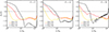 |
Fig. 3. Anisotropy parameter AV(k) from runs with slow (Runs B1, B4, and B7), intermediate (Run E1, E4, and E7), and rapid rotation (Run H1, H4, and H7) at θ = 0° (left panel), θ = 45° (middle), and θ = 90° (right), respectively, near the middle of the convection zone at z/d = 0.49. |
As discussed above, the horizontal anisotropy becomes prominent only at rapid rotation, and it vanishes for θ = 0°; see Fig. 4. For slow and intermediate rotation the main contribution to the overall positive AH comes from large and intermediate scales; see the middle and right panels of Fig. 4. This can be understood as a consequence of rotational alignment of the largest convection cells that have the greatest Coriolis numbers. In the rapid rotation regime a similar trend is seen on large scales, but the behaviour for  of the latitudinal (x) component dominates, leading to AH = ∫AHkdk < 0.
Turbulence becomes quasi-two-dimensional for sufficiently rapid rotation leading to diminishing velocity along Ω (e.g. Müller & Thiele 2007). Strong density stratification has a similar effect along the direction of the gravitational acceleration (e.g. Boffetta 2023). The latter has been adopted as one of the building blocks for theories of angular momentum transport in stellar convection zones (e.g. Kitchatinov & Rüdiger 1993). This approach was generalised by Kitchatinov & Rüdiger (2005), the authors of which introduced an anisotropy parameter, a, that characterises the difference between vertical and horizontal motions in the unperturbed case; see their Eq. A14. Assuming for simplicity that the scale ratio ℓcorr2/L2 = 1, the vertical anisotropy parameter, AV, can be written in terms of a as follows:
 (22)
(22)
such that  corresponds to isotropy. The range of AV in Fig. 3 inside the convection zone is roughly −0.2 to −1.2, corresponding to a = 3.5…8.5, which is significantly higher than the values typically used in mean-field approaches (e.g. Kitchatinov & Rüdiger 2005; Pipin & Kosovichev 2018).
4.3. Reynolds stress and Λ effect
Horizontally and temporally averaged off-diagonal Reynolds stresses are shown in Fig. 5. The stresses are assumed to be due to non-diffusive origin, and are attributed here to the Λ effect since horizontally averaged mean flows have been suppressed in the present simulations. The horizontal stress, Qxy, is responsible for generating horizontal or latitude-dependent differential rotation in spherical coordinates. Qxy is on average positive almost everywhere corresponding to equatorward flux of angular momentum; see the left column of Fig. 5. For the slowest rotation rates the data are not sufficiently converged to rule out negative values, which, however, are theoretically expected only in cases where shear is retained (Rüdiger et al. 2019). As the rotation rate is increased, the horizontal stress is increasingly concentrated near the equator; see the data for Sets E to H in the four bottom left panels of Fig. 5. This behaviour is commonly seen in f-plane simulations (e.g. Chan 2001; Käpylä et al. 2004; Hupfer et al. 2005) of convection but not in corresponding forced turbulence calculations (e.g. Käpylä & Brandenburg 2008; Käpylä 2019b). The main difference between the forced turbulence and convection set-ups is the lack of stratification and thermodynamics in the former such that, for example, thermal Rossby waves are not excited. Convective structures corresponding to the latter are the main contributor to Qxy near the equator (see also Käpylä et al. 2011a). On the other hand, global convection simulations do not show a similar concentration of horizontal stress (Qθϕ) near the equator (e.g. Käpylä et al. 2011a). This is likely explained by the differences in geometry; in the current set-up the horizontal stress cannot generate a mean flow in the horizontally averaged sense because of the horizontal periodicity of the domain, whereas in global simulations the divergence of Qθϕ leads to a mean flow. However, it is possible to generate mean flows that depend on x or y but vanish under a horizontal average even in the present geometry, although this has not been observed in the current simulations. A possible reason is that the horizontal size of the domain is too small or that the horizontal aspect ratio of the domain needs to be unequal to unity, which effectively introduces a preferred direction (e.g. Guervilly & Hughes 2017; Currie et al. 2020). Furthermore, the formation of large-scale vortices (e.g. Chan 2007; Käpylä et al. 2011b; Guervilly et al. 2014) was not observed in the current simulations, most likely because the fluid Reynolds number is too low; see the discussion in Käpylä (2024).
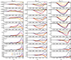 |
Fig. 5. Off-diagonal Reynolds stresses |


The meridional stress, Qxz, does not directly participate in the angular momentum transport, but it has an indirect influence via the meridional flow. This component is predominantly negative for slow rotation (Co ≲ 0.25, Sets A to C), with a magnitude similar to Qxy. For Co ≳ 0.6, Qxz first changes sign for θ = 75° and, at even more rapid rotation, for θ = 60°. This is in contrast to earlier forced turbulence simulations, which also yielded Qxz < 0 for rapid rotation (e.g. Käpylä 2019b). It is possible that the difference is also due to the thermal Rossby waves that were absent in the isothermal forced turbulence models. The magnitude of Qxz is less than the other off-diagonal components for Co ≳ 0.6. The impact of this stress component for stellar differential rotation has not been studied in detail.
The vertical stress Qyz generates radial differential rotation. For slow rotation (Co ≲ 0.6) Qyz is negative almost everywhere and roughly proportional to Ω. This agrees with analytic results and forced turbulence simulations (e.g. Käpylä & Brandenburg 2008; Käpylä 2019b). However, at sufficiently rapid rotation the sign of Qyz changes near the equator where large positive values are observed; see the data for Sets F to H in the middle column of Fig. 5. This feature is absent in isothermal forced turbulence models and is due to thermal Rossby waves that are excited in rotating convection (e.g. Busse 2002). Analyses of the radial stress Qrϕ – corresponding to Qyz in the current Cartesian geometry – in spherical shells and wedges have shown that the large-scale convective modes associated with the thermal Rossby waves produce the dominant contribution to Qrϕ and produce equatorial acceleration (e.g. Käpylä 2023). This is in contrast to some hydrodynamic mean-field models, where the radial stress vanishes for rapid rotation and equatorial acceleration is achieved via equatorward horizontal flux of angular momentum (e.g. Kitchatinov 2013).
The non-diffusive Reynolds stresses from Eqs. (7) to (9) can be represented in terms of the Λ-effect coefficients as
 (23)
(23)
 (24)
(24)
 (25)
(25)
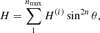
where 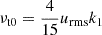 was used, and where the tilde refers to normalisation by urms2. The functional form of νt0 is taken for a non-rotating case from the analytic study of Kitchatinov et al. (1994). Results from numerical simulations of isotropically forced homogeneous turbulence tend to be somewhat higher; see Käpylä et al. (2020). Therefore, the choice of νt0 in the normalisation leads to some uncertainty in the absolute values of the coefficients. We followed the same procedure as in Käpylä (2019b) and expanded the coefficients in powers of sin2θ
 (26)
(26)
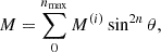 (27)
(27)
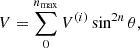 (28)
(28)
where H(0) is assumed to vanish due to symmetry. The Reynolds stresses vary as a function of height, but here we applied volume averaging, denoted by angle brackets ⟨.⟩ over the 0 ≤ z/d ≤ 1 range to simplify the analysis. The coefficients V, H, and M were fitted with up to nmax = 3 using Eqs. (23)–(25) and Eqs. (26)–(28) with volume-averaged numerical data for the Reynolds stresses. The fit was deemed accurate enough when the mean error of the mean between the numerical data and the reconstruction with the fitted coefficients did not decrease by more then ten per cent when an additional coefficient was taken into account. However, an nmax higher than three would be needed to fit the vertical stress  for the most rapidly rotating cases (Sets G and H), but this was not pursued. The numerical data as well as the fits are shown in Fig. 6 for all runs. Furthermore, Table 2 summarises the fitted coefficients.
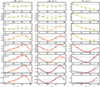 |
Fig. 6. Volume and time-averaged Λ coefficients ⟨ℋ⟩ (left panels), ⟨ℳ⟩ (middle), and ⟨𝒱⟩ (right) from all sets of runs along with best fits to Eqs. (28)–(27). The thick lines show an adequate fit according to the criteria in the text, and the thin lines show fits with one fewer coefficient for comparison. The colours denote the maximum number of coefficients, nmax, taken into account in the fits such that nmax = 0, 1, 2, and 3 correspond to yellow, orange, red, and purple, respectively. |
Summary of the fitted Λ coefficients.
The horizontal Λ effect is positive for all rotation rates, although in the slowest rotation cases studied (Sets A, B, and C) the results are not statistically significant. These results are in accordance with quasi-linear theory (e.g. Rüdiger 1989), where negative values of ℋ are expected only when large-scale flows (Rüdiger et al. 2019) or magnetic fields (e.g. Kitchatinov & Rüdiger 2004; Käpylä 2019b) are present, both of which are absent in the current simulations. The concentration of the horizontal stress near the equator is reflected in the horizontal Λ effect coefficient, ℋ, although this behaviour is subdued in Fig. 6 due to the volume averaging. Nevertheless, ⟨ℋ⟩ tends to be at its maximum at the nearest latitude away from the equator for Co > 0.6 (Sets E to H). This is reflected by the need to use coefficients up to H(3) to already fit the data in Set E; see the second to fourth columns of Table 2. More data points at lower latitudes would be needed to determine the full latitude profile, but this is out of the scope of the present study. In Käpylä (2019b) all of the H(i) coefficients were found to be positive, which is not the case for H(1) in the present study.
The volume-averaged meridional Λ effect, ⟨ℳ⟩, shown in the middle column of Fig. 6, is negative for slow rotation up to around Co = 0.25 (Set C). For more rapid rotation, ⟨ℳ⟩ changes sign near the equator which was not observed in the forced turbulence simulations of Käpylä (2019b), but was present in earlier simulations by Käpylä & Brandenburg (2008). Pulkkinen et al. (1993)2 reported M(0) = −0.03 and M(1) = 0.06, although the quality of their fit is rather modest; see their Fig. 11. The signs coincide with the current Set C, although the values are greater than in the current runs. This is possibly because mean flows were retained in the runs of Pulkkinen et al. (1993) that also contribute to the Reynolds stress; (see e.g. Rüdiger et al. 2019). For more rapid rotation (Sets D onwards), at least three coefficients are needed to fit the data. The sign of M(0) coincides with that in forced turbulence simulations of Käpylä (2019b), but the behaviour of the higher order coefficients is more complex.
The vertical Λ effect, ⟨𝒱⟩, is negative for for CoF ≲ 4.56 (Sets A to E). In the two slowest rotating sets A and B, only the fundamental mode of the Λ effect, described by V(0) is needed to fit the numerical data; see Table 2. The absolute value of V(0) is of the order of 0.05 in the slowest rotation cases. The sign and functional form agree with forced turbulence simulations (e.g. Käpylä 2019b; Barekat et al. 2021), but the absolute value is an order of magnitude smaller in the current results although the vertical anisotropy of the flow as measured by ΛV is similar in both cases; compare Fig. 2 with Fig. 3 of Barekat et al. (2021). For Co ≳ 2.5 (Sets F to H), the sign of ⟨𝒱⟩ changes near the equator. In the current results V(0) < 0 and V(3) > 0 everywhere, whereas V(1) > 0 and V(2) < 0, apart from in Set E; see the three last columns in Table 2. In Käpylä (2019b), V(0) is also predominantly negative, whereas V(1) < 0 and V(2) > 0 in contrast to the current results. Analytic studies do not typically consider coefficients higher than V(1); see, for example, Kitchatinov & Rüdiger (2005), Pipin & Kosovichev (2018).
The qualitative differences between the analytic theories and isothermal forced turbulence simulations in comparison to the current results for the vertical Λ effect are likely due to the dominating influence of thermal Rossby waves that appear as tilted columnar convection cells near the equator (e.g. Käpylä 2023). Thermal Rossby waves are typically not captured by analytics that rely on simplified turbulence models, and therefore a positive ⟨𝒱⟩ for rapid rotation is absent in such theories. This often also applies to analytic theories where the convective heat flux is taken into account (e.g. Kleeorin & Rogachevskii 2006); see, however Rogachevskii & Kleeorin (2018). Yet, Pipin & Kosovichev (2018) found that the standard mean-field theory does yield a sign change of the vertical Λ effect for rapid rotation when the spatial non-uniformity of the convective turnover time is taken into account.
5. Conclusions
The current simulations show that the radial, non-diffusive angular momentum transport, parameterised by the vertical Λ effect, is negative for slow rotation (Co ≲ 1.3) in rotating density-stratified convection. The horizontal Λ effect is positive, corresponding to equatorward angular momentum flux, for all rotation rates. These findings are in qualitative agreement with isothermal forced turbulence simulations (e.g. Käpylä & Brandenburg 2008; Käpylä 2019b; Barekat et al. 2021) and analytic mean-field theories (e.g. Kitchatinov & Rüdiger 1995; Kleeorin & Rogachevskii 2006). For more rapid rotation the radial Λ effect changes sign, and the horizontal flux is increasingly concentrated at low latitudes. The change of sign of of the vertical Λ effect is due to the emergence of prograde propagating thermal Rossby waves, which are not accounted for in analytic theories of angular momentum transport (e.g. Rüdiger 1989; Kitchatinov & Rüdiger 2005). In global convection simulations the thermal Rossby waves are the cause of solar-like differential rotation. On the other hand, thermal Rossby waves have not been observed in the Sun (e.g. Birch et al. 2024, and references therein), and if they are present, they must be much weaker than in simulations. Therefore, the origin of solar and stellar differential rotation is related to the ongoing debate regarding the nature of convection in the Sun (e.g. Schumacher & Sreenivasan 2020; Hotta et al. 2023, and references therein), often referred to as the convective conundrum (e.g. O’Mara et al. 2016).
The current study probes the hydrodynamic regime with simulations where the density stratification is much weaker than in stars and where the transition to optically thin photosphere is modelled rather crudely. Magnetic fields have been shown to strongly affect the angular momentum transport and large-scale flows in global simulations (e.g. Hotta et al. 2022; Hotta 2025; Käpylä 2023; Soderlund et al. 2025). Magnetic fields have also been shown to significantly influence the Λ effect in theoretical and idealised numerical studies (e.g. Kitchatinov & Rüdiger 2004; Käpylä 2019b,a). The inability to incorporate a realistic stratification or proper radiative surface possibly inhibits non-local entropy rain (e.g. Spruit 1997; Brandenburg 2016; Käpylä 2025) in current studies. The effects on convective angular momentum transport of these aspects need to be addressed in future studies.
Acknowledgments
I thank the anonymous referee, Valery Pipin, and Igor Rogachevskii for their comments on the manuscript. The simulations were performed using the resources granted by the Gauss Center for Supercomputing for the Large-Scale computing project “Cracking the Convective Conundrum” in the Leibniz Supercomputing Centre’s SuperMUC-NG supercomputer in Garching, Germany. This work was supported in part by the Deutsche Forschungsgemeinschaft Heisenberg programme (grant No. KA 4825/4-1).
References
- Aurnou, J., Heimpel, M., & Wicht, J. 2007, Icarus, 190, 110 [NASA ADS] [CrossRef] [Google Scholar]
- Barekat, A., Käpylä, M. J., Käpylä, P. J., Gilson, E. P., & Ji, H. 2021, A&A, 655, A79 [NASA ADS] [CrossRef] [EDP Sciences] [Google Scholar]
- Bekki, Y. 2025, A&A, 703, A262 [Google Scholar]
- Birch, A. C., Proxauf, B., Duvall, T. L., et al. 2024, Phys. Fluids, 36, 117136 [Google Scholar]
- Boffetta, G. 2023, Atmosphere, 14, 1688 [Google Scholar]
- Brandenburg, A. 2016, ApJ, 832, 6 [Google Scholar]
- Brandenburg, A., Nordlund, A., & Stein, R. F. 2000, in Geophysical and Astrophysical Convection, eds. P. A. Fox, & R. M. Kerr, 85 [Google Scholar]
- Brandenburg, A., Chan, K. L., Nordlund, Å., & Stein, R. F. 2005, AN, 326, 681 [NASA ADS] [Google Scholar]
- Busse, F. H. 2002, Phys. Fluids, 14, 1301 [NASA ADS] [CrossRef] [Google Scholar]
- Chan, K. L. 2001, ApJ, 548, 1102 [Google Scholar]
- Chan, K. L. 2007, Astron. Nachr., 328, 1059 [Google Scholar]
- Christensen, U. R. 2002, J. Fluid Mech., 470, 115 [NASA ADS] [CrossRef] [Google Scholar]
- Christensen, U. R., & Aubert, J. 2006, Geophys. J. Int., 166, 97 [NASA ADS] [CrossRef] [Google Scholar]
- Currie, L. K., Barker, A. J., Lithwick, Y., & Browning, M. K. 2020, MNRAS, 493, 5233 [CrossRef] [Google Scholar]
- Dobler, W., Stix, M., & Brandenburg, A. 2006, ApJ, 638, 336 [NASA ADS] [CrossRef] [Google Scholar]
- Dorch, S. B. F., & Nordlund, Å. 2001, A&A, 365, 562 [Google Scholar]
- Edwards, J. M. 1990, MNRAS, 242, 224 [NASA ADS] [CrossRef] [Google Scholar]
- Guervilly, C., & Hughes, D. W. 2017, Phys. Rev. Fluids, 2, 113503 [Google Scholar]
- Guervilly, C., Hughes, D. W., & Jones, C. A. 2014, J. Fluid Mech., 758, 407 [Google Scholar]
- Hotta, H. 2025, ApJ, 985, 163 [Google Scholar]
- Hotta, H., Kusano, K., & Shimada, R. 2022, ApJ, 933, 199 [NASA ADS] [CrossRef] [Google Scholar]
- Hotta, H., Bekki, Y., Gizon, L., Noraz, Q., & Rast, M. 2023, Space Sci. Rev., 219, 77 [NASA ADS] [CrossRef] [Google Scholar]
- Hupfer, C., Käpylä, P., & Stix, M. 2005, Astron. Nachr., 326, 223 [Google Scholar]
- Käpylä, P. J. 2019a, Astron. Nachr., 340, 744 [CrossRef] [Google Scholar]
- Käpylä, P. J. 2019b, A&A, 622, A195 [NASA ADS] [CrossRef] [EDP Sciences] [Google Scholar]
- Käpylä, P. J. 2019c, A&A, 631, A122 [NASA ADS] [CrossRef] [EDP Sciences] [Google Scholar]
- Käpylä, P. J. 2023, A&A, 669, A98 [NASA ADS] [CrossRef] [EDP Sciences] [Google Scholar]
- Käpylä, P. J. 2024, A&A, 683, A221 [NASA ADS] [CrossRef] [EDP Sciences] [Google Scholar]
- Käpylä, P. J. 2025, A&A, 698, L13 [NASA ADS] [CrossRef] [EDP Sciences] [Google Scholar]
- Käpylä, P. J., & Brandenburg, A. 2008, A&A, 488, 9 [Google Scholar]
- Käpylä, P. J., Korpi, M. J., & Tuominen, I. 2004, A&A, 422, 793 [NASA ADS] [CrossRef] [EDP Sciences] [Google Scholar]
- Käpylä, P. J., Mantere, M. J., Guerrero, G., Brandenburg, A., & Chatterjee, P. 2011a, A&A, 531, A162 [NASA ADS] [CrossRef] [EDP Sciences] [Google Scholar]
- Käpylä, P. J., Mantere, M. J., & Hackman, T. 2011b, ApJ, 742, 34 [CrossRef] [Google Scholar]
- Käpylä, P. J., Rheinhardt, M., Brandenburg, A., & Käpylä, M. J. 2020, A&A, 636, A93 [NASA ADS] [CrossRef] [EDP Sciences] [Google Scholar]
- Kitchatinov, L. L. 2013, in Solar and Astrophysical Dynamos and Magnetic Activity, eds. A. G. Kosovichev, E. de Gouveia Dal Pino, & Y. Yan, 294, 399 [Google Scholar]
- Kitchatinov, L. L., & Rüdiger, G. 1993, A&A, 276, 96 [Google Scholar]
- Kitchatinov, L. L., & Rüdiger, G. 1995, A&A, 299, 446 [NASA ADS] [Google Scholar]
- Kitchatinov, L. L., & Rüdiger, G. 2004, Astron. Nachr., 325, 496 [NASA ADS] [CrossRef] [Google Scholar]
- Kitchatinov, L. L., & Rüdiger, G. 2005, Astron. Nachr., 326, 379 [NASA ADS] [CrossRef] [Google Scholar]
- Kitchatinov, L. L., Pipin, V. V., & Rüdiger, G. 1994, Astron. Nachr., 315, 157 [NASA ADS] [CrossRef] [Google Scholar]
- Kleeorin, N., & Rogachevskii, I. 2006, Phys. Rev. E, 73, 046303 [Google Scholar]
- Mori, K., & Hotta, H. 2023, MNRAS, 519, 3091 [Google Scholar]
- Müller, W.-C., & Thiele, M. 2007, EPL, 77, 34003 [Google Scholar]
- O’Mara, B., Miesch, M. S., Featherstone, N. A., & Augustson, K. C. 2016, Adv. Space Res., 58, 1475 [CrossRef] [Google Scholar]
- Pencil Code Collaboration (Brandenburg, A., et al.) 2021, J. Open Source Softw., 6, 2807 [Google Scholar]
- Pipin, V. V., & Kosovichev, A. G. 2018, ApJ, 854, 67 [Google Scholar]
- Pulkkinen, P., Tuominen, I., Brandenburg, A., Nordlund, A., & Stein, R. F. 1993, A&A, 267, 265 [NASA ADS] [Google Scholar]
- Reinhold, T., & Gizon, L. 2015, A&A, 583, A65 [NASA ADS] [CrossRef] [EDP Sciences] [Google Scholar]
- Rogachevskii, I., & Kleeorin, N. 2018, J. Plasma Phys., 84, 735840201 [Google Scholar]
- Rüdiger, G. 1980, Geophys. Astrophys. Fluid Dynam., 16, 239 [Google Scholar]
- Rüdiger, G. 1989, Differential Rotation and Stellar Convection. Sun and Solar-type Stars (Berlin: Akademie Verlag) [Google Scholar]
- Rüdiger, G., & Küker, M. 2021, A&A, 649, A173 [Google Scholar]
- Rüdiger, G., Egorov, P., & Ziegler, U. 2005, Astron. Nachr., 326, 315 [Google Scholar]
- Rüdiger, G., Kitchatinov, L. L., & Hollerbach, R. 2013, Magnetic Processes in Astrophysics: Theory, Simulations, Experiments (Wiley-VCH) [Google Scholar]
- Rüdiger, G., Küker, M., Käpylä, P. J., & Strassmeier, K. G. 2019, A&A, 630, A109 [EDP Sciences] [Google Scholar]
- Schumacher, J., & Sreenivasan, K. R. 2020, Rev. Mod. Phys., 92, 041001 [NASA ADS] [CrossRef] [Google Scholar]
- Soderlund, K. M., Wulff, P., Käpylä, P. J., & Aurnou, J. M. 2025, MNRAS, 541, 1816 [Google Scholar]
- Spruit, H. 1997, Mem. Soc. Astron. It., 68, 397 [Google Scholar]
- Weiss, A., Hillebrandt, W., Thomas, H.-C., & Ritter, H. 2004, Cox and Giuli’s Principles of Stellar Structure (Cambridge, UK: Cambridge Scientific Publishers Ltd) [Google Scholar]
Their M(i) corresponds to M(i − 1) of the current study.
Appendix A: Effects of mean flow removal
According to Eq. (2) the Reynolds stress can be decomposed to contributions from the background turbulence, rotation, and shear. In practice this is complicated by the inherent non-linearity of the Navier-Stokes equations. For example, sufficiently strong shear leads to production of turbulence; see e.g. Käpylä et al. (2020). Removing shear flows is therefore also likely to affect the solutions. Here we consider a few otherwise identical simulations where the mean flows are either a part of the solution or where they are removed. The latter correspond to the runs listed in Table 1.
We use two diagnostics to study the effect of mean flow removal, which are the overall velocity amplitude urms and the horizontally averaged off-diagonal Reynolds stress component Qyz. These are shown for four representative runs in Fig. A.1. The change of the volume-averaged rms velocity reflects the strength of the removed mean flows. The mean flows in the slowly rotating Run D6 are relatively strong due to which the rms-velocity is decreased by roughly 5 per cent. The clearest effect is seen at the equator (Run F7), where strong mean flows are generated and their removal leads to a decrease of the flow amplitude by about 20 per cent. Mean flows in runs at higher latitudes and faster rotation tend to be weaker; see the data for Runs F4 and H5. These results regarding mean flows are in accordance with earlier studies (e.g. Chan 2001; Käpylä et al. 2004). Similarly the Reynolds stresses are modified by the absence of mean flows because the diffusive contribution to the stress is absent. This effect is again strongest in cases with larger mean flows as indicated by the lower panel of Fig. A.1. Assuming that the turbulent viscosity νt is positive and because  in Run D6, we would expect the diffusive contribution to the stress to be positive, that is
  . This agrees with the results of the current simulations; see the black lines in the lower panel of Fig. A.1. In Runs F4 and H5 the differences between the runs with and without shear are small and not always suggestive of a positive νt. This can be due to insufficient statistical convergence. The results of Run F7, where Qyz should vanish in the case where the mean flows are retained (e.g. Bekki 2025) are suggestive of this. The non-zero residual (red solid line) in the lower panel of Fig. A.1 can be used as an estimate of the statistical uncertainty of the results.
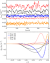 |
Fig. A.1. Volume-averaged rms velocity urms/(dg)1/2 as a function of time (upper panel) and Reynolds stress component Qyz/dg in units of 10−4 as a function of z (lower panel) from Runs D6 (dotted black line), F4 (dotted blue), F7 (dotted red), and H5 (dotted orange). The solid lines show the same quantities from corresponding runs where mean flows are retained. |
All Tables
All Figures
|
Fig. 1. Flow fields from Runs B1, B4, and B7 with CoF ≈ 0.55 (left column), Runs E1, E4, and E7 with CoF ≈ 4.5…4.9 (middle), and from Runs H1, H4, and H7 with CoF ≈ 12…17 (right) at latitudes θ = 0° (top row), θ = 45° (middle), and θ = 90° (bottom). |
| In the text | |
|
Fig. 2. Anisotropy parameters AV (top row) and AH (bottom) from runs in Set B with CoF ≈ 0.55 (left), Set E with CoF ≈ 4.5…4.9 (middle), and from Set H with CoF ≈ 12…17 (right). |
| In the text | |
|
Fig. 3. Anisotropy parameter AV(k) from runs with slow (Runs B1, B4, and B7), intermediate (Run E1, E4, and E7), and rapid rotation (Run H1, H4, and H7) at θ = 0° (left panel), θ = 45° (middle), and θ = 90° (right), respectively, near the middle of the convection zone at z/d = 0.49. |
| In the text | |
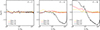 |
Fig. 4. Anisotropy parameter AH(k) for the same runs as in Fig. 3. |
| In the text | |
|
Fig. 5. Off-diagonal Reynolds stresses |
| In the text | |
|
Fig. 6. Volume and time-averaged Λ coefficients ⟨ℋ⟩ (left panels), ⟨ℳ⟩ (middle), and ⟨𝒱⟩ (right) from all sets of runs along with best fits to Eqs. (28)–(27). The thick lines show an adequate fit according to the criteria in the text, and the thin lines show fits with one fewer coefficient for comparison. The colours denote the maximum number of coefficients, nmax, taken into account in the fits such that nmax = 0, 1, 2, and 3 correspond to yellow, orange, red, and purple, respectively. |
| In the text | |
|
Fig. A.1. Volume-averaged rms velocity urms/(dg)1/2 as a function of time (upper panel) and Reynolds stress component Qyz/dg in units of 10−4 as a function of z (lower panel) from Runs D6 (dotted black line), F4 (dotted blue), F7 (dotted red), and H5 (dotted orange). The solid lines show the same quantities from corresponding runs where mean flows are retained. |
| In the text | |
Current usage metrics show cumulative count of Article Views (full-text article views including HTML views, PDF and ePub downloads, according to the available data) and Abstracts Views on Vision4Press platform.
Data correspond to usage on the plateform after 2015. The current usage metrics is available 48-96 hours after online publication and is updated daily on week days.
Initial download of the metrics may take a while.