


| Issue |
A&A
Volume 711, July 2026
|
|
|---|---|---|
| Article Number | A228 | |
| Number of page(s) | 9 | |
| Section | Planets, planetary systems, and small bodies | |
| DOI | https://doi.org/10.1051/0004-6361/202660674 | |
| Published online | 17 July 2026 | |
Atmospheric sputtering on Mars: roles of hydrogen energetic neutral atoms and precipitating solar wind protons
1
Planetary Environmental and Astrobiological Research Laboratory (PEARL), Sun Yat-Sen University,
Zhuhai,
Guangdong,
China
2
Institute of Science and Technology for Deep Space Exploration,
Nanjing University-Suzhou Campus,
Suzhou,
China
3
School of Space and Earth Sciences, Beihang University,
Beijing,
China
4
National Space Science Center, Chinese Academy of Sciences,
Beijing,
China
★ Corresponding author: This email address is being protected from spambots. You need JavaScript enabled to view it.
Received:
29
April
2026
Accepted:
25
June
2026
Abstract
Context. Atmospheric sputtering is a key nonthermal process that contributes to the escape of heavy species from Mars.
Aims. Using simultaneous observations from Tianwen-1 and MAVEN in December 2021, we quantified sputtering escape driven by precipitating solar wind protons and hydrogen energetic neutral atoms (ENAs).
Methods. A Monte Carlo model was employed to calculate sputtering yields and corresponding CO2 and O escape rates.
Results. Both species exhibit increasing yields with incident energy and incidence angle, as well as enhanced recoil production at higher altitudes. The simulations show that collisional thermalization strongly suppresses the escape of heavy recoils produced deep in the atmosphere, but that a small residual fraction of CO2 and O recoils can survive collisional filtering and escape. Precipitating protons and hydrogen ENAs are able to drive substantial CO2 and O escape rates on the order of 1022 s−1 . Compared with other loss channels, sputtering contributes 1022–1023 s−1 of C and O escape, which is less than photochemical loss but uniquely capable of ejecting heavy molecules such as CO2 and Ar.
Conclusions. The results indicate that proton- and ENA-induced sputtering persist as key and variable mechanisms shaping the longterm evolution of the Martian atmosphere.
Key words: planets and satellites: atmospheres / planets and satellites: terrestrial planets / planets and satellites: individual: Mars
© The Authors 2026
 Open Access article, published by EDP Sciences, under the terms of the Creative Commons Attribution License (https://creativecommons.org/licenses/by/4.0), which permits unrestricted use, distribution, and reproduction in any medium, provided the original work is properly cited.
This article is published in open access under the Subscribe to Open model. This email address is being protected from spambots. You need JavaScript enabled to view it. to support open access publication.
1 Introduction
Atmospheric escape has played a fundamental role in shaping the current state and long-term evolution of Mars (Lammer et al. 2013; Jakosky 2021). Geological and isotopic evidence indicates that early Mars likely possessed a much denser atmosphere, capable of sustaining surface liquid water, which could have supported a more habitable environment (e.g., Wordsworth 2016; Jakosky et al. 2017; Ramirez & Craddock 2018; Kite 2019). Over billions of years, however, the gradual loss of volatiles transformed Mars into the cold and arid planet we observe today. A variety of mechanisms have been proposed to account for this loss, including thermal escape, photochemical escape, ion pickup, bulk ion outflow, and atmospheric sputtering (Jakosky et al. 2018, and references therein), with the latter recognized as a particularly effective process. In this mechanism, incident high-energy particles collide with neutral atmospheric species, initiating cascades of secondary collisions, some of which transfer sufficient kinetic energy to allow particles to escape the planet’s gravitational potential Johnson (1994). Unlike other processes that predominantly affect light species, sputtering can eject heavier molecules, particularly CO2 and Ar, thereby significantly altering the atmospheric composition and enhancing atmospheric loss (e.g., Wang et al. 2014, 2015; Jakosky et al. 2017; Leblanc et al. 2018; Curry et al. 2025).
Despite its recognized importance, the quantitative contribution of sputtering to atmospheric escape on Mars remains uncertain. Early modeling studies suggested that sputtering could account for the removal of a substantial fraction of Mars’ ancient atmosphere (e.g., Luhmann et al. 1992; Johnson et al. 2000). More recent investigations, however, have reported widely varying escape rates, reflecting the strong sensitivity of sputtering escape to factors such as solar wind energy spectra, atmospheric density profiles, and adopted collision cross sections (e.g., Wang et al. 2014; Leblanc et al. 2018). A central unresolved issue is the identification of the dominant drivers of sputtering escape. While solar wind protons are generally considered the primary source of momentum transfer (e.g., Leblanc et al. 2018; Shematovich 2021), magnetosheath-heavy ions and energetic neutral atoms (ENAs) generated through charge exchange may also play critical roles under certain solar wind conditions (e.g., Fang et al. 2013; Ma et al. 2025).
It is important to distinguish these sputtering sources. Many previous studies have focused on sputtering driven by pickup O+ ions, which can transfer momentum more efficiently to heavy atmospheric species because of their larger masses and, in many cases, higher characteristic energies (e.g., Luhmann et al. 1992; Johnson et al. 2000; Leblanc et al. 2018). Such particles are therefore expected to be more effective in ejecting heavy species such as CO2 and Ar. By contrast, sputtering driven by precipitating solar wind protons and hydrogen ENAs represents a lighter but highly variable source that is directly linked to the solar wind interaction with Mars. The situation is further complicated by the highly variable interaction between the solar wind and the Martian magnetosphere: Mars’ induced magnetosphere is dynamic and strongly modulated by upstream solar wind conditions, giving rise to pronounced temporal and spatial variability in particle precipitation and sputtering efficiency (e.g., Dubinin et al. 2006; Brain et al. 2010; Wang et al. 2018). These uncertainties make it difficult to reconcile model predictions and to place robust constraints on the long-term contribution of sputtering to Martian atmospheric loss.
The simultaneous operation of China’s Tianwen-1 mission (Zou et al. 2021) and NASA’s Mars Atmosphere and Volatile Evolution (MAVEN) mission (Jakosky et al. 2015) provides an unprecedented opportunity to reduce these uncertainties and advance our understanding of sputtering escape on Mars. MAVEN has been a cornerstone of Mars aeronomy, delivering comprehensive measurements of the solar wind environment, magnetospheric configuration, and upper atmospheric structure, while Tianwen-1 complements this dataset with independent in situ plasma and ENA observations. The ability to analyze coincident measurements from two spacecraft makes it possible to disentangle the relative roles of ENAs and precipitating solar wind protons in driving sputtering escape and evaluate how their contributions vary under different conditions.
This study builds on the Monte Carlo sputtering framework and Tianwen-1 ENA context developed by Ma et al. (2025) but addresses a different and more specific objective. Here, we combined MAVEN-derived precipitating solar wind proton fluxes with Tianwen-1 hydrogen ENA observations and employed a test particle Monte Carlo model to quantify the sputtering escape driven by these two light incident particle populations. This dual-mission approach enables a quantitative assessment of proton and hydrogen ENA-induced sputtering at Mars, providing an observationally constrained estimate of their contribution to atmospheric escape rather than a complete description of all sputtering sources. These results help clarify the role of lightparticle-driven sputtering in Martian atmospheric evolution and its implications for the long-term habitability of the red planet.
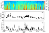 |
Fig. 1 Precipitating solar wind protons and hydrogen ENAs at Mars during December 2021, shown for each MAVEN and Tianwen-1 orbit. (a) Energy spectrum of precipitating solar wind protons. (b) Hydrogen ENA velocity. (c) Hydrogen ENA flux. |
2 Data and methods
2.1 Precipitating solar wind proton observations
Precipitating solar wind protons can interact with the Martian atmosphere and drive sputtering escape. To quantify this process, information on the precipitating proton flux is required. Ideally, this flux should be evaluated near the Martian exobase, where the transition from collisionless to collisional behavior occurs and sputtering becomes effective. This region is often taken to lie near 200 km (e.g., Fu et al. 2020). However, ion-neutral collisions can still occur above this altitude. Chaufray et al. (2007) reported that the charge-exchange probability can reach nearly 50% above 200 km. Consequently, if measurements are restricted to the exobase, the total particle energy ultimately deposited into the atmosphere may be underestimated, because a fraction of the incident energy has already been lost through neutralization and thermalization. For these reasons, many studies adopt an upper altitude limit of ~350 km. For example, Leblanc et al. (2015) assumed that ions with downward velocity vectors lying within a 75° cone around the radial direction would ultimately impact the atmosphere.
In this study, we instead sampled a higher-altitude range of 450–550 km. To ensure that the selected particles can still reach the atmosphere, we adopted a more stringent angular criterion and restricted the allowable angle to 60°. Two instruments – the Solar Wind Ion Analyzer (SWIA; Halekas et al. 2015) and the SupraThermal and Thermal Ion Composition instrument (STATIC; McFadden et al. 2015) – on board MAVEN are capable of measuring the precipitating proton flux. For SWIA, the 3D measurements comprise 64 angular bins. We classified an anode as observing precipitating ions when, within 450–550 km, the angle between the center of the anode field of view (FOV) and the local zenith direction is smaller than 60°. We then selected all anodes satisfying this criterion throughout the altitude interval and summed their counts to obtain the precipitating flux. To ensure adequate spatial coverage, we retained only the intervals in which the FOV coverage, defined as the sum of the solid angles of the selected SWIA bins divided by the solid angle of a cone with a 60° apex angle, 2π(1 – cos60°) ≈ 3.14 sr, exceeds 65%. For each time and energy bin, we summed the counts from all selected anodes to compute the precipitating flux. Due to its limited FOV, STATIC was not used for flux calculations. Figure 1a presents the energy spectrum of the precipitating protons as a function of date, clearly showing that the proton flux exhibits pronounced temporal variability.
2.2 Hydrogen ENA observations
Tianwen-1, China’s first Mars exploration mission, was launched on July 23, 2020, and began its orbital science observations in November 2021. Hydrogen ENA observations used in this study were obtained from the Mars Ion and Neutral Particle Analyzer (MINPA; Kong et al. 2020) on board the Tianwen-1 orbiter. For the MINPA ENA detection, the ambient neutral atoms were ionized upon impact at an Al2O3 conversion surface and subsequently analyzed by an electrostatic analyzer (ESA) and time-of-flight (TOF) system. This design enables ENA measurements over an energy range from 57 eV to 3.5 keV with an energy resolution of approximately 68%, and MINPA is capable of resolving energetic neutral hydrogen, helium, and oxygen.
The instrument’s FOV is 360° × 9.7°. Advanced by the orbiter attitude and the MINPA mounting position, this FOV can cover the Sun-pointing direction. In this study, we focused on the hydrogen ENA measurements. By leveraging the advanced Extreme Ultraviolet (EUV) absorption technique (Wang et al. 2023), MINPA can detect ENAs directly from the Sun-pointing direction, enabling direct observations of penetrating hydrogen ENAs (Ma et al. 2025). For our analysis, we used the dataset from December 2021, when Tianwen-1 spent a substantial fraction of its orbit upstream of the Martian bow shock, providing favorable conditions for upstream solar wind hydrogen ENA observations. Due to the low count rates, the original 16 s data of hydrogen ENA fluxes and velocities were averaged over 10 minutes.
The hydrogen ENA count rates measured by MINPA were converted into physical particle fluxes using a dedicated data processing procedure that accounts for the instrument response and calibration characteristics. The performance of the MINPA hydrogen ENA detection unit, including the energy response, angular scattering at the conversion surface, and geometric factors, was characterized through extensive ground calibrations conducted at the MEsskammer fu¨r FlugzeitInStrumente und Time-Of-Flight (MEFISTO) facility at the University of Bern. Based on these calibration results and in-flight measurements, the conversion from count rates to hydrogen ENA fluxes was performed using a parameterized spectral fitting approach. The observed hydrogen ENA count rate spectra in individual viewing sectors were fitted to derive characteristic energies and count-rate amplitudes. The fitted energies were corrected for energy losses at the conversion surface, from which the bulk velocity of hydrogen ENAs was obtained, while the amplitudes were converted into physical fluxes using the corresponding geometric factors. Figures 1b and 1c show the corresponding hydrogen ENA velocities and fluxes during this period, revealing pronounced variability in both parameters.
2.3 Monte Carlo model
To obtain the sputtering escape rates of various atmospheric species, information on the sputtering yield is required, which is defined as the average number of escaping atmospheric molecules produced per incident high energetic particle (Johnson 1994). Given the stochastic nature of particle collisions and the involvement of multiple recoils, sputtering yields are most reliably evaluated with Monte Carlo simulations. This approach has been widely applied in studies of sputter-induced escape on solar system bodies (e.g., Shematovich et al. 2003; Leblanc et al. 2018; Snowden & Higgins 2021; Huang et al. 2024; Curry et al. 2025) and more recently extended to exoplanets (Gu et al. 2023a). In this study, we employed the test particle Monte Carlo model previously developed for the same planet (Ma et al. 2025), which is briefly summarized here for clarity.
The background atmosphere, consisting of CO2, CO, N2, and O, was adopted from Gu et al. (2025) over the altitude range 100–500 km and was assumed to be spherically symmetric. Below 100 km, the mean free path is sufficiently short that particles rapidly lose energy and thermalize to the local temperature within a distance not exceeding 10 m, consistent with local thermalization. At 500 km, the collision probability drops to ~1%, therefore, the atmosphere above this altitude is not expected to exert an appreciable influence on the derived sputtering yields. The Martian background atmosphere is discretized into 80 vertical layers, each with a depth of 5 km.
For a proton or hydrogen ENA entering the Martian upper atmosphere with a specified incident energy and incidence angle, we followed its trajectory step by step under Martian gravity until a collision occurred. Collisions with ambient atmospheric particles were implemented using three independent random numbers uniformly distributed between 0 and 1. The first (R1) was used to sample the altitude of the next collision, z′, according to
 (1)
(1)
where z is altitude, z0 is the initial location, β is the angle between the particle’s velocity vector and the local vertical (downward) direction, and σi and ni are the total collision cross section and number density of species i (CO2, CO, N2, and O), respectively.
Once a collision occurs, a second random number (R2) was generated to select the collision target among CO2, CO, N2, and O. To this end, we defined the selection weight for species i as wi = σiNi∕Σ(σiNi), where σi is the total collision cross section and Ni is the vertical column density of species i between z0 and z′. The incident particle was taken to collide with CO2 if R2 < wCO2, with O if wCO2 ≤ R2 < wCO2 + wO, and with the remaining species by continuing the same cumulative-sum procedure.
After the target species was specified, the scattering angle of the incident particle in the laboratory frame, θLAB, was determined using a third random number (R3):
![Mathematical equation: \theta_{LAB} = [R_3(\theta_{max}^{\alpha_E}-\theta_{min}^{\alpha_E})+\theta_{min}^{\alpha_E}]^{1/\alpha_E}.](/articles/aa/full_html/2026/07/aa60674-26/aa60674-26-eq2.png) (2)
(2)
Here, θmin is the minimum scattering angle (taken to be 0.01 °), and θmax is the maximum scattering angle, given by
 (3)
(3)
where
 (4)
(4)
In Eq. (4), ma and mb are the masses of the incident and target particles, respectively, ε is the kinetic energy of the incident particle, and Q is the kinetic energy converted into internal energy in an inelastic collision. In the present model, ionization, excitation, and dissociation were included only as inelastic energy-loss channels. That is, they reduced the kinetic energy available to the post-collision particles, but the chemical products of these processes were not explicitly followed. For example, when CO2 dissociation occurred, the subsequent CO, O, or C fragments were not tracked as separate particles in the Monte Carlo simulation. The model therefore follows the trajectories and energies of the incident particle and recoiling atmospheric target particles, while treating internal excitation, ionization, and dissociation as energy losses. We computed Q following the formalism of Firsov (1959):
![Mathematical equation: Q(eV) = \frac{4.3\times 10^{-8} v (Z_A+Z_B)^{5/3}}{[1+0.3b(Z_A+Z_B)^{1/3}]^5 },](/articles/aa/full_html/2026/07/aa60674-26/aa60674-26-eq5.png) (5)
(5)
where b is the impact parameter in units of Bohr radius, v is the relative velocity in units of centimeters per second, and ZA and ZB are nuclear charge numbers of the incident and target species, respectively.
The scattering angle in the center-of-mass frame, θCM, is related to θLAB through
![Mathematical equation: \begin{split} \theta_{CM} = \arccos \Bigl[ &-\rho_m + \rho_m\cos^2{(\theta_{LAB})} \\ &+ \cos{(\theta_{LAB})}\sqrt{1-\rho_m^2\sin^2{(\theta_{LAB})}} \Bigr]. \end{split}](/articles/aa/full_html/2026/07/aa60674-26/aa60674-26-eq6.png) (6)
(6)
The post-collision velocities of the two collision partners were determined from conservation of momentum and energy.
The above procedure was repeated until one of the following termination criteria was met: (1) the incident proton reaches the lower boundary, or its kinetic energy falls below the local escape energy through a cascade of collisions, in which case it is no longer tracked; (2) the incident proton reaches the upper boundary, where it is assumed to escape the atmosphere if its kinetic energy exceeds the local escape energy, or elastically reflected downward otherwise. To ensure statistical robustness, each simulation included 100 000 incident protons or hydrogen ENAs. A total of 171 simulations were performed, spanning 11 energy levels for hydrogen ENAs and eight for protons, with nine incidence angles per energy level uniformly sampled from 0° to 80°.
We next describe the cross sections adopted to characterize elastic scattering and charge exchange between energetic particles and ambient neutral species. Elastic scattering cross sections for H colliding with CO2, CO, N2, and O were adopted from Lewkow & Kharchenko (2014). Elastic scattering cross sections for H+-O and H+-N2 were taken from Noël & Prölss (1993), and for H+-CO and H+-CO2, we assumed the same elastic scattering cross sections as for H+-N2. For other collision pairs, elastic scattering cross sections below 10 eV were adopted from Gu et al. (2020) and are were to energies above 10 eV by scaling their relative magnitudes to match the energy dependence reported in Lewkow & Kharchenko (2014). Charge-exchange cross sections for H+ with O and N2 were adopted from Lindsay & Stebbings (2005). Similarly, we assumed that the charge-exchange cross sections for H+-CO and H+-CO2 are identical to those for H+-N2. The scattering angle distribution was parameterized by αE in Eq. (2). This parameter was obtained by fitting laboratoryframe differential scattering cross sections using the reduced coordinates ρ and τ (Noël & Prölss 1993):
 (7)
(7)
 (8)
(8)
 (9)
(9)
where ε is the kinetic energy of the incident particle, θLAB is the scattering angle in the laboratory frame, σ is the total scattering cross section, and dσ/dΩ is the differential scattering cross section per unit solid angle Ω. Specifically, at an incident energy of 1 keV, αE for elastic scattering, αE is generally in the range −1.2 to −1.0, corresponding to strongly forward scattering.
3 Results
3.1 Sputtering yields
Figure 2 displays the sputtering yields of CO2 and O induced by precipitating solar wind protons and hydrogen ENAs as functions of incidence angle and incident velocity (or energy). Here, an incidence angle of 0° corresponds to precipitating particles enter the atmosphere perpendicularly. The figure reveals several interesting features.
First, our calculations yield sputtering yields of 2.8×10⁻⁵−2×10⁻² for CO2 and 8×10⁻⁶−3.7×10⁻³ for O induced by hydrogen ENAs, and 3×10⁻⁶−5×10⁻² for CO2 and 1×10⁻⁶−6.5×10⁻³ for O induced by precipitating solar wind protons. Overall, the sputtering yields induced by precipitating solar wind protons exhibit a broader range than those induced by hydrogen ENAs. This behavior arises from the wider incident energy distribution of solar wind protons relative to hydrogen ENAs. The latter mainly originate from the charge exchange between solar wind protons and hydrogen atoms in the Martian exosphere, and thus their velocities are approximately equal to the solar wind speed, with a typical thermal broadening of about 10 eV. In contrast, precipitating solar wind protons are decelerated while passing through the Martian magnetosheath, resulting in a wider range of energies, 101–104 eV, as illustrated in Fig. 1. Therefore, in the subsequent escape rate calculations, we adopted a representative single energy for hydrogen ENAs, whereas for precipitating solar wind protons, the flux and sputtering yields were integrated over their entire energy range.
Second, both CO2 and O sputtering yields increase with increasing incidence angle and incident velocity (or energy). For example, the CO2 sputtering yield induced by hydrogen ENAs rises from 2.8×10⁻⁵ to 2.3×10⁻⁴ as the incident velocity increases from 280 to 800 km s−1 at a fixed incidence angle of 0° Similarly, at an incident velocity of 540 km s−1, the CO2 sputtering yield increases from 1.3×10⁻⁴ to 1.3×10⁻² as the incidence angle increases from 0° to 80°. This behavior reflects that particles with higher kinetic energies generate more atmospheric recoils during energy degradation (e.g., Johnson et al. 2000; Gu et al. 2019, 2023a). Moreover, oblique incidence angles confine hydrogen ENAs and recoil trajectories to higher altitudes, where the lower atmospheric density enhances the escape probability (Johnson et al. 2000; Huang et al. 2024, 2025).
Third, the sputtering yields of CO2 are generally larger than those of O, with this contrast becoming more pronounced at higher incident velocities (or energies). Specifically, at a fixed incidence angle of 0°, the CO2 and O sputtering yields induced by hydrogen ENAs are 2.8×10⁻⁵ and 8×10⁻⁶, respectively, for an incident velocity of 280 km s−1, while the corresponding values are 2.3×10⁻⁴ and 4.7×10⁻⁵ at 800 km s−1. This behavior can be explained by the altitude-dependent atmospheric composition. At oblique incidence angles and low velocities, hydrogen ENAs and recoil trajectories are confined to higher altitudes where the O/CO2 mixing ratio is relatively high. Conversely, at higher speeds, they penetrate deeper into the atmosphere, where the ratio decreases rapidly above the Martian homopause.
For illustration, Fig. 3a shows the production yields of all ambient particles for hydrogen ENAs with an incident angle of 50° and an incident velocity of 400 km s−1, while Fig. 3b presents the production yields of above-threshold O and CO2 recoils, defined as particles whose nascent kinetic energies exceed the local escape energies of 1.8 and 4.8 eV, respectively. Figure 3c further shows the altitude distribution of the ultimately escaping O and CO2 particles, i.e., particles that retain sufficient kinetic energy after subsequent collisional transport and finally escape through the upper boundary. Figure 3a demonstrates that the production yield decreases rapidly with decreasing altitude as the background gas density increases approximately exponentially, indicating that the maximum penetration depth is below 100 km.
The comparison between Figs. 3b and 3c highlights the important distinction between above-threshold recoil production and actual escape. Although a substantial fraction of abovethreshold O and CO2 recoils is produced below the exobase, these particles do not necessarily escape. Particles generated in dense regions may undergo additional collisions, lose kinetic energy, change direction, and eventually become thermalized before reaching the exobase. As a result, the production yield of ultimately escaping particles shown in Fig. 3c is much smaller than the above-threshold production yield shown in Fig. 3b. The altitude dependence in Fig. 3c indicates that the final escaping population is preferentially associated with higher altitudes, where collisional attenuation is weaker. This result demonstrates that a nascent energy exceeding the local escape energy is only a necessary condition for escape, not a sufficient one. The final escape probability is controlled by both the initial recoil energy and the subsequent collisional history. Thus, the escape rates reported below were not obtained by directly integrating the above-threshold production in Fig. 3b, but by following particles through the full Monte Carlo transport process until they either escaped, thermalized, or were lost through downward transport.
Furthermore, the calculated total production yield is on the order of unity, comparable to the results reported in Lewkow & Kharchenko (2014). Figures 3b and 3c indicate that collisional filtering is strongest at lower altitudes, whereas above roughly 150 km a large fraction of above-threshold recoils can survive subsequent collisions and escape in this particular simulation. Thus, the escape probability increases with altitude as the probability of further collisions decreases, rather than being controlled only by production near the nominal exobase.
Figure 4 shows the nascent energy distributions of O and CO2 recoils in the 1–10 eV range produced at altitudes of 100– 500 km. The distributions are dominated by low-energy recoils, but a weak high-energy tail extends beyond the local CO2 escape energy. Although this tail represents only a small fraction of the recoil population, it is the component most relevant to the production of above-threshold CO2 recoils and to the residual escaping fraction.
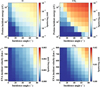 |
Fig. 2 Distributions of the O and CO2 sputtering yields induced by precipitating lar wind protons (upper row) and hydrogen ENAs (bottom row) as functions of incidence angle and incident velocity (or energy). |
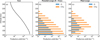 |
Fig. 3 Production and escape yield profiles for hydrogen ENAs with an incident angle of 50° and an incident velocity of 400 km s−1. (a) Total recoil production yield of all ambient particles per incident H ENA per unit altitude. (b) Production yield of above-threshold O and CO2 recoils, defined as particles whose nascent kinetic energies exceed the local escape energy. (c) Production altitude distribution of ultimately escaping O and CO2 particles after subsequent collisional transport. The difference between panels b and c illustrates the strong collisional filtering of hot recoils produced in dense atmospheric regions. |
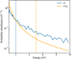 |
Fig. 4 Energy distributions of nascent O and CO2 recoils in the 1–10 eV range. The vertical dashed lines indicate the corresponding escape energies. |
3.2 Comparison with Lewkow and Kharchenko (2014)
It is useful to compare our results with those of Lewkow & Kharchenko (2014), who performed Monte Carlo simulations of atmospheric sputtering on Mars induced by precipitating hydrogen ENAs. They concluded that heavy species such as CO2 and Ar have no realistic probability of escape, whereas our calculations reveal a nonzero CO2 sputtering yield under the precipitating proton and hydrogen ENA conditions considered here. This apparent difference is important because it concerns whether light incident particles can contribute to the escape of heavy neutral species from Mars.
A key point in this comparison is the distinction between above-threshold recoil production and actual escape. In a collision cascade, some CO2 recoils may be produced with nascent kinetic energies exceeding the local escape energy. However, this condition alone does not guarantee escape. If these particles are produced deep in the atmosphere, they may undergo subsequent collisions, lose kinetic energy, change direction, and become thermalized before reaching the exobase. Therefore, the production of above-threshold CO2 recoils should not be interpreted as the CO2 sputtering yield.
Our Monte Carlo calculation follows each energetic incident particle and recoil through its subsequent collisional history until it reaches the lower boundary, becomes energetically unable to escape, or crosses the upper boundary with kinetic energy exceeding the local escape energy. The CO2 sputtering yield reported here therefore represents only the subset of recoils that survive this collisional transport process. This distinction is illustrated directly in Fig. 3. Figure 3b shows the production of above-threshold O and CO2 recoils, whereas Fig. 3c shows the much smaller subset that ultimately escapes. The large reduction from Figs. 3b to 3c demonstrates that most hot recoils, especially those produced at low altitudes, are removed by subsequent collisions and thermalization before they can escape. This behavior is consistent with the physical argument of Lewkow & Kharchenko (2014) that heavy recoils generated deep in the atmosphere have a very low escape probability.
The main difference between the two calculations appears to arise before collisional transport, namely in the nascent CO2 recoil energy distribution. In Lewkow & Kharchenko (2014), the production of nascent CO2 molecules with energies exceeding the escape energy is essentially negligible. By contrast, our Monte Carlo treatment produces a small but finite high-energy tail. Figure 4 supports this interpretation by showing that the nascent CO2 recoil distribution is dominated by low-energy particles, while a weak high-energy tail extends beyond the local CO2 escape energy. Although this tail represents only a small fraction of the total nascent CO2 population, it is the component relevant to the above-threshold recoil production and to the final escaping fraction after collisional attenuation.
This difference is likely related to the adopted angular distribution of the differential scattering cross section. Rare large-angle scattering events can transfer substantially more kinetic energy to CO2 than the mean collision, and the probability assigned to this angular tail can therefore strongly affect the production of above-threshold CO2 recoils. Figure 5 compares the differential cross sections for 1 keV H–CO2 collisions in the center-of-mass frame. The distribution from Lewkow & Kharchenko (2014) was calculated using their analytical formula, whereas the distribution used in the present study was estimated from 1 000 000 randomly sampled scattering events using Eq. (2), with a characteristic value of αE = −0.85. Although the two distributions are broadly similar over most scattering angles, the sampled distribution gives a slightly larger probability at large scattering angles. This small difference is important for heavy-species escape because the escaping CO2 population is controlled by rare, high-energy recoil events rather than by the mean energy transfer.
Several model differences may also contribute to the quantitative discrepancy. The present study uses precipitating solar wind proton fluxes derived from MAVEN/SWIA and hydrogen ENA fluxes derived from Tianwen-1/MINPA, whereas Lewkow & Kharchenko (2014) adopted prescribed incident hydrogen ENA conditions. Differences in the background atmosphere, incident energy distribution, angular distribution, and collision treatment may also affect the altitude distribution and energy spectrum of nascent recoils. However, because CO2 escape is controlled by the small high-energy tail of the recoil distribution, the treatment of energy transfer during individual collisions, especially the angular distribution of the differential cross section, is likely a particularly important factor.
Finally, we emphasize that our results should be viewed as complementary to, rather than in direct contradiction with, Lewkow & Kharchenko (2014). Both studies indicate that hydrogen ENA/proton-induced escape of heavy species is strongly limited by collisional thermalization. The main difference lies in the rare high-energy tail of the nascent CO2 recoil distribution: in our calculation, a small fraction of CO2 recoils can acquire energies above the local escape threshold and, after subsequent collisional filtering, survive to escape under the observationally constrained precipitating particle conditions examined here. Accordingly, the CO2 sputtering yield reported in this work should be regarded as the final escaping component of this rare high-energy recoil population after thermalization and collisional attenuation, rather than as the total production of energetic or above-threshold CO2 recoils.
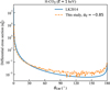 |
Fig. 5 Comparison of differential cross sections for 1 keV H–CO2 collisions in center-of-mass frame. The values indicated by the solid blue line were derived from the analytical formula of Lewkow & Kharchenko (2014), while the values indicated by the dashed orange line were estimated from 1 000 000 randomly sampled scattering events using Eq. (2), with a characteristic value of αE = −0.85. |
3.3 Sputtering-induced escape fluxes
By combining the calculated sputtering yields of CO2 and O with observations of precipitating solar wind protons and hydrogen ENAs, we can estimate the corresponding escape rates driven by atmospheric sputtering. For a given species i, its hemispheric escape rate Lij induced by energetic particles j is given by
 (10)
(10)
where RMars = 3400 km is the solid body radius of Mars, zupper = 500 km is upper boundary, θ is the incidence angle, Yij is the sputtering yields of species i induced by j, and Φ j is the incident flux of j.
Figure 6 presents the CO2 and O escape rates induced by precipitating solar wind protons (panel a) and hydrogen ENAs (panel b) during December 2021. According to our calculations, the median CO2 and O escape rates are 1×10²² s−1 and 1×10²¹ s−1 for precipitating solar wind protons, and 1.4×10²² s−1 and 8× 10²¹ s−1 for hydrogen ENAs. The figure clearly shows that for hydrogen ENAs, the sputter-induced escape rate of CO2 generally exceeds that of O, whereas for precipitating solar wind protons, the escape rates of the two species are comparable. However, during intervals of strong precipitating proton flux at low energies, the O escape rate becomes comparable in magnitude to that of CO2. Specifically, on December 3, when the low-energy precipitating proton flux is significantly enhanced, the daily averaged CO2 and O escape rates driven by precipitating proton sputtering are 3×10²² s−1 and 7×10²¹ s−1, respectively. This trend is consistent with the fact that precipitating solar wind protons possess higher average incident energies than hydrogen ENAs.
It is also necessary to compare the relative importance of these two sputtering sources. This comparison is shown in Figs. 6c and 6d, which present the daily averaged CO2 and O escape rates induced by the two sources described above. The figures show that precipitating solar wind protons generally produce stronger CO2 escape, whereas hydrogen ENAs drive stronger O escape. However, hydrogen ENAs can produce comparable or even greater escape rates during periods of abnormally enhanced ENA flux, as indicated by the spike-like features in Fig. 1c on December 9, 16, and 17.
The sputter-induced escape rates derived here were compared with those reported in previous studies. Specifically, using a precipitating hydrogen ENA flux of 9.2×107 cm−2 s−1, which is one order of magnitude larger than the incident flux considered in this study, Lewkow & Kharchenko (2014) obtained an O escape rate of ~8×10²² s−1. More recently, Shematovich (2017) estimated an O escape rate of 8×10²³ s−1 to 4.5×1024 s−1 for comparable hydrogen ENA precipitation conditions. Using a modeled spectrum of precipitating solar-wind protons (Shematovich 2017), which is larger than the SWIA-based spectrum adopted here, that study also reported an O escape rate of 1.1×10²³ s−1 driven by precipitating solar-wind protons. Given that we adopted a substantially smaller hydrogen ENA and proton flux, these published estimates are broadly consistent with our results for O loss. Interestingly, previous studies have largely focused on sputtering-driven O loss and did not explicitly quantify CO2 escape, whereas our calculations indicate that CO2 escape is generally stronger than O under the same precipitation conditions.
4 Discussion and concluding remarks
This study quantifies atmospheric sputtering on Mars driven by hydrogen ENAs and precipitating solar wind protons, using Monte Carlo simulations constrained by Tianwen-1 and MAVEN observations. Both particle populations contribute to the nonthermal escape of CO2 and O, though their relative importance depends strongly on the incident energy spectrum and geometry. The calculated sputtering yields of CO2 and O increase with both incidence angle and incident velocity (or energy), consistent with enhanced recoil production and greater escape probabilities in the rarefied upper atmosphere. Precipitating solar wind protons, characterized by a broader and higher-energy spectrum, generally produce stronger CO2 and O escape, whereas hydrogen ENAs can generate comparable or even higher escape rates during episodes of abnormally enhanced ENA fluxes. This highlights the dynamic coupling between solar wind variability and atmospheric erosion efficiency.
The sputtering source examined here should be distinguished from sputtering driven by pickup O+ ions, which has been the focus of many previous studies. Because of their larger mass and, in many cases, higher characteristic energies, pickup O+ ions can transfer momentum to atmospheric species more efficiently and are therefore expected to be more effective at ejecting heavy neutrals such as CO2 and Ar. By contrast, the present study focused specifically on precipitating solar wind protons and hydrogen ENAs. These particles are lighter and less efficient per incident particle, but their precipitation is directly linked to the variable solar wind interaction with Mars and can therefore provide a complementary, condition-dependent sputtering source. Accordingly, the escape rates reported here should not be interpreted as a complete estimate of all sputtering escape at Mars, but rather as an observationally constrained estimate of the proton/hydrogen ENA-induced component.
Our results also show that heavy-species escape by pro-ton/hydrogen ENA-induced sputtering is strongly regulated by collisional thermalization. Although CO2 recoils with nascent energies exceeding the local escape energy can be produced, only a small fraction ultimately survive subsequent collisions and escape. This distinction is important when comparing with Lewkow & Kharchenko (2014), who emphasized that heavy species such as CO2 and Ar have very low escape probabilities under hydrogen ENA precipitation. Our calculations are consistent with the general physical picture that heavy recoils produced deep in the atmosphere are efficiently thermalized. The nonzero CO2 escape rates obtained here represent the residual escaping fraction after strong collisional filtering, rather than the total production rate of energetic or above-threshold CO2 recoils.
Our calculations suggest equivalent total O and C escape rates of 1022–1023 s−1, driven by hydrogen ENA and precipitating solar wind proton sputtering. For comparison, photochemical escape, primarily through dissociative recombination of O2+, is the dominant present-day source of atomic oxygen loss on Mars, yielding escape rates on the order of 1025–1026 s−1 (e.g., Fox & Hac´ 2009, 2014, 2018; Cravens et al. 2017; Lillis et al. 2017). Photochemical escape of carbon, produced mainly by photolysis of CO2 and CO, contributes a total C escape rate of approximately 1023–1024 s−1 (e.g., Fox & Bakalian 2001; Cui et al. 2019; Lo et al. 2021; Gu et al. 2023b; Ramstad et al. 2015). Ion pickup and ion outflow processes, which transport charged species along open magnetic field lines, provide additional losses of 1023– 1025 s−1 for O+ or O2+ and 1022–1024 s−1 for CO2+ (e.g., Barabash et al. 2007; Nilsson et al. 2010; Maes et al. 2021; Li et al. 2023; Song et al. 2025). Although the sputtering escape rates for O inferred in this study and previous work (e.g., Lewkow & Kharchenko 2014; Leblanc et al. 2018; Ma et al. 2025) are generally smaller, typically on the order of 1022–1023 s−1 under moderate solar activity, this process may at times dominate the escape of C on Mars by driving CO2 loss. Moreover, sputtering remains uniquely important because it can eject heavy neutral species, particularly Ar (e.g., Curry et al. 2025), that are largely inaccessible to photochemical or ion processes. Over geological timescales, this mechanism may have contributed a substantial fraction of the ancient Martian atmospheric loss.
Overall, our results indicate that precipitating solar wind protons and hydrogen ENAs make comparable contributions to nonthermal escape on Mars. Coordinated Tianwen-1 and MAVEN observations provide an effective means to constrain these mechanisms simultaneously. The present work therefore complements previous studies of pickup-ion sputtering by isolating the contribution from light incident particles, namely proton and hydrogen ENAs, under observationally constrained conditions. Future missions equipped with higher-sensitivity ENA imagers and ion analyzers will be critical for quantifying the variability, efficiency, and cumulative impact of sputtering on Mars’ atmospheric evolution and long-term habitability.
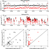 |
Fig. 6 CO2 and O escape rates driven by precipitating solar wind protons and hydrogen ENAs. (a) CO2 and O escape rates driven by precipitating solar wind protons for each MAVEN orbit. (b) CO2 and O escape rates driven by hydrogen ENAs for each Tianwen-1 orbit. (c) Comparison of daily averaged CO2 escape rates driven by precipitating solar wind protons and hydrogen ENAs, with the dashed line indicating equal escape rates. (d) Same as panel (c) but for O escape. |
Acknowledgements
The authors acknowledge supports from the National Natural Science Foundation of China through grants 42241112, 42522803 and 42475134.
References
- Barabash, S., Fedorov, A., Lundin, R., & Sauvaud, J.-A. 2007, Science, 315, 501 [CrossRef] [Google Scholar]
- Brain, D., Barabash, S., Boesswetter, A., et al. 2010, Icarus, 206, 139 [Google Scholar]
- Chaufray, J. Y., Modolo, R., Leblanc, F., et al. 2007, J. Geophys. Res. Planets, 112, E09009 [Google Scholar]
- Cravens, T. E., Rahmati, A., Fox, J. L., et al. 2017, J. Geophys. Res. Space Phys., 122, 1102 [Google Scholar]
- Cui, J., Wu, X.-S., Gu, H., Jiang, F.-Y., & Wei, Y. 2019, A&A, 621, A23 [NASA ADS] [CrossRef] [EDP Sciences] [Google Scholar]
- Curry, S. M., Hara, T., Luhmann, J. G., et al. 2025, Sci. Adv., 11, eadt1538 [Google Scholar]
- Dubinin, E., Winningham, D., Fränz, M., et al. 2006, Icarus, 182, 343 [Google Scholar]
- Fang, X., Bougher, S. W., Johnson, R. E., et al. 2013, Geophys. Res. Lett., 40, 1922 [NASA ADS] [CrossRef] [Google Scholar]
- Firsov, O. B. 1959, Sov. J. Exp. Theor. Phys., 9, 1076 [Google Scholar]
- Fox, J. L., & Bakalian, F. M. 2001, J. Geophys. Res., 106, 28785 [NASA ADS] [CrossRef] [Google Scholar]
- Fox, J. L., & Hac´, A. B. 2009, Icarus, 204, 527 [NASA ADS] [CrossRef] [Google Scholar]
- Fox, J. L., & Hac´, A. B. 2014, Icarus, 228, 375 [NASA ADS] [CrossRef] [Google Scholar]
- Fox, J. L., & Hac´, A. B. 2018, Icarus, 300, 411 [NASA ADS] [CrossRef] [Google Scholar]
- Fu, M., Cui, J., Wu, X., Wu, Z., & Li, J. 2020, Earth Planet. Phys., 4, 4 [Google Scholar]
- Gu, H., Cui, J., Niu, D.-D., et al. 2019, A&A, 623, A18 [NASA ADS] [CrossRef] [EDP Sciences] [Google Scholar]
- Gu, H., Cui, J., Niu, D., He, Z., &Li, K. 2020, ApJ, 902, 121 [Google Scholar]
- Gu, H., Wu, X., Cui, J., et al. 2025, AJ, 169, 74 [Google Scholar]
- Gu, H., Wu, X., Huang, X., Guo, J., & Cui, J. 2023a, ApJ, 959, 80 [Google Scholar]
- Gu, H., Wu, X.-S., & Cui, J. 2023b, A&A, 672, A177 [NASA ADS] [CrossRef] [EDP Sciences] [Google Scholar]
- Halekas, J. S., Taylor, E. R., Dalton, G., et al. 2015, Space Sci. Rev., 195, 125 [CrossRef] [Google Scholar]
- Huang, X., Gu, H., Ni, Y., Zhao, J., & Cui, J. 2024, J. Geophys. Res. Planets, 129, e2023JE008129 [Google Scholar]
- Huang, X., Gu, H., & Cui, J. 2025, A&A, 702, A5 [NASA ADS] [CrossRef] [EDP Sciences] [Google Scholar]
- Jakosky, B. M. 2021, Ann. Rev. Earth Planet. Sci., 49 [Google Scholar]
- Jakosky, B. M., Lin, R. P., Grebowsky, J. M., et al. 2015, Space Sci. Rev., 195, 3 [CrossRef] [Google Scholar]
- Jakosky, B. M., Slipski, M., Benna, M., et al. 2017, Science, 355, 1408 [CrossRef] [Google Scholar]
- Jakosky, B. M., Brain, D., Chaffin, M., et al. 2018, Icarus, 315, 146 [NASA ADS] [CrossRef] [Google Scholar]
- Johnson, R. E. 1994, Space Sci. Rev., 69, 215 [Google Scholar]
- Johnson, R. E., Schnellenberger, D., & Wong, M. C. 2000, J. Geophys. Res., 105, 1659 [Google Scholar]
- Kite, E. S. 2019, Space Sci. Rev., 215, 10 [Google Scholar]
- Kong, L., Zhang, A., Tian, Z., et al. 2020, Earth Planet. Phys., 4, 333 [Google Scholar]
- Lammer, H., Chassefière, E., Karatekin, Ö., et al. 2013, Space Sci. Rev., 174, 113 [NASA ADS] [CrossRef] [Google Scholar]
- Leblanc, F., Modolo, R., Curry, S., et al. 2015, Geophys. Res. Lett., 42, 9135 [Google Scholar]
- Leblanc, F., Martinez, A., Chaufray, J. Y., et al. 2018, Geophys. Res. Lett., 45, 4685 [NASA ADS] [CrossRef] [Google Scholar]
- Lewkow, N. R., & Kharchenko, V. 2014, ApJ, 790, 98 [Google Scholar]
- Li, G., Lu, H., Li, Y., et al. 2023, ApJ, 957, 92 [Google Scholar]
- Lillis, R. J., Deighan, J., Fox, J. L., et al. 2017, J. Geophys. Res. Space Phys., 122, 3815 [NASA ADS] [CrossRef] [Google Scholar]
- Lindsay, B. G., & Stebbings, R. F. 2005, J. Geophys. Res. Space Phys., 110, A12213 [Google Scholar]
- Lo, D. Y., Yelle, R. V., Lillis, R. J., & Deighan, J. I. 2021, Icarus, 360, 114371 [NASA ADS] [CrossRef] [Google Scholar]
- Luhmann, J. G., Johnson, R. E., & Zhang, M. H. G. 1992, Geophys. Res. Lett., 19, 2151 [Google Scholar]
- Ma, J., Kong, L., Gu, H., et al. 2025, Earth Planet. Phys., 9, 1147 [Google Scholar]
- Maes, L., Fraenz, M., McFadden, J. P., & Benna, M. 2021, J. Geophys. Res. Space Phys., 126, e28608 [Google Scholar]
- McFadden, J. P., Kortmann, O., Curtis, D., et al. 2015, Space Sci. Rev., 195, 199 [CrossRef] [Google Scholar]
- Nilsson, H., Carlsson, E., Brain, D. A., et al. 2010, Icarus, 206, 40 [Google Scholar]
- Noël, S., & Prölss, G. W. 1993, J. Geophys. Res., 98, 17317 [Google Scholar]
- Ramirez, R. M., & Craddock, R. A. 2018, Nat. Geosci., 11, 230 [Google Scholar]
- Ramstad, R., Barabash, S., Futaana, Y., et al. 2015, J. Geophys. Res. Planets, 120, 1298 [Google Scholar]
- Shematovich, V. I. 2017, Sol. Syst. Res., 51, 249 [Google Scholar]
- Shematovich, V. I. 2021, Sol. Syst. Res., 55, 324 [Google Scholar]
- Shematovich, V. I., Johnson, R. E., Michael, M., & Luhmann, J. G. 2003, J. Geophys. Res. Planets, 108, 5087 [Google Scholar]
- Snowden, D., & Higgins, A. 2021, Icarus, 354, 113929 [Google Scholar]
- Song, Y., Lu, H., Cao, J., et al. 2025, ApJ, 984, 129 [Google Scholar]
- Wang, Y.-C., Luhmann, J. G., Leblanc, F., et al. 2014, J. Geophys. Res. Planets, 119, 93 [Google Scholar]
- Wang, Y.-C., Luhmann, J. G., Fang, X., et al. 2015, J. Geophys. Res. Planets, 120, 34 [Google Scholar]
- Wang, X. D., Alho, M., Jarvinen, R., et al. 2018, J. Geophys. Res. Space Phys., 123, 8730 [Google Scholar]
- Wang, L., Li, L., Li, W., et al. 2023, Atmosphere, 15, 19 [Google Scholar]
- Wordsworth, R. D. 2016, Ann. Rev. Earth Planet. Sci., 44, 381 [Google Scholar]
- Zou, Y., Zhu, Y., Bai, Y., et al. 2021, Adv. Space Res., 67, 812 [Google Scholar]
All Figures
|
Fig. 1 Precipitating solar wind protons and hydrogen ENAs at Mars during December 2021, shown for each MAVEN and Tianwen-1 orbit. (a) Energy spectrum of precipitating solar wind protons. (b) Hydrogen ENA velocity. (c) Hydrogen ENA flux. |
| In the text | |
|
Fig. 2 Distributions of the O and CO2 sputtering yields induced by precipitating lar wind protons (upper row) and hydrogen ENAs (bottom row) as functions of incidence angle and incident velocity (or energy). |
| In the text | |
|
Fig. 3 Production and escape yield profiles for hydrogen ENAs with an incident angle of 50° and an incident velocity of 400 km s−1. (a) Total recoil production yield of all ambient particles per incident H ENA per unit altitude. (b) Production yield of above-threshold O and CO2 recoils, defined as particles whose nascent kinetic energies exceed the local escape energy. (c) Production altitude distribution of ultimately escaping O and CO2 particles after subsequent collisional transport. The difference between panels b and c illustrates the strong collisional filtering of hot recoils produced in dense atmospheric regions. |
| In the text | |
|
Fig. 4 Energy distributions of nascent O and CO2 recoils in the 1–10 eV range. The vertical dashed lines indicate the corresponding escape energies. |
| In the text | |
|
Fig. 5 Comparison of differential cross sections for 1 keV H–CO2 collisions in center-of-mass frame. The values indicated by the solid blue line were derived from the analytical formula of Lewkow & Kharchenko (2014), while the values indicated by the dashed orange line were estimated from 1 000 000 randomly sampled scattering events using Eq. (2), with a characteristic value of αE = −0.85. |
| In the text | |
|
Fig. 6 CO2 and O escape rates driven by precipitating solar wind protons and hydrogen ENAs. (a) CO2 and O escape rates driven by precipitating solar wind protons for each MAVEN orbit. (b) CO2 and O escape rates driven by hydrogen ENAs for each Tianwen-1 orbit. (c) Comparison of daily averaged CO2 escape rates driven by precipitating solar wind protons and hydrogen ENAs, with the dashed line indicating equal escape rates. (d) Same as panel (c) but for O escape. |
| In the text | |
Current usage metrics show cumulative count of Article Views (full-text article views including HTML views, PDF and ePub downloads, according to the available data) and Abstracts Views on Vision4Press platform.
Data correspond to usage on the plateform after 2015. The current usage metrics is available 48-96 hours after online publication and is updated daily on week days.
Initial download of the metrics may take a while.