


| Issue |
A&A
Volume 710, June 2026
|
|
|---|---|---|
| Article Number | A182 | |
| Number of page(s) | 27 | |
| Section | Planets, planetary systems, and small bodies | |
| DOI | https://doi.org/10.1051/0004-6361/202659499 | |
| Published online | 11 June 2026 | |
Scattering and sputtering on the lunar surface
Insights from negative ions observed at the surface
1
Swedish Institute of Space Physics (IRF),
Bengt Hultqvists väg 1,
Kiruna
98192,
Sweden
2
Department of Physics, Umeå University,
907 36
Umeå,
Sweden
3
National Space Science Center (NSSC), Chinese Academy of Sciences (CAS),
No. 1 Nanertiao, Zhongguancun, Haidian district,
Beijing,
100190,
China
4
University of Chinese Academy of Sciences,
No. 1 Yanqihu East Road, Huairou district,
Beijing
101408,
China
★ Corresponding author: This email address is being protected from spambots. You need JavaScript enabled to view it.
Received:
18
February
2026
Accepted:
14
April
2026
Abstract
Context. Airless planetary bodies are directly exposed to solar wind ions, which can scatter or become implanted upon impact with the regolith-covered surface, while also sputtering surface atoms.
Aims. We constructed a semi-analytical model for the scattering of ions of hundreds of electron volts (eV) and the sputtering of surface atoms, both resulting in the emission of negative ions from the lunar surface. Our model contains a novel description of the scattering process that is physics-based and constrained by observations.
Methods. We used data from the Negative Ions at the Lunar Surface (NILS) instrument on the Chang’e-6 lander to update prior knowledge of ion scattering and sputtering from lunar regolith through Bayesian inference.
Results. Our model shows a good agreement with the NILS data. We find that a precipitating solar wind proton has a roughly 22−6.1+4.9 % chance of scattering from the lunar surface in any charge state and 8.1−3.9+7.9 % chance of sputtering a surface hydrogen atom. The resulting ratio of scattered to sputtered hydrogen flux is ηsc/ηsp = 1.5−1.1+1.5 for a proton speed of 300 km/s. We found a high probability (7-20%) that a hydrogen atom leaves the surface negatively charged. The angular emission distributions at near-grazing angles for both scattered and sputtered fluxes are controlled by surface roughness. Our model also indicates significant inelastic energy losses for hydrogen interacting with the regolith, suggesting a longer effective path length than previously assumed. Finally, we estimated a surface binding energy of 5.5 eV, consistent with the observations.
Conclusions. Our model describes the scattering and sputtering of particles of any charge state from any homogeneous, multi-species surface. Using NILS data, we successfully applied the model to update our understanding of solar wind interacting with lunar regolith and the emission of negative hydrogen ions.
Key words: atomic processes / methods: data analysis / methods: statistical / space vehicles: instruments / Moon
© The Authors 2026
 Open Access article, published by EDP Sciences, under the terms of the Creative Commons Attribution License (https://creativecommons.org/licenses/by/4.0), which permits unrestricted use, distribution, and reproduction in any medium, provided the original work is properly cited.
This article is published in open access under the Subscribe to Open model. This email address is being protected from spambots. You need JavaScript enabled to view it. to support open access publication.
1 Introduction
Planetary bodies without atmospheres are directly exposed to the space environment. Continuous space weathering (Pieters & Noble 2016) alters their surfaces and produces a porous, unconsolidated, and fragmented layer of debris known as regolith (Papike et al. 1982; Clark et al. 2002). The regolith acts as the primary interface between airless bodies and the surrounding space environment, controlling how the solar wind and other energetic particles interact with their surfaces. Understanding these interactions is essential for studying surface evolution, elemental composition, and the formation of surface-bounded exospheres.
When a particle interacts with a solid surface, it might be directly reflected by surface atoms or penetrate the solid. Within the solid, the particle can scatter off atoms, lose energy, and eventually exit the material. Alternatively, it may come to rest and be implanted. The reflection of incoming particles is referred to as (back-)scattering. As the particle moves through the material, it transfers energy to atoms of the solid. Some of these energised atoms may be ejected from the surface in a process known as sputtering.
The charge state of particles interacting with a surface is not conserved. Precipitating ions are neutralised when approaching the surface and their original charge state is effectively lost (for example, Jans et al. 2001). Near the surface, particles remain in a (quasi-)neutral charge-state equilibrium that is established on timescales that are much shorter than the total interaction time with the material (Lienemann et al. 2011). As particles leave the surface, their charge states are further modified through chargeexchange processes, eventually reaching a final charge state at distances of several nanometres from the solid. The probability for an emitted particle to reach a particular charge state depends on the energy and species of the particle, but also on surface properties like average composition, adsorbents, atomic structure (crystalline or amorphous), structure defects, or composition impurities (for example, Kawano & Page 1983; Maazouz et al. 1998; Wucher 2008; Wucher et al. 2013; Cartry et al. 2017).
The processes of scattering, sputtering, and charge-exchange have been extensively studied for a wide range of particle-surface combinations. However, because regolith on airless bodies is unique, studies of pristine regolith - as opposed to returned samples, simulants, or simulations - are limited to in situ or space-borne observations.
Among airless bodies, the Moon provides the most accessible example of natural regolith exposed directly to the solar wind and much of our empirical understanding is derived from orbital measurements. The lunar surface is entirely covered by regolith composed primarily of silicate minerals and glassy agglutinates formed by impact melting (Heiken 1975). Most solar wind protons impacting the lunar regolith are absorbed, sourcing the surface with hydrogen and hydroxyl-bearing molecules (Tucker et al. 2019). Approximately 10-20% of incident protons result in the emission of neutral hydrogen with energies greater than 10 eV (McComas et al. 2009; Wieser et al. 2009; Schaufelberger et al. 2011; Rodríguez et al. 2012; Allegrini et al. 2013; Saul et al. 2013; Vorburger et al. 2014; Zhang et al. 2020). These neutrals are produced either by scattering of the incoming protons or by sputtering of hydrogen from the surface (in both cases) followed by neutralisation of the emitted particle. In addition to neutrals, about 0.1-1% of solar wind protons backscatter from the lunar surface as protons (Saito et al. 2008; Lue et al. 2014, 2018) and about 2.5% as negative hydrogen ions (Wieser et al. 2025). Beyond hydrogen, a wide selection of likely sputtered heavier positive ions has been observed (Tanaka et al. 2009; Yokota et al. 2009), along with other energetic neutral atoms, including backscattered helium and sputtered oxygen (Vorburger et al. 2014).
The angular emission functions and the corresponding energy spectra of emitted particles have been reconstructed for energetic neutral hydrogen (Schaufelberger et al. 2011; Lue et al. 2016) and for protons (Lue et al. 2018), using data from orbiting spacecraft. Although these approaches make it possible to image magnetic anomalies (Wieser et al. 2010; Vorburger et al. 2012), the large observation distance from the surface complicates the study of the actual surface interaction. Indeed, orbital observations average over large surface regions of the Moon, blurring small-scale local variations of the precipitating solar wind flux caused by magnetic anomalies (Halekas et al. 2008). In turn, this hides the detailed structure of the angular and energy distributions of emitted particles.
Observations in space are complemented by laboratory experiments and computer simulations. Because access to pristine lunar regolith is limited, laboratory studies are based on returned samples and regolith simulants (for example, Meyer et al. 2011). In parallel, analytical models and numerical simulations enable studies particle transport and emission processes under controlled conditions (for example, von Toussaint et al. 2017; Szabo et al. 2022; Tucker et al. 2019; Szabo et al. 2023b).
Direct measurements at the lunar surface avoid the material limitations of laboratory studies, along with the difficulties inherent in accurately modelling regolith in numerical simulations and the large spatial averaging in observations from orbiting spacecraft. However, only a few instruments have been deployed to date. The Advanced Small Analyzer for Neutrals (ASAN) instrument (Wieser et al. 2020) measured neutral particles emitted from the lunar surface, with the development of a semi-analytical model to describe the energy distribution of scattered and sputtered neutral hydrogen atoms (Wieser et al. 2024). In June 2024, the Negative Ions at the Lunar Surface (NILS) instrument (Canu-Blot et al. 2025), flown on board of the Chinese Chang’e-6 mission (Zeng et al. 2023), provided data for negative ions and electrons emitted from the lunar surface.
In this study, we used NILS data to develop an analytical model for hydrogen scattering and hydrogen sputtering from lunar regolith, including the probability of emission taking the form of a negative ion. The model separates the energy and angular distributions and is constrained by direct measurements from the lunar surface.
2 Instrumentation
The Negative Ions at the Lunar Surface (NILS) is a small negative ion and electron mass-analyzer (Canu-Blot et al. 2025) that was flown on the Chinese Chang’e-6 mission to the far-side of the moon (Zeng et al. 2023).
NILS measured direction-resolved energy and mass spectra of electrons and ions with energies ranging from 3 eV/q to 3 keV/q. In brief, NILS is a single-pixel instrument and can measure only one energy setting and one viewing direction at a time. A complete measurement cycle, scanning all energy and direction settings and transmitting the data to the spacecraft, takes about 100 s.
The energy range is divided into 48 logarithmically-distributed energy bins. The field of view is an angular slice of 120° × 20°, linearly divided into 16 individual viewing directions with different elevation angles relative to the local horizon (Canu-Blot et al. 2025, Fig. 17). An electron-suppression magnet separates ions from the much more abundant electrons. In ion mode, the instrument has a moderate mass resolution of m/Δm ≈ 2, which allows for the separation of negative hydrogen and oxygen ions. The particle mass is determined from a velocity measurement in a time-of-flight cell combined with the known energy-per-charge selected by the electrostatic analyser.
The NILS science data consist of a time series of 3D energy-direction-mass matrices (Wieser et al. 2025). Each matrix contains the number of particles detected during a single measurement cycle. The matrices consist of 48 energy bins, 16 elevation bins, and 64 mass bins, which together define the energy-per-charge, elevation angle, and time-of-flight of the measured particle.
3 Data
On 1 June 2024 at 22:23 UTC, Chang’e-6 landed on the lunar far-side at 153.98°W, 41.64°S. The landing site is close to the large magnetic anomaly cluster in the South Pole-Aitken basin. NILS was operated during the surface-segment of the Chang’e-6 mission. It recorded particle data from the lunar surface for a total of 302 minutes between 2 June 2024 03:01 UTC and 3 June 2024 03:38 UTC, and successfully detected negative ions on the lunar surface (Wieser et al. 2025).
Figure 1 shows the differential number flux of negative hydrogen ions from the lunar surface for different observation geometries. The size of the vertical bars indicates the range of likely values in the (model-agnostic) estimates of the differential flux. The colour of the bars represents the significance of the observation. For energies below 100 eV, the statistical uncertainty in the separation of hydrogen ions from electrons increases. The lines show the contributions from scattering and sputtering, as derived from the particle-surface interaction model described in the following section. While NILS recorded data, the average solar wind proton energy was Esw = 466 eV (±19.6 eV), with an average proton number density of 8.1 ± 2.2 cm−3. The angular observation geometry is illustrated in Fig. 2. The solar zenith angle (SZA) varied between 52° and 47°, the solar azimuth angle (SAA) varied from 43°E to 28°E and the average azimuthal emission angle was φ = 213°. The various panels in Fig. 1 show data for different intervals of the polar emission angle β.
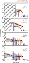 |
Fig. 1 Differential number flux of negative hydrogen ions, J−H, versus emission energy. Vertical bars show flux estimates, with thick and thin bars representing the 68% and 90% highest density intervals, respectively. Bar colour qualitatively reflects signal significance, based on the Widely Applicable Information Criterion (Watanabe 2010) which estimates out-of-sample predictive accuracy, by comparing models with and without hydrogen. Each panel corresponds to a specific emission polar angle interval β (shown in the upper-right inset), where inward arrows indicate the average SZA. The energy-axis arrow marks the average undisturbed solar wind proton energy. Hatched regions indicate energies without data coverage. Lines show the median modelled flux of scattered (black dashed), sputtered (black dash-dotted), and total (solid red) negative hydrogen ions; the gray shading denotes the 68% highest density interval of the total modelled flux. |
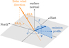 |
Fig. 2 Illustration of the solar wind impinging angles (orange) and emission angles (blue). An arbitrary angular emission profile is drawn, with dashed arrows representing possible emission directions. Both the SZA and the emission polar angle, β, are defined relative to the surface normal. The SAA is relative to the northerly direction, and the emission azimuthal angle, φ, is relative to the SAA. The total scattering angle Ψ is the angle between the solar wind direction and the emission direction. |
4 Interaction model
4.1 A general model
We define the differential number flux J [1/(cm2 sr eV s)] as the flux of emitted particles from a given species, independent of their charge state. We can decompose J into a total flux A [1/(cm2s)] and two normalised functions JE [1/eV] and JΩ [1/sr] that describe the energy and angular distribution of the flux
 (1)
(1)
with ∫JE (E; Ω) dE = 1 and ∫JΩ (Ω) dΩ = 1, where E[eV] is the energy of the emitted particle, and Ω = (β,φ) is the emission solid angle, with β [rad] and φ [rad] the polar and azimuthal emission angles, respectively (see Fig. 2). We factorise the total flux, A, into
 (2)
(2)
with f⊥ [1/(cm2 s)] the incident particle flux normal to the emitting surface. The yield η defines the total number of particles emitted from the surface per incident particle. We can rewrite Eq. (1) in an expanded form,
![Mathematical equation: \mathcal{J} = f_\perp \cdot \mathcal{J}_E \cdot \left[\eta\mathcal{J}_{\Omega}\right],](/articles/aa/full_html/2026/06/aa59499-26/aa59499-26-eq6.png) (3)
(3)
where [ηJΩ] defines the angular yield, that is, the number of particles emitted into a given solid angle per incident particle, integrated over all emission energies.
4.2 Charge states of emitted particles
The quantity J defines the differential flux of all emitted particles of a given species, that is, regardless of their charge state. To obtain the differential flux for a given charge state, q, we introduce the probability of ionisation, Pq, as
 (4)
(4)
where Jq is the differential flux of emitted particles of charge state q. We neglect multiply charged ions, and only consider positive ions (q = +), negative ions (q = –), and neutral particles (q = 0). The probability of ionisation satisfies the following condition
 (5)
(5)
The probability of ionisation depends on the species, energy, emission direction of the emitted particle, and the properties of the surface.
4.3 Independence from the projectile charge state
The definition of J is based on the postulate that the charge state of the projectile does not affect the collision dynamics leading to the eventual emission of a particle(s). In other words, the charge state of f⊥ has no influence. For the scattering of hydrogen and oxygen atoms or ions in the range spanning hundreds to thousands of electron volts (eV), the fraction of negative ions is independent of the initial charge state of the projectile (Lienemann et al. 2011); a charge state equilibrium is achieved almost instantaneously during the interaction process. Auger neutralisation dominates the charge-exchange at long range, whereas resonant charge transfer dominates at close range. The characteristic timescales of these charge-exchange processes are of the order of femtoseconds or less (Wang et al. 2001), while a binary collision occurs hundreds or thousands of times slower (in the case of keV projectiles). Similarly, Schenkel et al. (1997) and Pešić et al. (2007) found that for highly charged ions (q=7-65) with keV energies, the first electron capture typically occurs about 60 a.u. (≈3 nm) above the surface, followed by complete neutralisation within a few tens of femtoseconds.
4.4 Negative ionisation probability
After leaving the surface, a particle continues to exchange electrons with the surface until it reaches its final charge state at distances of several nanometres. The final charge state of particles emitted from a metallic surface is dominantly formed by resonant charge transfer (Los & Geerlings 1990; Gainullin 2020). Charge transfer occurs through electron tunnelling across the potential barrier between the metal conduction band and energetically-overlapping atomic states of the projectile.
The probability of negative ionisation, P−, defined as the probability that a particle reaches a negative charge state after leaving the surface, can be expressed for metallic surfaces as (Eckstein 1981, Eq. (13))
![Mathematical equation: \mathrm{P}^-\left(v_\perp\right) = \exp\left(-v_s/v_\perp\right) \left[1 - \exp\left(-v_f/v_\perp\right)\right],](/articles/aa/full_html/2026/06/aa59499-26/aa59499-26-eq9.png) (6)
(6)
with  as the velocity component of the emitted particle along the surface normal in m/s, m the mass of the particle in kg, E the energy of the particle in J, and (vf, vs) the characteristic velocities associated with the formation and survival of the negative charge state, respectively.
Verbeek et al. (1980) showed that for the emission of hydrogen atoms, the probability of negative ionisation, P−, depends on the emission energy differently than the probability of positive ionisation, P+. While P+ increases with energy, P− reaches a maximum around 2-3 keV and then decreases. Additionally, they found that the probability of negative ionisation increases as the surface work function decreases, consistent with the dominance of resonant charge transfer: a lower work function reduces the energy gap between the conduction band and the electronic states of the projectile, increasing the efficiency of resonant exchange over larger distances. For emitted particles with energies in the hundreds of eV, the probability of negative ionisation can be simplified according to (Wucher 2008, Eqs. (2)-(4)) and expressed as
 (7)
(7)
with vc as the critical velocity of the system and S a constant that controls the probability at high emission velocities (v⊥ ≫ vc). The same relation was found by Lang & Nørskov (1983) when describing the probability of negative ionisation for atoms sputtered off a metal surface.
In contrast to conductive surfaces, the lunar regolith consists of insulating materials with high work functions and large bandgaps. Therefore, the quasi-free electron model used for metal surfaces is not applicable. Nevertheless, Borisov & Esaulov (2000) showed that despite these unfavourable conditions for resonant charge exchange, insulating surfaces can still be efficient producers of negative ions. For example, Wieser et al. (2002) and Wurz et al. (2006) showed that about 3-7% of protons scattering of a MgO surface at grazing incidence are converted to negative hydrogen.
Figure 3 shows measurements of the probability of negative ionisation for 0.5-4 keV hydrogen ions scattering from semiconducting silicon, as reported by Maazouz et al. (1998). The model for metallic surfaces (Eq. (7)) provides a reasonable fit at large v⊥ but underestimates the negative ionisation probability at small v⊥. As in the metallic case, the probability of negative ionisation on semiconductors or insulators depends on the component of the ion velocity perpendicular to the surface. We describe this dependence using a functional form similar to that in Demkov (1963, Eq. (11)), defined as
![Mathematical equation: \mathrm{P}^-(v_\perp) = \mathrm{S} \,\mathrm{sech}^2\left[\mathrm{arcosh}(\sqrt{2}) \left( \dfrac{v_\perp^{50\%}}{v_\perp}\right)^k\right],](/articles/aa/full_html/2026/06/aa59499-26/aa59499-26-eq12.png) (8)
(8)
where the parameter  is the perpendicular speed for which
  is half of its maximum value, that is, S/2; k controls the steepness of the function; S is the ionisation probability for v⊥ → ∞. The values S = 1,
  = 6.4 × 10⁶ m/s and k = 0.26 give a good fit to the data in Fig. 3 over a wide range of v⊥. While S = 1 is not physically valid, the model holds for the range of perpendicular velocities relevant to this study.
The atomic composition of the surface also plays a role: the presence of oxygen atoms is known to increase the probability of positive and, to a lesser extent, negative ionisation (Wucher 2008; Wucher et al. 2013).
 |
Fig. 3 Probability of negative ionisation as a function of the perpendicular emission velocity, v⊥, for 1 keV (≈4.37 × 10⁵ m/s) hydrogen ions scattering off silicon. The mapping to the emission energy for different microscopic emission angles, β′ (Section 4.5) is shown below the figure. Data points (open circles) are taken from Maazouz et al. (1998, Fig. 5a), with the best fit from Eq. (7) shown as a dashed line and that from Eq. (8) shown as a solid line. |
4.5 Emission angles at microscopic scales
The emission angle, β, is defined as the polar angle between the surface normal and the emission direction as shown in Fig. 2. However, the definition of the surface normal depends on the spatial scale considered. When parametrising the angular yield from in-situ data, we use the macroscopic (metre-scale) surface normal (see Sect. 5.2.4) so that our results can be compared with studies based on orbital observations. However, the establishment of the final charge state of an emitted particle is a process that occurs only nanometres above the surface. For that process, the emission angle must therefore be defined with respect to the microscopic surface normal and not the macroscopic average. We denote this microscopic emission angle as β′.
We used the theory of Szabo et al. (2022) to construct a mapping between the macroscopic angle, β, and the microscopic angle, β′. For the lunar regolith, the average microscopic emission angle, β′ [rad], corresponding to a given macroscopic angle, β [rad], is well approximated by the third-order polynomial (a more detailed discussion is provided in Appendix B). This is expressed as
 (9)
(9)
The NILS instrument covers the macroscopic polar angles, β ∊ [45, 90] deg, corresponding to the average microscopic angle, β′ ∊ [49, 72] deg. Due to the high roughness of the lunar regolith, a particle emitted at a grazing angle, (β′ ≳ 70 deg), will likely impact the surface again and is therefore not measured by NILS.
4.6 Putting it all together
We first define the perpendicular influx f⊥ as
 (10)
(10)
where fin [1/(cm2 s)] is the flux of the incident particles and SZA the angle between the incident direction and the surface normal, as schematised in Fig. 2. The actual solar wind incident direction may slightly differ from the Sun direction due to aberration, but we use the term SZA for notational convenience. The formalism naturally applies to any directed incident particle population.
We now assume that an emitted particle is either sputtered from the surface or originates from the scattering of precipitating particles. We express the differential number flux, J, as a sum of the two processes,
 (11)
(11)
where Jsc denotes the scattered flux and Jsp the sputtered flux. Combining Eqs. (3), (4), (10) and (11), we obtain the differential number flux of a specific charge state, q,
![Mathematical equation: \begin{split} \mathcal{J}^q\left(E,\Omega\right) =\, & \mathrm{P}^q f_{\mathrm{in}} \cos\left(\mathrm{SZA}\right)\;\cdot\\ &\big\{\\ &\quad\mathcal{J}_E^\mathrm{sc}\left(E; \Omega\right) \; \left[\eta^\mathrm{sc} \; \mathcal{J}_{\Omega}^\mathrm{sc}\left(\Omega\right)\right]\\ &+\\ &\quad\mathcal{J}_E^\mathrm{sp}\left(E; \Omega\right)\; \left[\eta^\mathrm{sp} \; \mathcal{J}_{\Omega}^\mathrm{sp}\left(\Omega\right)\right] \\ &\big\}, \label{eq:grand_model} \end{split}](/articles/aa/full_html/2026/06/aa59499-26/aa59499-26-eq19.png) (12)
(12)
with ηsc ∊ [0,1] the scattering yield, which naturally cannot exceed one. The sputtering yield can, in principle, exceed one with ηsp ≥ 0. The energy distribution of the scattered and sputtered particles are modelled in the following sections.
4.7 The sputtered component
The energy distribution of atoms sputtered from the lunar surface under solar wind irradiation is described by the analytical model of Ono et al. (2005). Their model extends the earlier formulation of Kenmotsu et al. (2004), which was successfully applied by Wieser et al. (2024) to describe the sputtering of hydrogen atoms from the lunar surface. Unlike the original model by Kenmotsu et al. (2004), the extension accounts for both elastic and inelastic energy losses, the latter being important in the hundreds of eV to few keV range. For projectile energies of hundreds of eV, the extended model shows better agreement with simulations than the earlier model (Ono et al. 2005, Figs. 2 and 3).
Both models are based on the same linear collision cascade (Jamnig 2020, Fig. 2.7) sputtering mechanism described by Kenmotsu et al. (2004). They considered a projectile that penetrates a solid surface, backscatters at a large angle from a surface atom, and loses energy through inelastic and elastic collisions - the latter generating recoil atoms (Sigmund 1969), which are surface atoms displaced from their original lattice position. Recoil atoms with sufficient energy to exit the surface are said to be sputtered. Atoms directly struck by the projectile are referred to as primary recoil atoms, or primary knock-on atoms (PKAs). For light projectiles (e.g. hydrogen, deuterium, helium), secondary, tertiary, and higher order recoil atoms rarely contribute significantly to sputtering, so the models primarily focus on PKAs. Figure 4 illustrates the different stages of the sputtering process as considered in this section.
While the original model by Ono et al. (2005) describes the sputtering of a heavy single-component amorphous material by light ions, we modified it to describe the sputtering of hydrogen by light ions impacting a heavy multi-component amorphous material. We first introduce the notation (P → S) to indicate that a projectile atom P is interacting with an arbitrary surface atom of species S. To emphasise the special case of a projectile atom P interacting with a hydrogen atom in the material, we use the notation (P → H).
We rewrite Eq. (1) from Ono et al. (2005), which describes the energy loss of a projectile as it traverses the surface and the recoiling of hydrogen atoms, to account for the multi-species nature of the interaction,
![Mathematical equation: \begin{split} \overbrace{r_\mathrm{H}\dfrac{\mathrm{d}\sigma_{\left(\mathrm{P}\rightarrow \mathrm{H}\right)}\left(E,E_0\right)}{\mathrm{d}E_0}}^{\left(1\right)}&= \overbrace{\dfrac{\partial F_{\mathrm{PKA}}\left(E,E_0\right)}{\partial E}}^{\left(2\right)} \\ &{\cdot}\!\!\sum_{\mathrm{S}} r_{\mathrm{S}} \left[ \underbrace{S_e^{\left(\mathrm{P}\rightarrow \mathrm{S}\right)}\left(E\right)}_{\left(3\right)} {+}\!\!\! \underbrace{\int_0^{T_{\max}^{\left(\mathrm{P}\rightarrow \mathrm{S}\right)}} T \mathrm{d}\sigma_{\left(\mathrm{P}\rightarrow \mathrm{S}\right)}\left(E,T\right)}_{\left(4\right)} \right]\!, \end{split}](/articles/aa/full_html/2026/06/aa59499-26/aa59499-26-eq20.png) (13)
(13)
where dσ(P→S) [nm2] is the differential elastic scattering crosssection for a projectile, P, interacting with a surface atom of species S; similarly, dσ(P→H) is the differential elastic scattering cross-section for a projectile, p, interacting with a surface hydrogen atom; FPKA [1/eV] is the energy distribution of hydrogen PKAs produced by the projectile; E [eV] is the energy of the projectile; E0 [eV] is the initial energy of a hydrogen PKA;  [eV nm2] is the electronic stopping cross-section for a projectile, P, interacting with the electronic cloud of a surface atom of species S; rS is the relative atomic concentration of species S in the material; similarly, rH is the relative atomic concentration of hydrogen atoms in the material, T [eV] is the recoil energy of surface atoms; and
  [eV] is the maximum energy of recoil atoms of species S after an elastic collision with a projectile, P. The various source and sink terms in Eq. (13) are:
- (1)
Source term, which is the number of hydrogen PKAs with an energy, E0, created by a projectile with energy, E;
- (2)
The rate of change in the number of hydrogen PKAs of energy, E0, that the projectile can still produce as its energy decreases;
- (3)
The energy loss rate of the projectile due to inelastic collisions;
- (4)
The energy loss rate of the projectile due to elastic collisions.
 |
Fig. 4 Schematised sputtering induced by light ions. A proton (filled red circle) directed towards the surface: (1) rapidly neutralises to an hydrogen atom (open circle); (2) penetrates the material and loses a fraction γextra of its energy; (3) undergoes a large-angle scattering on a surface atom (filled black circles); (4) creates an isotropic emission of hydrogen primary knock-on atoms (PKAs, open circles) while losing additional energy inelastically (yellow overlay); most knock-on hydrogen atoms do not escape the surface (crosses) while those near the surface (5) have an increased probability of escaping the surface; (6) charge-exchange transfers (green arrows) may ultimately lead to a negative charge state (filled blue circle). |
4.7.1 Initial backscattering
The maximum energy of a recoil atom of species, S, following an elastic collision with a projectile, P, is defined as
 (14a)
(14a)
 (14b)
(14b)
where Ein [eV] is the initial energy of the projectile, and γ(P→S) defines the maximum fraction of energy transferred from the projectile p to a target atom S during a binary elastic collision, as given in (Niehus et al. 1993, Eq. (8)) and expressed as
 (15)
(15)
where the mass of the projectile is indicated by Mp and the mass of the surface atom by MS. In the special case of hydrogenhydrogen interactions, all energy is transferred, that is, γ(H→H) = 1. The energy loss factor γback defines the energy that the projectile loses when backscattering at large-angle from a surface atom (Ono et al. 2005, “backscattered near 180° by target atoms”). For simplicity, we approximate this factor as γback ≈ ΣSrSγ(P→S) = 0.21 (see Table 2).
An additional empirical energy loss factor, γextra, is introduced to increase the flexibility of the model, accounting for effects not explicitly included, such as the energy lost by the incident particle prior to large-angle backscattering and the energy lost by hydrogen PKAs as they traverse the material up to the surface. The factor Γ(P→S) thus quantifies the maximum and total energy transfer between the projectile and a surface atom. Equation (14) conceptually separates the transport of the projectile through the material into two stages:
- (1)
the initial large-angle backscattering of the projectile p by a surface atom s (step 3 in Fig. 4);
- (2)
the subsequent elastic binary collisions with surface atoms (step 4 in Fig. 4).
4.7.2 Elastic losses
The differential scattering cross-section, dσ(P→S), is approximated by a parametrised expression (Ono et al. 2005, Eq. (7)), where the parameters depend on the scattering regime that dominates the interaction. To determine the scattering regime, we evaluate  at the maximum transferred energy, T = Tmax, corresponding to the largest energy transfer to surface atoms and thus the highest probability of sputtering. The reduced energy e is defined in as Ono et al. (2005, Eq. (5)) and expressed as
 (16)
(16)
with ZP the atomic number of the projectile, ZS the atomic number of the surface atom, ∊0 the vacuum permittivity, e is the elementary charge, and a(P, S) the Thomas-Fermi screening length defined as
![Mathematical equation: a^{\left(\mathrm{P},\;\mathrm{S}\right)}=4.685 \times10^{-2} \left(Z_{\mathrm{P}}^{2/3}+Z_{\mathrm{S}}^{2/3}\right)^{-1/2} \; \left[\mathrm{nm}\right].](/articles/aa/full_html/2026/06/aa59499-26/aa59499-26-eq28.png) (17)
(17)
The reduced energy is calculated using the energy of the backscattered ion, Eback ≈ Ein(1 – γback), prioritising high-energy transfer collisions as these are most likely to produce PKAs with sufficient energy to contribute significantly to sputtering. For solar wind protons interacting with lunar regolith, the value of R is in the range of 1.18 × 10⁻² ≤ R ≤ 1.11. This corresponds to the scattering regime identified as region II in the model of Ono et al. (2005), with the differential scattering cross-section expressed as
 (18)
(18)
with C(P→S) (eV nm2] a constant controlling the elastic scattering cross-section defined as
 (19)
(19)
where, for convenience, we can approximate the constant e2/4π∊0 ≈ 1.44 [eV nm].
4.7.3 Inelastic losses
Solar wind protons have energies from a few hundred eV to a few keV. Their interaction with surfaces falls within the Lindhard-Scharff regime (Lindhard & Scharff 1961), where the electronic stopping power,  , is approximately proportional to the projectile velocity,
 (20a)
(20a)
![Mathematical equation: K_{\left(\mathrm{P}\rightarrow \mathrm{S}\right)} &= \dfrac{1.216\times 10^{-2} \;Z_{\mathrm{P}}^{7/6} \;Z_{\mathrm{S}}}{\sqrt{M_{\mathrm{P}}} \; \left(Z_{\mathrm{P}}^{2/3}+Z_{\mathrm{S}}^{2/3}\right)^{3/2}} \; \left[ \mathrm{eV}^{1/2} \; \mathrm{nm}^2\right].](/articles/aa/full_html/2026/06/aa59499-26/aa59499-26-eq33.png) (20b)
(20b)
For clarity, we write as K(P) = ΣS rSK(P→S) the inelastic energy loss constant averaged over the elemental composition of the material. Inelastic losses are indicated by the yellow overlay in Fig. 4.
4.7.4 Recoil density and energy distribution
After some algebraic rearrangement of Eq. (13), we obtain the hydrogen PKA density within the material
 (21)
(21)
A projectile of energy, E, can create an hydrogen PKA of energy, E0, if it has sufficient energy, that is, E ≥ E0/Γ(P→H) = Emin. We integrate Eq. (21) over E from Emin to the initial projectile energy, Ein, giving
![Mathematical equation: F_{\mathrm{PKA}}\left(E_0; E_\mathrm{in}\right) &\propto E_0^{-3/2} \ln \left[\dfrac{\sqrt{E_\mathrm{in}} + \mathcal{B}_{\left(\mathrm{P}\right)}}{\sqrt{\dfrac{E_0}{\Gamma_{\left(\mathrm{P}\rightarrow\mathrm{H}\right)}}} + \mathcal{B}_{\left(\mathrm{P}\right)}}\right],\\](/articles/aa/full_html/2026/06/aa59499-26/aa59499-26-eq35.png) (22a)
(22a)
![Mathematical equation: \mathcal{B}_{\left(\mathrm{P}\right)} &= 2\dfrac{\sum_{\mathrm{S}} r_{\mathrm{S}} C_{\left(\mathrm{P}\rightarrow \mathrm{S}\right)}\sqrt{\Gamma_{\left(\mathrm{P}\rightarrow\mathrm{S}\right)}}}{K_{\left(\mathrm{P}\right)}}\;\left[\mathrm{eV}^{1/2}\right].](/articles/aa/full_html/2026/06/aa59499-26/aa59499-26-eq36.png) (22b)
(22b)
We can express FPKA up to a multiplicative constant that is energy-independent and therefore does not affect the energy distribution of hydrogen PKAs. The energy distribution of hydrogen PKAs that escape the surface and are sputtered is obtained under the following assumptions: (i) the probability of a hydrogen PKA escaping the surface decreases exponentially with its creation depth and (ii) the hydrogen PKAs are created isotropically very close to the surface. Hydrogen PKAs need to have enough energy to overcome the surface binding energy U [eV] and escape the surface. We integrate Eq. (22) over E0 from E0 = U to E0 =  , and over the creation depth and solid angles to obtain an expression for the energy distribution of sputtered hydrogen atoms when a projectile p irradiates a multi-component surface,
 (23)
(23)
for E ∊ [0, EinΓ(P→H) – U], and 0 otherwise, where n(P) is a normalisation factor such that  .
.
An estimation for B can be obtained using averages of the elemental composition model given in Table 2. Figure 5 presents example energy distributions of hydrogen atoms sputtered from the lunar regolith under a 300 km/s solar wind. The model developed here differs only slightly from the Sigmund-Thompson distribution (Sigmund 1969; Thompson et al. 1968), modified to include the binary-collision high-energy cut-off following Wurz et al. (2022)[Eq. (25)]. As shown in Fig. 5, the hydrogen binding energy in the regolith, U, controls the amplitude of the low-energy tail: decreasing U increases the probability of sputtering low-energy atoms. The parameter γextra affects only the high-energy cut-off.
4.7.5 Dependence on B
The constant B summarises the contributions from the elastic and inelastic energy losses suffered by the projectile as it travels through the material. The constant is analytically complex as it depends on many parameters. However, for estimating the sputtering probability at high emission energy, B can usually be neglected (B = 0) without significant loss of accuracy. This statement is briefly proven in the following.
Letting  and
and  , for B ≪ a, c, a first-order Taylor series expansion of the logarithm in Eq. (23) about B = 0 gives ln (a/c) + B (1/a – 1/c) + O (B2). For a ≈ c, the first-order derivative is 0, making the logarithmic term in Eq. (23), and consequently
  , independent of B. Even for
  , c, that is, when
  as it is the case for solar wind energies, the first-order derivative term remains small if a ≈ c. Therefore, the dependence on B can be still be neglected. The constant B starts to matter when c ≠ a, that is E ≪ Ein. The high-energy end of the spectrum, however, is primarily controlled by energy of the projectile and the energy it loses while backscattering at large angles within the material.
4.7.6 Alpha-induced sputtering efficiency
The solar wind is composed primarily of protons and alpha particles, both of which can sputter surface hydrogen atoms, although with different efficiencies. From Ono et al. (Eqs. (14-II) and (15-II) 2005), we find that the sputtering efficiency Y(P→H), defined as the number of sputtered hydrogen atoms (of any energy) per incident projectile p, is equal to
 (24)
(24)
with L as the collision mean free path of the hydrogen PKAs and n the normalisation factor introduced in Eq. (23). The equation above has a direct physical interpretation: a larger scattering cross-section (C) leads to more efficient PKA production, but this is counterbalanced by the ability of the projectile to lose energy via electronic stopping (K). The larger the mean free path, the larger the sputtered yield. Therefore, using Eq. (24), we find that, for the lunar regolith, an alpha particle sputters hydrogen atoms about Y(He++ → H)/Y(H+→H) ≈ 2.8 times more efficiently than a proton. The effect of L cancels out because, regardless of the projectile, the sputtered atoms are always hydrogen.
Simulations of solar wind-ion-induced sputtering of various minerals, along with experimental measurements on lunar regolith samples, indicate that alpha-induced sputtering yields are approximately ten times higher than those produced by protons (Morrissey et al. 2024; Brötzner et al. 2025), exceeding our simplified estimate. We nevertheless keep our lower estimate for sake of consistency with the model presented here.
Although alpha particles are more energetic and more efficient in sputtering hydrogen, their contribution to the energy distribution of sputtered hydrogen atoms is still small (see Fig. 5) due to their low abundance in the solar wind. However, we include alpha particles when computing the total sputtering flux. During the NILS mission, the average solar wind alpha-to-proton number density ratio was approximately 4%, based on the OMNI-2 database (King & Papitashvili 2005). If alpha particles sputter hydrogen 2.8 times more efficiently than protons, their effect can be included as an effective increase in the precipitating proton flux: (1 + kα) fin, with the correction factor kα = 2.8 × 0.04 = 0.11.
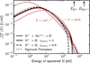 |
Fig. 5 Energy distribution of hydrogen atoms sputtered by 300 km/s solar wind H+ and He++ ions impacting the lunar regolith (the energies of the projectiles are marked by an upward arrow). All curves are computed with a surface binding energy for hydrogen of U = 5 eV, except for the thin red lines, which illustrate the effect of varying U on the energy distribution. Four models are shown: proton-induced sputtering without extra energy loss (solid black line); proton-induced sputtering with extra energy loss (dashed black line); sputtering from both protons and alpha particles, assuming an alpha-to-proton ratio of 4% and no extra energy loss (red solid line, with the thin red lines the same model computed for U = 1 eV and 10 eV); and the modified SigmundThompson model as defined by Wurz et al. (2022, Eq. (25)) calculated for a proton-induced sputtering of hydrogen. |
4.8 The scattered component
The energy distribution of light ions scattered from heavy materials has been extensively studied, particularly in the context of plasma-wall interactions in nuclear fusion reactors. At projectile energies of a few keV or lower, scattering occurs under two main regimes: single-collisional, dominating the high-energy end of the spectrum, and multiple-collisional, dominating the low-energy end. Tolmachev (1999) modelled light-ion scattering using a single-collision approach that includes both elastic and inelastic losses. Their model is versatile, as it applies to any ratio of the mean free path between elastic collisions to the total inelastic range.
In the energy region where multiple-collisions dominate, most theoretical models are derived by approximating the Boltzmann diffusion equation using various methods. Littmark & Gras-Marti (1978) addressed light-ion scattering by approximating the ion depth distribution using the method of moments. A particular result is that neglecting the skewness of the depth distribution yields a Gaussian approximation of the energy distribution of scattered particles. An alternative study from Forlano et al. (1996) used the discrete-streams method, assuming a power-law scattering cross-section and neglecting inelastic losses. Their model successfully predicts the characteristic double-peak energy distribution observed for light ions scattered from heavy targets: the higher-energy peak corresponds to particles that undergo only a few collisions, whereas the lower-energy peak arises from the multiple-collision regime (Brötzner et al. 2026). A later study by Falcone et al. (1999) included inelastic losses but neglected elastic ones, an assumption valid for light-ions scattered from heavy targets (Berger et al. 2005). This model shows good agreement with simulations, except for scattered ions with energies close to the incident energy, where the authors argue that adding elastic losses and fluctuations in inelastic losses would likely improve the agreement. Sukhomlinov (1997) treated the elastic losses in a perturbative expansion to linearise the Boltzmann diffusion equation. Their model considers a realistic multi-component, inhomogeneous material, and they showed that increasing density with depth reduces backscattering of high-energy ions (deeper penetration, multiple scattering) but increases it for low-energy ions (shallow penetration, single scattering).
More recently, Afanas’ev & Lobanova (2025) showed that the theory of electron scattering is applicable for describing the scattering of light ions and shows a particular good agreement with simulations for projectiles with energies in the keV range and above.
After considering all aforementioned analytical models, we chose the model of Forlano et al. (1996) for its simplicity and adaptability for fitting purposes. Figure 6 summarises the different stages of the scattering process considered in our model.
4.8.1 Adding inelastic losses
The model of Forlano et al. (1996) considers ions that impact a surface at normal incidence and scatter outward as a result of elastic binary collisions with surface atoms.
Inelastic energy losses are neglected in the original model by Forlano et al. (1996). We include inelastic energy losses (yellow overlay in Fig. 6) by modifying the high-energy asymptotic limit of the model. In the discrete-streams formalism, the quantity F2(z = 0, s ≫ 1) (Forlano et al. 1996, Eqs. (6) and (16)) is the Mellin transform (for example, Bertrand et al. 2000) of the energy distribution at depth z = 0 of particles backscattering with the highest energies (s ≫ 1). These particles follow the most efficient path consisting of only two elastic collisions with surface atoms (given an average scattering angle of 45°) to reverse from normal incidence, resulting in a maximum elastic energy of p2Ein, with p the relative energy loss during an elastic binary-collision. We model inelastic losses by reducing this cutoff energy to p2Ein – Δ∊, where Δe is the total inelastic energy loss for particles on this direct trajectory. This leads to a modified asymptotic expression (Forlano et al. 1996, see Eq. (16)):
 (25)
(25)
where the proportionality constant, describing the nuclear scattering probability, remains unchanged. This modification only affects the high-energy part of the distribution, and preserves the analytical form of the original solution. More practically, and for the case of velocity-proportional stopping power  (see Eq. (20)) that varies slowly at high energies, we can express Δ∊ ≈ neff Se (Ein) Leff, with neff the mean atomic number density of the regolith, and Leff the path length of this two-collisions scattering trajectory. By including this additional loss factor, the energy distribution of a projectile P scattering from a single-species surface of atoms S can be expressed as
![Mathematical equation: \mathcal{J}_E^{\mathrm{sc}}\left(E;E_\mathrm{in}, U,\Delta_\epsilon\right) &= \begin{cases} \dfrac{2E\kappa}{\mathtt{n}\left(E+U\right)^2} f\left(x\right),\quad &\text{if } x > 0 \\[.4cm] 0, \quad &\text{otherwise},\\ \end{cases}](/articles/aa/full_html/2026/06/aa59499-26/aa59499-26-eq48.png) (26a)
(26a)
 (26b)
(26b)
 (26c)
(26c)
 (26d)
(26d)
 (26e)
(26e)
where I2 is the modified Bessel function of the first kind; γ is the maximum fraction of energy transferred from a projectile to a surface atom during a single elastic collision as defined in Eq. (15); U is the surface binding energy; and m a factor that controls the power-law scattering cross-section as given by Eq. (29). To improve readability, we omitted the subscript (P → S) for p, m, Δ∊, and γ in Eqs. (26d) and (26e). The constant p(P→S) defines the relative energy lost during a single elastic collision that deflected the projectile by 45°, and is defined as in Forlano et al. (1996, Eq. (8)):
 (27)
(27)
The constant n normalises the function to unity, such that  . To reduce the computational cost of estimating the constant n via numerical integration, we evaluate it in an energy-normalised space, for which an approximate solution is provided in Appendix E. The function f is computationally expensive, but can be well approximated for 10−5 < x < 102 with a maximum relative error of 4% by:
 (28)
(28)
 |
Fig. 6 Schematised scattering of light ions from a surface. A proton (red filled circle) directed towards the surface: (1) rapidly neutralises; (2) scatter at small-to-medium angles off at least two surface atoms (black filled circles); (3) loses energy inelastically (yellow overlay); (4) exits the surface while charge-exchange transfers (green arrows) may lead to a final negative charge state (blue filled circle). |
4.8.2 Elastic scattering
Forlano et al. (1996) approximates the interatomic potential by a power law controlled by the exponent m = 1/s, with m as used in Eq. (26e), and s as defined in Lindhard et al. (1968, Eq. (3.5)). The special value m = 1 describes the case of hard-sphere interaction, where electronic screening is negligible and the scattering approaches a pure Rutherford-type interaction, well-represented by the unscreened Coulomb potential (Lindhard et al. 1968, Fig. 1). In the case of a light projectile with an energy of hundreds of eV impacting on a heavier material, electronic screening cannot be neglected, that is m < 1. We calculate the exponent m(P→S) (Ein) for a projectile (MP, ZP) at energy Ein impacting a surface atom (Ms, ZS) as
![Mathematical equation: m = 0.5 \left[1-\dfrac{\mathrm{d}\ln s_\mathrm{r}\left(\epsilon\right)}{\mathrm{d}\ln\epsilon}\right],](/articles/aa/full_html/2026/06/aa59499-26/aa59499-26-eq56.png) (29)
(29)
where sr(∊) is the reduced nuclear stopping cross-section (Lindhard et al. 1968, Eq. (4.11)), while e is the reduced energy (see Eq. (16)) evaluated at Ein. We calculate sr using the Krypton-Carbon potential, well approximated by Ziegler & Biersack (1985, Eq. (14)). Deriving sr from a Thomas-Fermi potential (Lindhard et al. 1968, Fig. 2, Table 2b) gives very similar results.
To approximate the exponent m for a hydrogen atom interacting with the multiple atomic species in the lunar regolith, we calculate an effective value as
 (30)
(30)
where rS is the atomic fraction of species S in the lunar regolith, as listed in Table 2. For a projectile energy of 470 eV (300km/s), we obtain m(H→eff) ≈ 0.57, and for 1300 eV (about 500km/s), m(H→eff) ≈ 0.66. As the projectile energy increases, the interatomic potential exponent m approaches unity, consistent with a transition towards hard sphere-like nuclear interactions.
4.8.3 Energy straggling
When a beam of mono-energetic ions travels through a material, individual ions do not lose the same amount of energy Δ∊ through inelastic collisions. Instead, the inelastic energy loss follows a statistical distribution with mean μ∊ and a width characterised by the standard deviation, σ∊. We refer to this width as energy straggling.
The energy straggling is caused by statistical fluctuations in the inelastic collision processes. Kaneko (1990) showed that the excitation of outer-shell electrons plays an important role in the energy loss of slow ions. Using a shell-wise local electron density model for hydrogen-lead interactions, they reported (Kaneko 1990, Table 1) that the 6s and 6p shells dominate inelastic losses at low velocities, with relative straggling σ∊/μ∊ of 16% and 11%, respectively. Inner shells contribute much less to the total energy loss at low velocities because slow projectiles rarely penetrate deeply enough to interact with them. Nevertheless, when such interactions do occur, the associated energy straggling can be large. For example, the straggling associated with the 2s shell is large, σ∊/μ∊ = 560%. The lunar regolith is primarily composed of oxygen atoms, whose electronic configuration 1s22s22p4 involves only such inner shells, all of which are associated with large energy straggling.
To introduce the energy straggling in our model, we treat Δ∊ as a random variable drawn from a normal distribution truncated to the physically-allowed interval 0 ≤ Δ∊ < Δ∊max, with Δ∊max = p2(Ein + U) – U derived from the condition x > 0 (see Eq. (26)), expressed as
 (31)
(31)
The expected value of the energy distribution  over the truncated Gaussian can be expressed as
![Mathematical equation: \mathbb{E}\left[ \mathcal{J}_E^{\mathrm{sc}}\left(E; \Delta_\epsilon\right) \right] &= \frac{1}{Z\sqrt{\pi}} \int_{t_0}^{t_1} \mathcal{J}_E^{\mathrm{sc}}\left(E;\Delta_\epsilon= \mu_\epsilon + \sqrt{2} \sigma_\epsilon t\right) e^{-t^2} \mathrm{d}t, \\](/articles/aa/full_html/2026/06/aa59499-26/aa59499-26-eq60.png) (32a)
(32a)
 (32b)
(32b)
 (32c)
(32c)
 (32d)
(32d)
where erf is the error function, and t the integration variable. In practice, this integral is evaluated numerically using the Gauss-Legendre quadrature restricted to the interval [t0,t1]:
![Mathematical equation: \mathbb{E}\left[ \mathcal{J}_E^{\mathrm{sc}}\left(E; \Delta_\epsilon\right) \right] &\approx \frac{t_1-t_0}{Z\sqrt{\pi}} \sum_i^N w_i \,\mathcal{J}_E^{\mathrm{sc}}\left(E, \Delta_\epsilon=\mu_\epsilon + \sqrt{2} \sigma_\epsilon t_i\right) e^{-t_i^2}, \\](/articles/aa/full_html/2026/06/aa59499-26/aa59499-26-eq64.png) (33a)
(33a)
 (33b)
(33b)
where ri and wi are the i-th Gauss-Legendre root and weight of the N-th Legendre polynomial, respectively. For a sufficiently large N, the property ![Mathematical equation: $\int_0^\infty \mathbb{E}\left[ \mathcal{J}_E^{\mathrm{sc}}\left(E; \Delta_\epsilon\right) \right] \mathrm{d}E = 1$](/articles/aa/full_html/2026/06/aa59499-26/aa59499-26-eq66.png) is conserved. To make the notation clear, we write the energy distribution of a projectile P that scatters from surface atoms S as
is conserved. To make the notation clear, we write the energy distribution of a projectile P that scatters from surface atoms S as
![Mathematical equation: \mathcal{J}_{\left(\mathrm{P}\rightarrow\mathrm{S}\right)}^{\mathrm{sc}}\left(E;E_\mathrm{in}, U,\mu_\epsilon, \sigma_\epsilon\right) = \mathbb{E}\left[ \mathcal{J}_E^{\mathrm{sc}}\left(E;E_\mathrm{in}, U,\Delta_\epsilon\right) \right] .](/articles/aa/full_html/2026/06/aa59499-26/aa59499-26-eq67.png) (34)
(34)
4.8.4 Multi-species surface
To extend the model from Forlano et al. (1996) to a multi-species surface, a rigorous approach would be to modify the energy transfer function K in Forlano et al. (1996, Eq. (1)). However, to preserve the analytical traceability of the original solution, we decided to weight the contribution of each atomic species to the reflection process by directly weighting Eq. (34), that is,
 (35)
(35)
with  , where Sn is proportional (up to a species-independent factor) to the nuclear stopping power. This weighting is analogous to the species-dependent weighting factor used in Eckstein & Preuss (2003) when modelling the energy dependence of sputtering yields. Sn is defined as (Wilson et al. 1977, Eq. (9))
![Mathematical equation: S_n^{\left(\mathrm{P}\rightarrow \mathrm{S}\right)}\left(E\right) \propto \dfrac{M_\mathrm{P} Z_\mathrm{P} Z_\mathrm{S}}{\left(M_\mathrm{P} + M_\mathrm{S}\right) \sqrt{Z_\mathrm{P}^{2/3}+Z_\mathrm{S}^{2/3}}} s_\mathrm{r}\left[\epsilon_{\left(\mathrm{P}\rightarrow \mathrm{S}\right)}\left(E\right)\right].](/articles/aa/full_html/2026/06/aa59499-26/aa59499-26-eq70.png) (36)
(36)
Weighting by the nuclear stopping power encodes the fraction of the total nuclear stopping power contributed by species S, directly reflecting its ability to deflect an incoming particle, P.
Table 2 lists, for a hydrogen atom as projectile, the nuclear stopping power, up to a constant, of the atomic elements that make up the lunar regolith. The values range from 5.08 to 6.88. Lighter elements show higher stopping powers, meaning they are more effective at deflecting hydrogen. Therefore, species heavier than oxygen, which dominates the atomic composition, play a minor role, both because of their lower abundance and their reduced ability to deflect hydrogen. Therefore, describing the surface as composed of a single effective species is reasonable,
 (37)
(37)
with Seff = (Meff, Zeff) defining the averaged atomic mass and atomic number of the lunar regolith, weighted by their atomic abundance. From Table 2, we get Seff = (21.88 amu, 10.81).
4.8.5 Constraining the model with simulations
The two main unknown parameters in our model are the mean inelastic energy loss, μ∊, and the energy loss straggling, σ∊. The two quantities constrain the inelastic energy loss, Δ∊, that is the total energy lost inelastically by a particle as it travels through a material. A longer path length within the material leads to a greater total loss. We approximate the dependence of Δ∊ on the path length of a particle in the material by expressing it as a function of the total scattering angle, Ψ. We define the total scattering angle as the angle between the incident particle direction and the emission direction (see Fig. 2). Its relation to the incident and emission angles is
![Mathematical equation: \Psi= \pi - \arccos{\big[\cos{\left(\mathrm{SZA}\right)}\cos{\left(\beta\right)}+\sin{\left(\mathrm{SZA}\right)}\sin{\left(\beta\right)}\cos{\left(\phi\right)}\big]},](/articles/aa/full_html/2026/06/aa59499-26/aa59499-26-eq72.png) (38)
(38)
with Ψ, SZA, φ and β all in radians. For a particle that reverses its direction completely - backscattering along the incident path - the scattering angle is Ψ = 180°. Scattering at a grazing incidence and emission corresponds to Ψ ≈ 0°. A larger scattering angle implies a longer path length within the material -a particle that reverses its direction of motion is likely to suffer many collisions, leading to a longer path length.
The total inelastic energy loss must also depend on the energy of the projectile, which increases with increasing incident energy. Therefore, we aim to parametrise μ∊ (Ein, Ψ) and σ (Ein, Ψ). To do so, we compare and constrain our models with SDTrimSP-3D simulations of solar wind protons scattering from a rough surface representing lunar regolith (Szabo et al. 2023b). These simulations aim at reproducing the energy dependence of the differential flux of emitted energetic neutral hydrogen atoms from the lunar surface and show good agreement with observations from the Chandrayaan-1 Energetic Neutral Analyzer (CENA) instrument (Barabash et al. 2009). We first constrained the dependence on the total scattering angle using simulation results from Szabo et al. (2023a, Figs. 4 and 7). Then we constrained the dependence on the energy of the incident particle using Szabo et al. (2023a, Fig. 5b).
4.8.6 Angular-dependence of the inelastic loss and straggling
We constrained the angular dependence using simulations from Szabo et al. (2023a, Figs. 4 and 7), which show the energy distributions of protons scattered from a regolith-like surface as functions of the macroscopic emission angle β. The simulation data cover two different SZA values: 0° and 60°.
We fit the parameters (μ∊,σ∊) in our model to match the simulated energy distributions for all available combinations of SZA and β, summarised by the total scattering angle Ψ. Figure 7 compares our fitted model with the simulated spectra. We show, for comparison, models with (Eq. (34)) and without (Eq. (26)) energy straggling, and the original model of Forlano et al. (1996).
Our model reproduces the simulated spectra well, except for total scattering angles smaller than about 100°. In this regime illustrated in Fig. 7a, the original model of Forlano et al. (1996) already overestimates the energy loss, and adding an inelastic energy loss term further degrades the fit. A likely explanation for this poorer agreement at Ψ < 100° is that the model from Forlano et al. (1996) was formulated for particles incident normal to the surface and scattering away from it, thereby restricting the scattering angle to Ψ ∊ [90°, 180°]. The model is not derived for smaller scattering angles.
In a second step, we fit the parameters (μ∊, σ∊) obtained from fitting the simulated spectra in Fig. 7 as a function of Ψ. For μ∊ we obtain the fit presented in Fig. 8. From this study, we find that the mean inelastic energy loss, μ∊ [eV], shows a sigmoid-curve dependence on the scattering angle, Ψ [deg], given by:
![Mathematical equation: \mu_\epsilon\left(\Psi, E_\mathrm{in}=470\;\mathrm{eV}\right) \approx 94.6 \; \Big\{1+\exp\left[-0.0588 \left(\Psi - 90\right)\right]\Big\}^{-2.03}.](/articles/aa/full_html/2026/06/aa59499-26/aa59499-26-eq73.png) (39)
(39)
We observed that a constant relative energy loss straggling of σ∊ = 0.7μ∊ fits the simulation data well.
4.8.7 Energy dependence between the inelastic energy loss and straggling
The inelastic energy loss depends on the projectile energy: as the projectile energy increases, the particle loses more energy through inelastic processes (see Eq. (20)) and generally travels longer within a material. In this section, we fit the mean inelastic energy loss, μ∊, and the energy loss straggling, σ∊, of our model to the data presented in Szabo et al. (2023b, Figs. 4 and 5), corresponding to scattering angles Ψ > 160°. These data are then used to constrain the amplitude of Eq. (39) as a function of the projectile energy. The fitted models, together with the simulated energy spectra, are shown in Fig. 9, and the resulting model parameters are summarised in Table 1.
The model fits the simulated data reasonably well. The high-energy peak is accurately reproduced, while discrepancies appear at low energies corresponding to the multiple-scattering regime. One possible reason is that inelastic losses are included in our model only for particles scattering after a small number of collisions (s ≫ 1 in Eq. (25)). As a result, inelastic losses in the multiple-scattering regime are likely underestimated.
Based on the data of Table 1, we generalised the mean inelastic energy loss model of Eq. (39) to arbitrary incident energies by scaling the amplitude with energy. This yields the relation
![Mathematical equation: \mu_\epsilon\left(\Psi, E_\mathrm{in}\right) = \mathrm{A}_{470} \left(\dfrac{E_\mathrm{in}}{470}\right)^{k_0} \cdot \Big\{1+\exp\left[-k_1 \left(\Psi - 90\right)\right]\Big\}^{-k_2},](/articles/aa/full_html/2026/06/aa59499-26/aa59499-26-eq74.png) (40)
(40)
with fit parameters A470 = 94.6 [eV], k0 = 1.44, k1 = 0.0588 [1/deg], and k2 = 2.03. The exponent k0 is kept a fixed constant throughout this paper. At low energies, inelastic losses are typically proportional to the projectile velocity (Sect. 4.7.3), corresponding to k0 = 0.5. In contrast, our fit yields a much steeper dependence (k0 ≈ 1.5), which can be understood as higher-energy projectiles travel longer distances within the material, leading to larger total inelastic losses. We found that a constant relative energy loss straggling of 65% fits the simulated spectra well. This is expressed as
 (41)
(41)
Simulations by Szabo et al. (2023b) show that electronic stopping represents the dominant energy loss mechanism for protons with typical solar wind energies scattering off lunar regolith, accounting for approximately 65% of the total energy loss for 300 km/s protons. We find a similar result: from Equation (40) and for Ein = 470 eV (as an example), the maximum inelastic energy loss is about 90 eV. In the single-collision regime (Eq. (25)), the minimum energy loss is given by p2Ein –Δ∊, where Δ∊ ≈ 90 eV corresponds to 71% of the total energy loss for Ein = 470 eV. For particles contributing to the high-energy peaks in Fig. 9, inelastic losses account for roughly 50% of the total energy losses.
We can approximate the shortest path length of scattered protons using the following relationship: ![Mathematical equation: $L_{\mathrm{eff}} \approx \Delta_\epsilon/\left[ n_\mathrm{eff}\cdot S_e\left(E_\mathrm{in}\right)\right]$](/articles/aa/full_html/2026/06/aa59499-26/aa59499-26-eq76.png) (see Section 4.8.1). Assuming an averaged electronic stopping power of Se ≈ 0.2 eV nm2 (obtained from Eq. (20) for an averaged regolith atomic number of 10.81 and for Ein = 470 eV), a regolith grain number density of approximately n = 83 atoms/nm3 (assuming a grain density of 3.035 g/cm3 (Li et al. 2024) and an averaged molar mass of about 22 g/mol), and a total inelastic loss of 90 eV (for near 180°-backscattering protons), we obtain Leff ≈ 5.4 nm. Tucker et al. (2019) showed that solar wind implants protons into the top 20-30 nm of lunar regolith grains, a range consistent with our estimated path length. The estimated path length is also comparable to the hydrogen enhancement depth observed in regolith samples returned by Chang'e5 (Zhou et al. 2022).
(see Section 4.8.1). Assuming an averaged electronic stopping power of Se ≈ 0.2 eV nm2 (obtained from Eq. (20) for an averaged regolith atomic number of 10.81 and for Ein = 470 eV), a regolith grain number density of approximately n = 83 atoms/nm3 (assuming a grain density of 3.035 g/cm3 (Li et al. 2024) and an averaged molar mass of about 22 g/mol), and a total inelastic loss of 90 eV (for near 180°-backscattering protons), we obtain Leff ≈ 5.4 nm. Tucker et al. (2019) showed that solar wind implants protons into the top 20-30 nm of lunar regolith grains, a range consistent with our estimated path length. The estimated path length is also comparable to the hydrogen enhancement depth observed in regolith samples returned by Chang'e5 (Zhou et al. 2022).
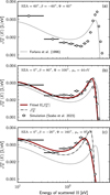 |
Fig. 7 Comparison of our energy distribution model with simulation data for 300 km/s solar wind protons (470 eV) scattering off lunar regolith at three different scattering angles. Panels a-c show the fitted model for three different total scattering angles Φ = 60°, 100°, and 160°, respectively. The original model from Forlano et al. (1996) in panel a provides a reasonable match to the simulation data but generally overestimates the energy loss. The energy straggling is set to σ∊ = 0.7 μ∊. For both panels b and c: the original model (dotted line) from Forlano et al. (1996) provides a reasonable average fit but consistently overestimates the energy of the high-energy scattered population. The modified model (Eq. (26); dash-dotted line), which includes a constant inelastic loss, improves the fit, though it underestimates the width of the high-energy peak at large scattering angles. Including energy loss straggling (Eq. (34), red solid line) further improves the fit. All comparisons use a surface binding energy of U = 5 eV. Note that in panel a) only one line (dotted) is shown as all three models coincide. |
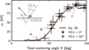 |
Fig. 8 Relation between the mean inelastic energy loss, μ∊, and the total scattering angle, Ψ. The mean inelastic energy loss is fitted for different SZA values (crosses: normal incidence; circles: 60° incidence) and for various emission angles. Crosses are shifted by −5° for clarity. Equation (39) is shown as the solid red line. The fits from the three panels in Fig. 7 are labelled. |
 |
Fig. 9 Comparison between the energy distribution model (Eq. (34) solid lines) and simulated energy distributions (open circles) of solar wind proton scattering at normal incidence on the lunar regolith for proton incident speeds of 300 km/s (blue) and 500 km/s (red) (Szabo et al. 2023b, Figs. 4 and 5). The thick lines show models computed with a surface binding energy of U = 5 eV. Varying U primarily affects the low-energy tail of the distribution, as illustrated by the thin blue lines, which span U = 1-10 eV. |
Parametrisation of the energy distribution model.
5 Application to data
The NILS data report the differential number flux of negative hydrogen ions emitted from the lunar surface as a result of precipitating solar wind ions. The observed flux, denoted as J−H, depends on the properties of the precipitating flux, which varies moderately over the course of the NILS mission (Wieser et al. 2025). In the following, we briefly assess the impact of these variations and state the simplifying assumptions adopted in our model.
During the mission, the SZA varied from 52° to 47°; a minimal variation over which we do not expect a significant change in J−H. For example, Brötzner et al. (2025) showed that the sputtering yield is largely independent of the angle of incidence. The angular distribution of the scattering and/or sputtering depends on the SZA (Schaufelberger et al. 2011), although we neglect any dependencies on the SZA but in the estimation of f⊥ and the inelastic energy loss model.
Similarly, the speed of the solar wind vsw varied between 290 km/s and 310 km/s. The yield ηsc depends on the incident energy of the solar wind protons and decreases with increasing energy (Lue et al. 2018, Fig. 6b), likely because deeper penetration reduces the probability of escape. Similarly, the sputtering yield depends on the precipitating energy. Nevertheless, given the restricted speed range covered during the NILS mission, we approximate ηsc (Esw) and ηsp (Esw) as constants ηsc and ηsp.
The SAA (Fig. 2) angle varied from 43°E to 28°E, a total change of 15°. The NILS instrument provides an azimuthal coverage of approximately 15° (Canu-Blot et al. 2025, see Δα in Table 3), which is comparable to this variation. Therefore, all quantities are given for an average azimuthal emission angle of φ = 213° (see Appendix C for further details).
As indicated in Sect. 4.7.6, alpha particles are more efficient at sputtering hydrogen than solar wind protons. Although alpha particles do not significantly affect the energy distribution of sputtered hydrogen atoms, neglecting their contribution would underestimate the sputtered flux. We therefore account for their presence by scaling the precipitating proton flux with a correction factor, kα, determined in in Sect. 4.7.6.
Starting from Eq. (12), we therefore replace various quantities by their average values, explicitly state all dependences on the model parameters, and describe the observed negative ion flux as seen by NILS as
![Mathematical equation: \begin{split} \mathcal{J}^-_\mathrm{H}&\left(E,\beta,\overline{\phi}\right) \, = \\ &\mathrm{P}^-\left(v_\perp;v_\perp^{50\%},k\right) f_{\mathrm{sw}} \cos\left(\mathrm{SZA}\right)\cdot\\ &\big\{\\ &\quad\mathcal{J}_E^\mathrm{sp}\left(E;E_\mathrm{in}, U, \gamma_{\mathrm{extra}}\right)\; \left[\left(1+k_\alpha\right) \;\overline{\eta^\mathrm{sp}} \; \mathcal{J}_{\Omega}^\mathrm{sp}\left(\beta,\overline{\phi}\right)\right] \\ &+\\ &\quad\mathcal{J}_E^\mathrm{sc}\left(E;E_\mathrm{in}, U, \mu_\epsilon, \sigma_\epsilon \right) \; \left[\overline{\eta^\mathrm{sc}} \; \mathcal{J}_{\Omega}^\mathrm{sc}\left(\beta,\overline{\phi}\right)\right]\\ &\big\},\\ \end{split}](/articles/aa/full_html/2026/06/aa59499-26/aa59499-26-eq77.png) (42)
(42)
with Ein = Esw;  , where mH is the proton mass and β′ the microscopic polar emission angle; μ. = μ∊ (Ψ, Ein; A470, k1, k2); σ∊ = 0.7μ∊; Ψ = Ψ (SZA, β, ϕ); and kα = 0.11.
5.1 Additional prior knowledge needed
The model in Eq. (42) depends on the surface binding energy, U, and the scattering and sputtering angular distributions (three quantities which are not well-constrained by the limited NILS data). Additionally, the model is close to non-identifiable (Raue et al. 2009) as both the scattering and sputtering yields along with the probability of negative ionisation influence the amplitude of the differential flux. A model is said to be non-identifiable when two or more parametrisations are observationally identical. We alleviate the non-identifiability issue and missing knowledge by statistically adding prior information, as described in the following sections.
We evaluated all priors using a prior predictive check (Gelman 2014) by sampling from the joint prior  , propagating these samples through the model, and examining the resulting prior-predictive flux distribution. This ensured that the priors produced physically-plausible fluxes.
5.1.1 Surface binding energy
The surface binding energy U of hydrogen atoms in regolith depends on the regolith base composition and absorbed species (hydroxylation of the regolith may affect the surface binding energy). We softly constrain the surface binding energy, shared by both the sputtering and scattering models, by using a truncated normal distribution (TruncNorm) as a prior distribution,
 (43)
(43)
where all parameters are in units of eV. The probability is set to 0 for U ≤ 0. We set the average prior knowledge to 5 eV as it was successfully used in the earlier model of Wieser et al. (2024).
5.1.2 Energetic neutral hydrogen albedo
As stated in Sect. 5.1, the model in Eq. (42) has an identifiability issue, as both the scattering and sputtering yields and the probability of negative ionisation influence the amplitude of the differential flux. The limited energy and angular coverage of the NILS data further complicate making a distinction between the individual contributions.
To address this identifiability issue, we add the knowledge of a global lunar energetic neutral hydrogen albedo ηENA of 0.16 ± 0.05, as derived in Vorburger et al. (2013). The study of Vorburger et al. (2013) defines energetic neutral hydrogen atoms as hydrogen emitted from the lunar surface with energies above 11 eV. We define this albedo using our model based on the following assumptions:
- (1)
The albedo values reported by Vorburger et al. (2013) are derived from the full observation of both angular distributions,
 and
and  .
. - (2)
The neutralisation probability, P0, is assumed to be independent of both the emission energy and emission direction. Naturally, this cannot be the case, since P0 ≈ 1 – P− and P−depends on v⊥. However, this approximation is still deemed reasonable as Wieser et al. (2024) successfully predicted the energy distribution of the differential flux of neutral hydrogen atoms emitted from the lunar surface using the physical model of Kenmotsu et al. (2004), without considering any ionisation probability. That model is closely related to the model of Ono et al. (2005) adopted in the present study.
- (3)
The probability of positive ionisation is small compared to the probability of neutralisation. Lue et al. (2018, Fig. 6a) reported a charge ratio H+/H0 of approximately 5% for hydrogen emitted at speeds similar as in our study. The ratio is derived from orbital observation, at an altitude at which we can assume all negative hydrogen ions have been converted to neutrals. We therefore write P+ ≪ P0 + P− and P0 ≈ 1 – P−.
Based on the assumptions above, from Eq. (12), we obtain
![Mathematical equation: \eta^\mathrm{ENA} \equiv \mathrm{P}^0 \int_{11 \;\left[\mathrm{eV}\right]}^\infty \left[\eta^\mathrm{sc} \mathcal{J}_E^\mathrm{sc} + \left(1+k_\alpha\right) \;\eta^\mathrm{sp} \mathcal{J}_E^\mathrm{sp}\right]\mathrm{d}E,](/articles/aa/full_html/2026/06/aa59499-26/aa59499-26-eq83.png) (44)
(44)
with P0 = 1 – P−, where P− is reduced to a constant equal to the average of P− (v⊥) for v⊥ ranging from 104 m/s to 105 m/s. We added a constant kα = 0.11 to account for the alpha-induced sputtering, as in Eq. (42).
Practically, Vorburger et al. (2013) were not able to reliably observe neutral hydrogen atoms with energies below 11 eV.
Using Eq. (44), we estimate the fraction of the total scattered and sputtered energetic neutral hydrogen observed by Vorburger et al. (2013) to be 97% and 59%, respectively (assuming a binding energy of 5 eV). Increasing the energy cut-off to 20 eV reduces the observed sputtering fraction to 40%; we nevertheless keep the cut-off of 11 eV to be able to compare results. Across the range of solar wind speeds considered (300-500 km/s), the estimates change only by 3%, a minimal variation that we neglect. The surface binding energy has the largest influence. However, varying it from 2 to 8 eV changes the estimate by only about ±15%. We therefore neglect this effect as well to lower the complexity of the model. This leads to the following prior parametrisation of the yields
 (45a)
(45a)
 (45b)
(45b)
 (45c)
(45c)
 (45d)
(45d)
 (45e)
(45e)
where Uniform is a uniform distribution between the two given boundaries.
5.1.3 Angular prior distributions
All quantities in the model of Eq. (42) are either known or statistically constrained by prior information, with the exception of the angular emission profiles  (β, φ) and
  (β, φ).
The NILS instrument observed the lunar surface using an electrostatically-steerable angular pixel. The angular coverage of the surface is divided into eight intervals and covers emission polar angles from βmax = 90° (horizon-looking from the instrument perspective) to βmin = 45° (downward-looking from the instrument perspective). This angular scanning allows for extraction of information about the emission profiles from the NILS data. In the following, we statistically encode prior information of the scattered/sputtered emission profiles.
Scattering. Prior knowledge of the angular distribution of scattered particles from the lunar surface is available from the simulation results of Szabo et al. (2023b, Fig. 1). Their simulated profile was obtained for SZA values between 60° and 75°, close to the average SZA of 50° during the NILS mission. We parametrised this prior distribution as
![Mathematical equation: &\mathcal{J}_\Omega^\text{sc, prior}\left(\beta\right) = \dfrac{f\left(\beta\right)}{2\pi}\;,\\[0.5cm]](/articles/aa/full_html/2026/06/aa59499-26/aa59499-26-eq91.png) (46a)
(46a)
 (46b)
(46b)
with β defined as in Szabo et al. (2023b), that is, ranging from –π/2 to π/2, with forward-scattering for β > 0 and backwardscattering (towards the Sun) for β < 0. The profile is tilted such that about 40% of emitted particles are forward-scattered. The NILS instrument observed the less-likely forward-scattering component of the emission profile, which is accounted for in the calculation of the total scattering yield.
Sputtering. Cassidy & Johnson (2005) simulated the sputtering of atoms from a porous regolith and showed that the angular emission of sputtered particles differs only little from that of a smooth surface. In both cases, the emission follows a cosinelaw distribution. Alternatively, Jäggi et al. (2024) showed that for oblique incidence of precipitating solar wind protons onto regolith-like surfaces, sputtering of heavy elements (for example, oxygen) is preferentially forward-directed, that is, along the solar wind flow. However, we expect hydrogen recoils to be produced nearly isotropically because the projectile and target masses are identical. Accordingly, we adopt a priori the following angular distribution:
 (47)
(47)
5.2 The near-surface lunar environment
Particle emission from lunar regolith is modulated by environmental parameters such as regolith composition at the landing site, local topography, surface disturbances caused by the lander, solar wind plasma conditions, and nearby magnetic anomalies. In the following section, we discuss how each of these factors affects the analysis of NILS data.
5.2.1 Effect of the solar wind parameters
We model the solar wind proton energy as Gaussian-distributed, with the mean equal to the bulk energy. The temperature of solar wind protons affects the precipitating energy distribution, which leads, to the first-order, to a broadening of the scattered/sputtered energy distributions.
Following Szabo et al. (2023b, Eq. (3)), the standard deviation can be approximated as  , with kBTsw ≈ 1.5 eV for vsw = 300 km/s, as expressed in Szabo et al. (2023b, Eq. (4)).
We find that for solar wind speed between 300 km/s and 500 km/s, the temperature has only a minor effect on the energy distribution of scattered/sputtered particles. Such an effect is neglected, and we thereafter treat solar wind protons as mono-energetic. We additionally assume a uniform solar wind, such that all protons impinge on the surface at a constant SZA, approximated by the Sun direction, ignoring any aberration. We note that the Moon was outside of Earth’s bow shock in undisturbed solar wind during the time NILS recorded data. We also neglect any heating from lunar magnetic anomalies as well as a possible deflection of the solar wind flow direction before it impinges onto the surface.
5.2.2 Possible effects of lunar magnetic anomalies
The Chang’e-6 landing site is located west of a large cluster of lunar crustal magnetic anomalies near the South Pole-Aitken (SPA) basin. The direct interaction between the lunar crustal fields and the solar wind deflects and reflects incident solar wind protons (Futaana 2003; Lue et al. 2011), reducing proton precipitation within magnetic anomalies and enhancing it in surrounding regions (Wieser et al. 2010; Vorburger et al. 2013; Fatemi et al. 2015; Maynadié et al. 2025). The magnetic anomaly cluster near the SPA basin is the largest and among the strongest magnetic anomalies on the Moon. The high reflected proton densities of the cluster generate macroscopic plasma disturbances (Halekas et al. 2014; Fatemi et al. 2014; Halekas et al. 2017) disturbing proton precipitation over thousands of kilometres around the cluster (Maynadié et al. 2025). As a result, the precipitating solar wind proton energies and fluxes at the Chang’e-6 landing may significantly differ from upstream conditions.
To investigate these effects, we model the energy and flux of solar wind protons impacting the lunar surface observed by NILS as
![Mathematical equation: \begin{align} f_\mathrm{sw} &= \nu_f \;f_\mathrm{sw}^\mathrm{up},\\[0.2cm] \end{align}](/articles/aa/full_html/2026/06/aa59499-26/aa59499-26-eq95.png) (48a)
(48a)
 (48b)
(48b)
where (fsw, Esw) are defined as in Eq. (42), and  are the undisturbed upstream solar wind flux and energy. Upstream solar wind parameters were obtained from measurements by the electrostatic analyzer (McFadden et al. 2008) onboard of the ARTEMIS-P2 spacecraft (Angelopoulos 2011). ARTEMIS-P2 was in an elliptic orbit around the moon at a distance of 103−104 km from NILS. The time-dependent multiplicative factors (νf,vE) quantifying the effect of magnetic anomalies on the upstream solar wind flux and energy are estimated in the following subsections.
Simplified model. The high-energy part of the scattered energy distribution mainly comprises of solar wind protons that have only experienced a few collisions with surface atoms. These reflected particles provide the most direct surface-originating proxy for the solar wind proton flux and energy impinging on the surface.
We constructed a simplified model for the high-energy (> 100 eV) negative hydrogen differential flux J−H emitted from the surface. We neglect the contribution from sputtering (minimal at these energies, as can be seen in Fig. 1) and assume a constant ionisation probability, P−, independently of the emission energy and angles. The simplified model can be expressed as
![Mathematical equation: \begin{split} \mathcal{J}_\mathrm{H}^-\left(E\right) \propto \; &\nu_f f_\mathrm{sw}^\mathrm{up} \cos\left(\mathrm{SZA}\right) \\[0.25cm] &\cdot \mathcal{J}_E^\mathrm{sc}\left[E; E_\mathrm{in} = \nu_\mathrm{E} E_\mathrm{sw}^\mathrm{up}, U, \mu_\epsilon, \sigma_\epsilon\right] \\[0.25cm] &\cdot \mathcal{J}^{\mathrm{sc,prior}}_\Omega, \end{split}](/articles/aa/full_html/2026/06/aa59499-26/aa59499-26-eq98.png) (49)
(49)
where the proportionality accounts for the scattering yield ηsc, and the probability of ionisation, P−, both of which do not affect the inference of the variations of the factor, νf, and can be factored out for simplicity. For simplicity, we model the angular distribution of scattered hydrogen atoms using the prior distribution defined by Eq. (46). The inelastic energy loss, μ∊, is simplified to a constant inferred from data, with an energy straggling of σ∊ = 0.7 μ∊ (Eq. (41)). The surface binding energy is set to U = 5 eV, as in Sect. 5.1.1. The factor, νf, is constrained by a weakly-informative prior (Table F.1) that adds the knowledge that magnetic anomalies are unlikely to more than double the upstream solar wind flux (Maynadié et al. 2025; Fatemi et al. 2015).
While Eq. (49) constrains the relative temporal variation of νf, its absolute value remains unconstrained because the model is expressed up to a proportionality constant. However, Maynadié et al. (2025, Fig. 3) showed that although magnetic anomalies significantly affect proton precipitation at the NILS location and the effect is highly variable and time-dependent, the average precipitating proton flux remains comparable to that in regions not influenced by magnetic anomalies. Therefore, we assume that the average of νf computed over the whole NILS mission - a duration of about one Earth day - provides a reasonable estimate for undisturbed solar wind conditions, that is, vf ≈ 1.
Inference from data. Figure 10 shows the observed negative hydrogen ion energy-differential flux originating from the surface, denoted as E J−H, normalised by the upstream flux  . If the solar wind was not affected by the lunar environment, no variation in the observed flux would be expected beyond that arising from counting statistics. However, this is not what is observed: some time segments (for example, 02T19:44) show low fluxes, whereas others (for example, 03T03:03) show high fluxes. These variations are well-reproduced by the factor νf, inferred from our simplified model.
Figure 10 also shows the energy distribution of the energydifferential flux. The distribution shows temporal shifts in energy, with lower mean energies at, for example, 03T03:31 and higher mean energies at, for example, 03T02:48. Nevertheless, the energy distribution is rather constant and bounded by the energy of upstream solar wind protons, as represented by the red line in the lower panel of Fig. 10. The factor νE could not be inferred due to non-identifiability versus νf. For simplicity, we fix νE = 1 hereafter. This approximation is justified by the limited magnitude of the observed energy shifts. The factor νE is likely less than one, that is, solar wind protons are systematically decelerated by magnetic anomalies. Such observation has already been reported by previous studies (Saito et al. 2012; Futaana et al. 2013; Fatemi et al. 2015).
We visually inspected the correlation between the scale factor νf and the following upstream conditions: solar wind proton density and speed; interplanetary magnetic field magnitude and direction. We did not observe any convincing correlation, supporting the idea of a turbulent propagation of the solar wind down to the surface.
5.2.3 Lunar regolith composition
The lunar soil at the landing position of Chang’e-6 shows a bulk density of 0.983 g/cm3 (Li et al. 2024), lower than most of Apollo, Luna, and Chang’e-5 samples, which typically ranges from 1.1 to 2.1 g/cm3. This suggests the Chang’e-6 lunar soil is more porous than previously visited soils. The average density of individual grains is similar than the Chang’e-5 mission, at a value of 3.035 g/cm3.
From the chemical composition of the CE6C0000YJFM00102 and CE6C0000YJFM00103 samples from Chang’e-6 (Li et al. 2024, Table 2), we derive the average elemental composition of the lunar regolith at the Chang’e-6 landing site. We calculated the relative atomic concentrations from the oxide weight percentages averaged over the two samples, assuming ideal stoichiometry and that all elements occur in the listed oxides. Beside the bulk composition, Lin et al. (2025) also measured the hydrogen content in the outermost surface layer of the Chang’e-6 lunar grains. This region is particularly important for our study because the solar wind interacts mainly with the top few tens of nanometres of the regolith grains. Their measurements show that the soil grains are enriched in hydrogen of solar wind origin within the upper 200 nm, with concentrations reaching up to 0.19 wt% (equivalent of 1.7 wt% H2O by weight), and increasing towards the surface. We add this extra solar wind-implanted hydrogen content to our regolith composition model, finally obtaining the first three columns of Table 2. The elemental composition derived from the Chang’e-6 samples closely matches that reported by Wieser et al. (2025, Table 2).
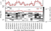 |
Fig. 10 Energy-time spectrogram of the negative hydrogen ions energy-differential flux at the surface, normalised by the upstream solar wind flux. The flux is expressed in units of 1/sr. The flux is averaged over angles. The time is discontinuous with each bin labelled by its average date (UTC). Upper panel: temporal variation of the solar wind flux enhancement and reduction factor, νf, with the red horizontal line the best estimate (at the maximum a posteriori) and the vertical error bars the uncertainty (68% highest density interval). Lower panel: the red solid line represents the upstream energy. Increases in the observed normalised flux are well reproduced by the model, corresponding to increases in the factor vf. |
Elemental composition of the regolith at the landing position of Chang’e-6.
5.2.4 Lunar topography
The terrain surrounding the Chang’e-6 landing site was reconstructed from Landing Camera (LCAM) images with a spatial resolution of 1 cm (Liu et al. 2025). The lander touched down on the rim of a 20 m-wide crater. Using the resulting elevation model (Fig. 11a), we calculated the macroscopic emission angle β as observed by the NILS instrument, which is mounted approximately 1.35 m above the surface. Figure 11b shows the emission angle β across the lander coordinate system defined in Canu-Blot et al. (2025, Fig. 8). The shown angle is an average over areas of 25 cm2. Despite the locally cratered terrain, the reconstructed polar emission angle differs only slightly from that of a flat surface. Across the NILS field of view, deviations from a flat surface remain within ±5°, indicating that a flat-surface approximation is reasonable for our analysis.
5.2.5 Regolith disturbances by the lander
The exhaust plume of the lander engines mechanically disturbs the upper regolith layers at the landing site. For Chang’e-5, Zhang et al. (2022) reported an erosion depth of approximately 0.2 cm, corresponding to a total eroded mass of about 336 kg, with disturbances extending up to 13 m from the landing location. A large fraction of the area sampled by NILS lies within this radius (Fig. 11a). Disturbed regolith is expected to show a modified grain-size distribution and a different solar wind exposure age (Bibring et al. 1975). Therefore, lander-based instruments observe a surface whose properties may differ from those inferred from orbital measurements, which average over larger and presumably pristine regions. The impact of these differences on the emitted negative ion flux, however, remains unknown.
 |
Fig. 11 Lunar topography and observed macroscopic polar emission angle near the Chang’e-6 landing site (Liu et al. 2025). Panel a: elevation relative to the lander. The estimated blast radius of the retro rockets of the lander is indicated by the white dashed line. Panel b: observed emission angle β. Regions that are occulted and not visible from NILS due to local surface topography are shown in black. In both panels, black contours indicate the sensitivity level of the instrument projected onto the surface: 20% (solid line); 50% (dashed line) and 90% (dotted line). North is directed upwards. |
6 Inference from NILS measurements
6.1 Sampling of the posterior distribution
In this section, we apply the model in Eq. (42) to the data from the NILS instrument to infer the following parameters: ηsc, ηsp, A470, k1, k2, S,  , k, U, γextra,
  , and
, and  .
.
To do so, we first constrain the model using prior knowledge of the relevant physical processes (see Sect. 5.1 and Table F.1), and then update these priors with information from the NILS measurements through Bayesian inference (Estler 1999; Gelman 2014). The modelled differential flux J−H is converted into an expected count rate using the instrument response described in Eq. (C.5). The prior knowledge  is then updated using Bayes’ theorem (Eq. (D.3)), with a likelihood function that describes the (mass-separated) negative hydrogen ion count rate observed by the instrument. From the observed count rate C, we thus obtain the posterior distribution
  , expressing our updated belief about the differential flux of negative hydrogen ions - and of all inferred parameters - given both the NILS data and our prior knowledge.
We follow the guideline proposed by Kruschke (2021): we first describe the model, then the computational details of the sampling, followed by a complete description of the posterior distributions and any sensitivity analyses as to ensure reproducibility of the Bayesian inference. All posterior distributions were obtained through Markov chain Monte Carlo sampling (Abril-Pla et al. 2023; Phan et al. 2019; Bingham et al. 2019; Hoffman & Gelman 2011). The flux, J−H, is described through our model in Eq. (42) by a number of parameters (Table 3) aggregated in the vector ![Mathematical equation: $\vec{\theta} =\left[\overline{\eta^\mathrm{sp}}, \overline{\eta^\mathrm{sc}}, \mathrm{A}_{470}, \ldots\right]$](/articles/aa/full_html/2026/06/aa59499-26/aa59499-26-eq106.png) . A set of S = 8000 samples,
. A set of S = 8000 samples,  , was drawn from the posterior distribution P (θ|C) using the PyMC Python package (Abril-Pla et al. 2023). Four independent chains were run for 3000 iterations each, with the first 1 000 iterations discarded as warm-up. We assessed convergence using the R-hat statistic (Gelman & Rubin 1992) and by visually inspecting the traces. We validated the model and the posterior by comparing the observed data to replicated data generated from the posterior predictive distribution. Samples of the posterior distribution are shown in Fig. A.1, where the cross-correlations among the parameters are shown.
Marginal posterior distributions for all model parameters.
6.2 Summary of the posterior distribution
6.2.1 Marginal posterior
Table 3 summarises the marginal posterior distributions of the model parameters estimated from the samples θ(s). Marginal quantities are obtained by integrating the posterior over all model parameters but the one under study. Such marginal distributions are also shown as red histograms in the diagonal panels of Fig. A.1. The maximum a posteriori (MAP, i.e. the highest probability given the data and prior assumptions) of a parameter θ is estimated as

The uncertainty is quantified using the 68% highest density interval (HDI), defined as the shortest interval [a, b] satisfying

The HDI is computed from the marginal posterior samples and provides a robust uncertainty summary, particularly for skewed distributions.
6.2.2 Joint posterior
The most complete representation of the posterior distribution is provided in Fig. A.1, which displays the pairwise correlations between the parameters θ. The most relevant correlations are discussed below.
Figure A.1a shows a negative correlation between the scattering and sputtering yields. This is expected, as the energy distributions of scattered and sputtered particles overlap at low energies, and both yields are coupled through the scaling parameter r (Eq. (45)).
Figures A.1b-c show a positive correlation between the individual yields and the ENA albedo, ηena, consistent with the fact that the albedo is defined as the sum of the two yields.
Figure A.1 at shows a weak positive correlation between γextra and the scattering yield. This is expected because γextra controls the high-energy cut-off of the sputtered energy distribution: a lower cut-off requires a higher scattering yield to reproduce the observed high-energy flux. For similar reasons, Fig. A.1ay shows an anti-correlation between γextra and k2, which governs the width of the high-energy scattered peak.
All other panels are well behaved and show no strong correlations. We take this as an indication that the model parameters are identifiable.
7 Data interpretation and discussion
Figure 1 shows the energy spectrum of the differential number flux of negative hydrogen ions (vertical bars) as measured by NILS for different observation geometries, along with the posterior distribution of the flux (lines). The differential flux (vertical bars) is derived only from measurements and knowledge of the instrument response and is independent of any physical model. The two agree well. High-energies are dominated by scattered particles, low-energies are populated with both sputtered and scattered particles. The domination of the scattered particles decreases as the emission polar angle increases.
We note that the high-energy cut-off of the scattered energy distribution appears to be overestimated, which may indicate that the assumption νE = 1 (Sect. 5.2.2) is not representative. Setting betters constraints on νE is likely to improve the agreement.
7.1 An efficient ionising material
The data show that lunar regolith is an efficient ionising material for negative ions, with large probabilities of negative ionisation, P− > 10% (Fig. 12). The inferred probability shows a weaker dependence on the perpendicular velocity v⊥ than suggested by our prior knowledge.
We tested the sensitivity of this result to the priors on S,  , and k, and found the conclusion to be robust: the probability of negative ionisation remains high and only weakly dependent on v⊥. Among these, the prior on k has the strongest influence on the inference, without significantly changing our conclusion.
Although lunar regolith appears to be an efficient source of negative ions, no orbital observations of negative ions originating from the lunar surface have been reported. This absence is likely due to the short lifetime of the negative charge state. Wieser et al. (2025) showed that the density of negative hydrogen ions decreases exponentially with altitude, with a scale height of about 10 km.
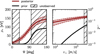 |
Fig. 12 Comparison between the priors of the inelastic mean energy loss μ∊ and the negative ionisation probability, P−, and their posterior distributions given the NILS data. |
7.2 Longer transport within the regolith grains
The mean inelastic energy loss μ∊ is larger than what is predicted by (Szabo et al. 2023b), as can be seen in Fig. 12. The amplitude A470 increased from 94.6 eV (as given by its prior in Table 1) to 147 eV (as given by its posterior in Table 3). We propose two explanations for this increase and we believe that both arguments are at play.
- (i)
The factor νE is likely smaller than unity, that is, solar wind protons are decelerated by magnetic anomalies, which would improve the agreement between the prior and posterior of μ∊. Indeed, νE and μ∊ are correlated: allowing the data to constrain νE yields νE ≈ 0.85 and A470 ≈ 110 eV. Additionally, νE may be time-dependent; if this is not accounted for, the mean inelastic energy loss could be overestimated to compensate for the increased spread in the precipitating proton energies.
- (ii)
Inelastic losses were underestimated in the simulations by Szabo et al. (2023b). This likely reflects an underestimate of the total path-length of the simulated particles in the regolith grains, rather than an underestimation of the inelastic energy loss, as the latter is well understood for hydrogen interacting with the atomic constituents of lunar regolith.
7.3 Updated sputtering and scattering yields
Our model defines a yield as the number of emitted hydrogen atoms per precipitating solar wind protons. The charge state is determined by the probability of ionisation. Regardless of the charge state of the emitted hydrogen, we find a scattering yield of  (MAP ± 68% HDI) and a sputtering yield of
  , giving a ratio of scattered to sputtered hydrogen of
  . This indicates that a proton is almost twice as likely to scatter off lunar regolith than to sputter surface hydrogen atoms.
Notably, the ENA albedo defined in Eq. (44) rises from 16% to 24%, a relatively high value compared to most previous observations (Vorburger et al. 2013). Futaana et al. (2012, Fig. 2) reported similar values, up to 30%, though their measurements were limited to the lunar equator. This increase in ηENA can be attributed to the combination of a relatively low prior probability of negative ionisation and the high fluxes measured by NILS. We note that fixing ηENA = 0.16 and sampling from the model does not change our conclusion that the probability of negative ionisation remains high.
The scattering yield for negative hydrogen ions can be estimated at first order as P−ηsc ≈ 0.15 × 0.22 = 3.3%, matching the yield of 2.5% determined by a different method reported in Wieser et al. (2025). The higher yield found here likely results from the energy distribution model of Wieser et al. (2025), which underestimates the scattered low-energy population. Similarly, the scattering yield for protons can be estimated from Lue et al. (2018), who reported a positive ionisation probability of about 5% for scattered protons of hundreds of eV. Assuming that 5% of scattered hydrogen is emitted as protons, we obtain a proton scattering yield of about 1.1%, in agreement with the values reported by Saito et al. (2008); Lue et al. (2014, 2018).
The sputtering yield for negative hydrogen ions is estimated as P−ηsp ≈ 0.10 × 0.08 = 0.8%, with the lower ionisation probability of 0.10 accounting for the lower average energy of sputtered atoms. The inferred sputtering yield, ηsp, depends on the parameter kα, which accounts for alpha-induced sputtering. If alpha particles are assumed to be about ten times more efficient at sputtering hydrogen instead of only 2.8 times as used in this paper, the inferred ηsp decreases from 8% to about 6%, with no significant change to the scattering yield ηsc or any other parameters.
Figure 13 shows a summary of the hydrogen flux through the whole system, assuming an equilibrium has been reached and the top layer of each regolith grain is saturated with hydrogen. Adding scattered and sputtered contributions together, we obtain 4.1% of the precipitating solar wind protons are emitted as negative hydrogen ions, 1.5% as positive ions and 24.4% as neutral atoms. These numbers are larger compared to previously reported values (McComas et al. 2009; Wieser et al. 2009; Schaufelberger et al. 2011; Rodríguez et al. 2012; Allegrini et al. 2013; Saul et al. 2013; Vorburger et al. 2014; Zhang et al. 2020; Saito et al. 2008; Lue et al. 2014, 2018), the values reported here differ in that they are based on a lower energy threshold of 0 eV.
The hydrogen reservoir in the top layer of each regolith grain is drained by sputtering, thermal desorption, micrometeorite impact vaporisation, sublimation and photon or electron stimulated desorption. Of these, we only model the sputtering fraction, so the observed energy spectrum (Fig. 1) could also be due to contributions from other removal processes. Including other processes would lower the reported sputtering fraction, but it is difficult to find removal process other than sputtering that result in significant fluxes up to 100 eV. This makes it likely that the reported sputtering yield is not significantly overestimated.
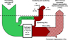 |
Fig. 13 Summary of hydrogen fluxes incident on (green) and emitted from (red) lunar regolith, assuming a solar wind speed of about 300km/s striking the surface at a 50° angle from the normal. Scattered and sputtered components are energy-integrated from 0 eV. The hydrogen reservoir represents the hydrogen-enriched top layer of regolith grains and it is assumed that the hydrogen concentration in the reservoir has reached an equilibrium. The split between permanently retained hydrogen and losses via processes such as micrometeorite vaporisation or thermal desorption remains uncertain (hatched areas). |
7.4 Angular distributions
The NILS observations cover only a limited range of emission angles. Nevertheless, for an average azimuthal emission angle of φ = 213°, the distribution of the polar emission angle β can be retrieved for both scattered and sputtered hydrogen atoms. Note that these distributions refer to emitted hydrogen atoms regardless of their charge state.
Figure 14 shows the polar emission angle distributions for forward-scattered and forward-sputtered hydrogen. The angular distribution of scattered particles is better constrained by data, as indicated by the smaller uncertainties. In contrast, the sputtering distribution is less certain, primarily due to the limited instrument coverage at low energies. For both processes, the angular emission function for β > 75° is controlled by visibility constraints. Regardless of the emission profile at the microscopic scale, the roughness of the regolith enforces a visibility reduction for near-grazing emission angles, as expressed by the dotted line in Fig. 14. At smaller β angles, the sputtered and scattered angular distributions begin to diverge.
The angular distribution of scattered particles closely matches its prior and shows little sensitivity to it, indicating that the prior provides an accurate physical description and agrees well with the data.
The angular distribution of sputtered particles rises sharply, with yields reaching up to 0.4 sr−1. The sputtering angular yield is sensitive to the width of the hierarchical scale prior, σsp, defined in Table F.1. Narrowing this prior reduces bin-to-bin variations, effectively forcing the updated sputtering angular yield towards its a priori cosine dependence (Eq. (47)). However, this worsens the agreement between the modelled and observed differential flux, particularly for emission energies between 80 eV and 200 eV.
For large polar emission angles β > 75°, our observed angular emission function differs qualitatively from the one reported in Vorburger et al. (2014) for energetic neutral hydrogen: while the former shows decreasing fluxes for large β, the latter does not show this. A possible cause for the difference is the lack of data coverage in Vorburger et al. (2014) for β close to 90°, resulting in a weakly-constrained fit.
It is important to note that, although Fig. 14 shows that the sputtering angular yields exceed the scattering angular yields at forward emission angles, the total scattering yield reported in Table 3 is higher than the total sputtering yield. This apparent discrepancy arises from the asymmetric scattering angular distribution, in which backward-scattering angles that are unobserved by NILS dominate and are constrained by the prior in Eq. (46). In contrast, the sputtering angular yield is assumed a priori to be symmetric and cannot be updated a posteriori given the limited angular coverage of NILS.
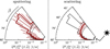 |
Fig. 14 Posterior summary of the angular yields for sputtering (left) and scattering (right) as a function of the macroscopic polar emission angle, β, at mean emission azimuth φ = 213°. In both panels, the thick red line shows the MAP estimate of the (log) angular yield in each β interval, with red radial lines indicating the 68% HDI. For comparison, the grey lines show the complementary process (scattering in the sputtering panel; sputtering in the scattering panel). Dashed red curves indicate the priors (Eqs. (46) and (47)). The dotted black curve shows the (scaled) visibility function for lunar regolith (Fig. B.1). Yields correspond to forward-scattering and forward-sputtering, as reminded by the Sun symbol. Numerical values are listed in Table F.2. |
7.5 Surface binding energy of hydrogen and other model parameters
The surface binding energy, U, of hydrogen in regolith is treated as a free parameter. Its posterior robustly converges to 4-6 eV, largely independent of the prior (within reasonable variation), with a best estimate of U = 5.5 eV. This is consistent with Kudriavtsev et al. (2005), who report 5.73 eV for hydrogen sputtered from silicon. The posterior differs only slightly from the prior, suggesting either (i) the prior is already consistent with the NILS data, and/or (ii) the data provide limited additional constraint.
The extra energy loss factor γextra in the sputtering model shrunk towards zero in the posterior. This result indicates that neglecting this factor is compatible with the NILS data.
7.6 Possible effects of lunar magnetic anomalies on the precipitating flux
The solar wind flux precipitating onto the surface is not necessarily equal to the flux measured in nearby orbit. Variations in the precipitating flux of up to a factor of 1.5 have been observed on timescales of approximately 100 s (Fig. 10). The likely cause of these variations is the proximity to magnetic anomalies, which can partially shield (Vorburger et al. 2013) or locally enhance (Wieser et al. 2010) the precipitating flux. With a single-point measurement such as NILS, temporal and spatial variations cannot be disentangled; however, it is likely that both contribute.
7.7 Limitations and caveats
Our model uses fixed values for the geometric factor of NILS without uncertainties for stability reasons. Any uncertainties in the geometric factor will directly propagate to additional uncertainties in the estimated probability of negative ionisation for hydrogen, P−. We obtained a relatively high values for P− in our analysis. Alternatively, this could be caused by a systematic underestimation of the absolute geometric factor of NILS. A careful analysis shows that an underestimation of the geometric factor by a factor of two could be possible from an instrumental point of view, but is not very likely.
A NILS internal voltage offset on the electrodes controlling the angular response of the instrument limits the angular coverage at low energies. This offset is accounted for in this study to the best of our knowledge.
The NILS data are dominated by electrons despite the electron suppression system present in the instrument. This makes the extraction of the minor negative hydrogen ion signal statistically uncertain. The differential flux of electrons increases by several orders of magnitude at low energies (Canu-Blot 2024, Fig. 6.10), further complicating the separation of the negative hydrogen ions. Although these effects have been considered in this study, small inaccuracies in the calibration of the time-of-flight (or mass) responses for electrons and hydrogen ions could propagate into large uncertainties in the mass-separation, particularly at low energies. This could explain the relatively poor agreement between the model and the observed negative hydrogen ion differential flux below 50-60 eV, as shown in Fig. 1.
8 Conclusion
We developed and validated a semi-analytical model that describes the energy and angular distributions of negative hydrogen ions scattered and sputtered from the lunar surface. The model combines a physical description of the particle transport at the surface with a macroscopic description of the near-surface environment. A key feature of the model is that it treats scattered and sputtered fluxes separately and accounts for the probability of ionisation of the emitted particles.
The model was constrained by prior information on the relevant physical processes, informed by results from other instruments, simulations, and theoretical studies. We updated these prior assumptions through Bayesian inference using the measurements obtained by the NILS instrument.
The model shows a good agreement with the NILS measurements. We observe that lunar regolith is an excellent ionising material for negative ions, with the probability of a hydrogen atom leaving the surface as a negative ion estimated at 7-20%. We also estimated that a precipitating solar wind proton has  chance of scattering and
  chance of sputtering a surface hydrogen. This result indicates that a precipitating proton is about twice as likely to scatter off lunar regolith than to sputter surface hydrogen atoms. Furthermore, we estimated that about 3.3% of the solar wind protons are scattered as negative hydrogen ions, while about 0.8% result in sputtering of a surface hydrogen atom as a negative ion.
We obtained a robust estimate of the surface binding energy, U, of hydrogen in regolith of about 5.5 eV. We obtained a large inelastic energy loss, which might reflect the fact that the total path-length of the particles in the regolith is larger than previously assumed. The surface roughness is found to control the angular emission distribution at near-specular angles for both the scattered and sputtered processes.
Our model is flexible and can be applied to other particlesurface combinations. For example, it can describe energetic neutral hydrogen atoms emitted from the lunar surface by replacing P− with P0. Data from instruments such as ASAN on Chang’e-4 offer immediate opportunities to apply this model in other contexts.
Acknowledgements
The Negative Ions on the Lunar Surface (NILS) instrument was developed by the Swedish Institute of Space Physics (IRF) in Kiruna, Sweden, on behalf of the European Space Agency (ESA). It was supported by the ESA grant No. 3-17483/22/NL/DB. Activities at NSSC were supported by the National Natural Science Foundation of China (NSFC), grant No. 42441807. NILS data is available from the European Space Agency’s Planetary Science Archive (PSA) under doi:10.57780/esa-jw5mh1u. Posterior data of the model along with the posterior of the differential fluxes are available at doi:10.5281/zenodo.19691017. For solar wind parameters we acknowledge the use of ARTEMIS-P2 (THEMIS-C) data via NASA/GSFC’s Space Physics Data Facility’s OMNIWeb (or CDAWeb) service, and OMNI data. All posterior distributions were obtained through NUTS sampling (Hoffman & Gelman 2011) implemented in the PyMC Python package (Abril-Pla et al. 2023) with a NumPyro back-end (Phan et al. 2019; Bingham et al. 2019) for JAX-based computation. Some Equations were simplified through the use of PySR, a symbolic regression Python package (Cranmer 2023).
References
- Abril-Pla, O., Andreani, V., Carroll, C., et al. 2023, PeerJ Comput. Sci., 9, e1516 [CrossRef] [Google Scholar]
- Afanas’ev, V., & Lobanova, L. 2025, Nucl. Instrum. Methods Phys. Res. B, 560, 165610 [Google Scholar]
- Allegrini, F., Dayeh, M., Desai, M., et al. 2013, Planet. Space Sci., 85, 232 [NASA ADS] [CrossRef] [Google Scholar]
- Angelopoulos, V. 2011, Space Sci. Rev., 165, 3 [Google Scholar]
- Barabash, S., Bhardwaj, A., Wieser, M., et al. 2009, Curr. Sci., 96, 526 [Google Scholar]
- Berger, M. J., Coursey, J. S., Zucker, M. A., & Chang, J. 2005, ESTAR, PSTAR, and ASTAR: Computer Programs for Calculating Stopping-Power and Range Tables for Electrons, Protons, and Helium Ions (version 1.2.3), [Online], National Institute of Standards and Technology, Gaithersburg, MD. Available: http://physics.nist.gov/Star [Accessed: 2025-11-04] [Google Scholar]
- Bertrand, J., Bertrand, P., & Ovarlez, J.-P. 2000, The Transforms and Applications Handbook, 2nd edn., ed. A. D. Poularikas (Boca Raton: CRC Press LLC) [Google Scholar]
- Bibring, J. P., Borg, J., Burlingame, A. L., et al. 1975, Lunar Planet. Sci. Conf. Proc., 3, 3471 [Google Scholar]
- Bingham, E., Chen, J. P., Jankowiak, M., et al. 2019, J. Mach. Learn. Res., 20, 28:1 [Google Scholar]
- Borisov, A. G., & Esaulov, V. A. 2000, J. Phys.: Condensed Matter, 12, R177 [Google Scholar]
- Brötzner, J., Biber, H., Szabo, P. S., et al. 2025, Commun. Earth Environ., 6 [Google Scholar]
- Brötzner, J., Kogler, M., Szabo, P. S., et al. 2026, Phys. Rev. B, 113 [Google Scholar]
- Canu-Blot, R. 2024, Negative ions in the plasma environment of the Moon : observing small signals related to plasma-surface interaction, Tech. Rep. 318, Umeå University, Department of Physics, chapter 5 (paper I) and chapter 7 (paper II) removed from the digital version [Google Scholar]
- Canu-Blot, R., Wieser, M., Kérényi, M., et al. 2025, Space Sci. Rev., 221 [Google Scholar]
- Cartry, G., Kogut, D., Achkasov, K., et al. 2017, New J. Phys., 19, 025010 [Google Scholar]
- Cassidy, T., & Johnson, R. 2005, Icarus, 176, 499 [NASA ADS] [CrossRef] [Google Scholar]
- Clark, B., Hapke, B., Pieters, C., & Britt, D. 2002, Asteroids III [Google Scholar]
- Cranmer, M. 2023, arXiv preprint [arXiv:2305.01582] [Google Scholar]
- Demkov, Y. N. 1963, Zh. Eksperim. i Teor. Fiz., 45 [Google Scholar]
- Eckstein, W. 1981, Charge Fractions of Reflected Particles (Springer Berlin Heidelberg), 157 [Google Scholar]
- Eckstein, W., & Preuss, R. 2003, J. Nucl. Mater., 320, 209 [Google Scholar]
- Estler, W. T. 1999, CIRP Ann., 48, 611 [Google Scholar]
- Falcone, G., Forlano, L., & Tolmachev, A. I. 1999, Phys. Rev. B, 60, 6352 [Google Scholar]
- Fatemi, S., Holmström, M., Futaana, Y., et al. 2014, J. Geophys. Res. Space Phys., 119, 6095 [Google Scholar]
- Fatemi, S., Lue, C., Holmström, M., et al. 2015, J. Geophys. Res.: Space Phys., 120, 4719 [Google Scholar]
- Forlano, L., Falcone, G., & Tolmachev, A. I. 1996, Il Nuovo Cimento D, 18, 873 [Google Scholar]
- Futaana, Y. 2003, J. Geophys. Res., 108, 1025 [Google Scholar]
- Futaana, Y., Barabash, S., Wieser, M., et al. 2012, J. Geophys. Res.: Planets, 117 [Google Scholar]
- Futaana, Y., Barabash, S., Wieser, M., et al. 2013, Geophys. Res. Lett., 40, 262 [NASA ADS] [CrossRef] [Google Scholar]
- Gainullin, I. K. 2020, Phys. Usp., 63, 888 [Google Scholar]
- Gelman, A. 2014, Bayesian Data Analysis, 3rd edn., eds. J. B. Carlin, H. S. Stern, D. B. Dunson, A. Vehtari, & D. B. Rubin, A. Chapman & Hall book (Boca Raton: CRC Press, Taylor & Francis Group), 607 [Google Scholar]
- Gelman, A., & Rubin, D. B. 1992, Statist. Sci., 7 [Google Scholar]
- Halekas, J. S., Brain, D. A., Lin, R. P., & Mitchell, D. L. 2008, Adv. Space Res., 41, 1319 [Google Scholar]
- Halekas, J. S., Poppe, A. R., McFadden, J. P., et al. 2014, Geophys. Res. Lett., 41, 7436 [Google Scholar]
- Halekas, J. S., Poppe, A. R., Lue, C., Farrell, W. M., & McFadden, J. P. 2017, J. Geophys. Res.: Space Phys., 122, 6240 [Google Scholar]
- Heiken, G. 1975, Rev. Geophys., 13, 567 [Google Scholar]
- Helfenstein, P., & Shepard, M. K. 1999, Icarus, 141, 107 [Google Scholar]
- Hoffman, M. D., & Gelman, A. 2011, arXiv preprint [arXiv:1111.4246] [Google Scholar]
- Jamnig, A. 2020, Theses, Université de Poitiers, Université de Linköping (Suède) [Google Scholar]
- Jans, S., Wurz, P., Schletti, R., et al. 2001, Nucl. Instrum. Methods B, 173, 503 [Google Scholar]
- Jeffreys, H. 1946, Proc. Roy. Soc. Lond. A Math. Phys. Sci., 186, 453 [Google Scholar]
- Jäggi, N., Biber, H., Brötzner, J., et al. 2024, Planet. Sci. J., 5, 75 [Google Scholar]
- Kaneko, T. 1990, Surf. Sci., 236, 203 [Google Scholar]
- Kawano, H., & Page, F. M. 1983, Int. J. Mass Spectrom. Ion Phys., 50, 1 [Google Scholar]
- Kenmotsu, T., Yamamura, Y., Ono, T., & Kawamura, T. 2004, J. Plasma Fusion Res., 80, 406 [CrossRef] [Google Scholar]
- King, J. H., & Papitashvili, N. E. 2005, J. Geophys. Res.: Space Phys., 110 [Google Scholar]
- Kruschke, J. K. 2021, Nat. Hum. Behav., 5, 1282 [Google Scholar]
- Kudriavtsev, Y., Villegas, A., Godines, A., & Asomoza, R. 2005, Appl. Surf. Sci., 239, 273 [CrossRef] [Google Scholar]
- Lang, N. D., & Nørskov, J. K. 1983, Phys. Scr., T6, 15 [Google Scholar]
- Li, C., Hu, H., Yang, M.-F., et al. 2024, Natl. Sci. Rev., 11 [Google Scholar]
- Lienemann, J., Blauth, D., Wethekam, S., et al. 2011, Nucl. Instrum. Methods Phys. Res. B, 269, 915 [Google Scholar]
- Lin, H., Chang, R., Xu, R., et al. 2025, Nat. Geosci., 18, 1097 [Google Scholar]
- Lindhard, J., & Scharff, M. 1961, Phys. Rev., 124, 128 [Google Scholar]
- Lindhard, J., Nielsen, V., & Scharff, M. 1968, Kgl. Dan. Vidensk. Selsk., Mat.-Fys. Medd., 36 [Google Scholar]
- Littmark, U., & Gras-Marti, A. 1978, Appl. Phys., 16, 247 [Google Scholar]
- Liu, B., Zeng, X., Xu, R., et al. 2025, Nat. Astron., 9, 1776 [Google Scholar]
- Los, J., & Geerlings, J. 1990, Phys. Rep., 190, 133 [Google Scholar]
- Lue, C., Futaana, Y., Barabash, S., et al. 2011, Geophys. Res. Lett., 38 [Google Scholar]
- Lue, C., Futaana, Y., Barabash, S., et al. 2014, J. Geophys. Res.: Planets, 119, 968 [Google Scholar]
- Lue, C., Futaana, Y., Barabash, S., et al. 2016, J. Geophys. Res.: Space Phys., 121, 432 [Google Scholar]
- Lue, C., Halekas, J. S., Poppe, A. R., & McFadden, J. P. 2018, J. Geophys. Res.: Space Phys., 123, 5289 [Google Scholar]
- Maazouz, M., Guillemot, L., Esaulov, V., & O’Connor, D. 1998, Surf. Sci., 398, 49 [Google Scholar]
- Maynadié, T., Futaana, Y., Barabash, S., et al. 2025, J. Geophys. Res.: Space Phys., 130 [Google Scholar]
- McComas, D. J., Allegrini, F., Bochsler, P., et al. 2009, Geophys. Res. Lett., 36 [Google Scholar]
- McFadden, J. P., Carlson, C. W., Larson, D., et al. 2008, Space Sci. Rev., 141, 277 [Google Scholar]
- Meyer, F. W., Harris, P. R., Taylor, C. N., et al. 2011, Nucl. Instrum. Methods Phys. Res. B, 269, 1316 [Google Scholar]
- Morrissey, L. S., Bringuier, S., Bu, C., et al. 2024, Planet. Sci. J., 5, 272 [Google Scholar]
- Niehus, H., Heiland, W., & Taglauer, E. 1993, Surf. Sci. Rep., 17, 213 [Google Scholar]
- Ono, T., Aoki, Y., Kawamura, T., Kenmotsu, T., & Yamamura, Y. 2005, J. Nucl. Mater., 337-339, 975 [Google Scholar]
- Papaspiliopoulos, O., Roberts, G. O., & Sköld, M. 2007, Statist. Sci., 22 [Google Scholar]
- Papike, J. J., Simon, S. B., & Laul, J. C. 1982, Rev. Geophys., 20, 761 [Google Scholar]
- Pešić, Z. D., Vikor, G., Atanassova, S., et al. 2007, Phys. Rev. A, 75, 012903 [Google Scholar]
- Phan, D., Pradhan, N., & Jankowiak, M. 2019, arXiv preprint [arXiv:1912.11554] [Google Scholar]
- Pieters, C. M., & Noble, S. K. 2016, J. Geophys. Res.: Planets, 121, 1865 [NASA ADS] [CrossRef] [Google Scholar]
- Raue, A., Kreutz, C., Maiwald, T., et al. 2009, Bioinformatics, 25, 1923 [CrossRef] [PubMed] [Google Scholar]
- Rodríguez M. D., Saul, L., Wurz, P., et al. 2012, Planet. Space Sci., 60, 297 [NASA ADS] [CrossRef] [Google Scholar]
- Saito, Y., Yokota, S., Tanaka, T., et al. 2008, Geophys. Res. Lett., 35 [Google Scholar]
- Saito, Y., Nishino, M. N., Fujimoto, M., et al. 2012, Earth Planets Space, 64, 83 [Google Scholar]
- Saul, L., Wurz, P., Vorburger, A., et al. 2013, Planet. Space Sci., 84, 1 [NASA ADS] [CrossRef] [Google Scholar]
- Schaufelberger, A., Wurz, P., Barabash, S., et al. 2011, Geophys. Res. Lett., 38 [Google Scholar]
- Schenkel, T., Briere, M. A., Schmidt-Böcking, H., Bethge, K., & Schneider, D. H. 1997, Phys. Rev. Lett., 78, 2481 [Google Scholar]
- Sigmund, P. 1969, Phys. Rev., 184, 383 [CrossRef] [Google Scholar]
- Sukhomlinov, V. S. 1997, Tech. Phys., 42, 14 [Google Scholar]
- Szabo, P., Cupak, C., Biber, H., et al. 2022, Surf. Interfaces, 30, 101924 [Google Scholar]
- Szabo, P. S., Poppe, A., Mutzke, A., et al. 2023a, Energetic Neutral Atom (ENA) emission characteristics at the Moon and Mercury from 3D regolith simulations of solar wind reflection (Dataset) [Google Scholar]
- Szabo, P. S., Poppe, A. R., Mutzke, A., et al. 2023b, J. Geophys. Res.: Planets, 128 [Google Scholar]
- Tanaka, T., Saito, Y., Yokota, S., et al. 2009, Geophys. Res. Lett., 36 [Google Scholar]
- Thompson, M. W., Farmery, B. W., & Newson, P. A. 1968, Philos. Mag., 18, 361 [Google Scholar]
- Tolmachev, A. 1999, Nucl. Instrum. Methods Phys. Res. B, 155, 36 [Google Scholar]
- Tucker, O. J., Farrell, W. M., Killen, R. M., & Hurley, D. M. 2019, J. Geophys. Res.: Planets, 124, 278 [Google Scholar]
- Verbeek, H., Eckstein, W., & Bhattacharya, R. 1980, Surf. Sci., 95, 380 [Google Scholar]
- von Toussaint, U., Mutzke, A., & Manhard, A. 2017, Phys. Scr., 2017, 014056 [Google Scholar]
- Vorburger, A., Wurz, P., Barabash, S., et al. 2012, J. Geophys. Res., 117 [Google Scholar]
- Vorburger, A., Wurz, P., Barabash, S., et al. 2013, J. Geophys. Res.: Space Phys., 118, 3937 [Google Scholar]
- Vorburger, A., Wurz, P., Barabash, S., et al. 2014, J. Geophys. Res.: Space Phys., 119, 709 [Google Scholar]
- Wang, N. P., García, E. A., Monreal, R., et al. 2001, Phys. Rev. A, 64, 012901 [Google Scholar]
- Watanabe, S. 2010, J. Mach. Learn. Res., 11, 3571 [Google Scholar]
- Wieser, M., Wurz, P., Brüning, K., & Heiland, W. 2002, Nucl. Instrum. Methods Phys. Res. B, 192, 370 [Google Scholar]
- Wieser, M., Barabash, S., Futaana, Y., et al. 2009, Planet. Space Sci., 57, 2132 [NASA ADS] [CrossRef] [Google Scholar]
- Wieser, M., Barabash, S., Futaana, Y., et al. 2010, Geophys. Res. Lett., 37 [Google Scholar]
- Wieser, M., Barabash, S., Wang, X.-D., et al. 2020, Space Sci. Rev., 216, 73 [CrossRef] [Google Scholar]
- Wieser, M., Williamson, H., Wieser, G. S., et al. 2024, A&A, 684, A146 [NASA ADS] [CrossRef] [EDP Sciences] [Google Scholar]
- Wieser, M., Zhang, A., Canu-Blot, R., et al. 2025, Commun. Earth Environ., 6 [Google Scholar]
- Wilson, W. D., Haggmark, L. G., & Biersack, J. P. 1977, Phys. Rev. B, 15, 2458 [CrossRef] [Google Scholar]
- Wucher, A. 2008, Appl. Surf. Sci., 255, 1194 [Google Scholar]
- Wucher, A., Weidtmann, B., & Duvenbeck, A. 2013, Nucl. Instrum. Methods Phys. Res. B, 303, 108 [Google Scholar]
- Wurz, P., Scheer, J., & Wieser, M. 2006, e-J. Surf. Sci. Nanotechnol., 4, 394 [Google Scholar]
- Wurz, P., Fatemi, S., Galli, A., et al. 2022, Space Sci. Rev., 218 [Google Scholar]
- Yokota, S., Saito, Y., Asamura, K., et al. 2009, Geophys. Res. Lett., 36 [Google Scholar]
- Zeng, X., Liu, D., Chen, Y., et al. 2023, Nat. Astron., 7, 1188 [Google Scholar]
- Zhang, A., Wieser, M., Wang, C., et al. 2020, Planet. Space Sci., 189, 104970 [Google Scholar]
- Zhang, H., Li, C., You, J., et al. 2022, Aerospace, 9, 358 [NASA ADS] [CrossRef] [Google Scholar]
- Zhou, C., Tang, H., Li, X., et al. 2022, Nat. Commun., 13, 5336 [Google Scholar]
- Ziegler, J. F., & Biersack, J. P. 1985, The Stopping and Range of Ions in Matter (Springer US), 93 [Google Scholar]
Appendix A Inference summary
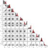 |
Fig. A.1 Pair-plot of the joint posterior distribution |

Appendix B Regolith as a rough surface
B.1 Microscopic polar emission angle
Szabo et al. (2022) present a statistical model for the distribution of inclination angles of a random Gaussian rough surface, characterised by a single roughness parameter, w. From this parameter, the mean surface inclination can be derived as (Szabo et al. 2022, Eq. 4)
![Mathematical equation: \delta_m \;\left[\mathrm{rad}\right] \equiv \dfrac{\pi}{2} \exp\left[\frac{1}{2w^2}\right] \mathtt{erfc}\left[\frac{1}{w\sqrt{2}}\right]\;,](/articles/aa/full_html/2026/06/aa59499-26/aa59499-26-eq119.png) (B.1)
(B.1)
where erfc denotes the complementary error function. Brötzner et al. (2025) estimated the mean inclination angle of an Apollo 16 regolith sample to be δm = 27.7°. Helfenstein & Shepard (1999) report larger mean slopes of approximately 40° at the 0.1 mm scale, but with a significant uncertainty of about 20° (1σ). For this reason, we use the first estimate δm = 27.7° to describe the roughness of the lunar surface observed by NILS, and solve Eq. B.1 for w, obtaining w ≈ 0.45. However, we note that Brötzner et al. (2025) studied pressed regolith pellets, which may have altered the overall roughness.
We construct a mapping between the macroscopic polar emission angle β and the microscopic angle β′ using Szabo et al. (2022, Eq. C4):
 (B.2)
(B.2)
where (p, q) are the surface slopes (Szabo et al. 2022, see Fig. A1), and φ′ is the microscopic azimuthal emission angle. To obtain β′ from this relation, we sample (p, q) from the joint normal distribution (p, q) ∼ N(0, w2) (Szabo et al. 2022, Eq. A2), and uniformly sample the macroscopic and microscopic angles: φ′ ∼ Uniform(0,2π) and cos β ∼ Uniform(0,1). The resulting mapping is shown in Fig. B.1, with Eq. 9 drawn as a thick red line.
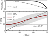 |
Fig. B.1 Mapping between the macroscopic polar emission angle β and the microscopic polar emission angle β′ for a rough surface of mean inclination angle of δm = 27.7° (dotted line). The thick red line shows the average β′ for any β, along with a 68% percentile range (gray shaded region) and the unity line (dashed line). |
B.2 Shadowing
In the case of rough surfaces, a particle that leaves the surface may be redeposited on its way out. We describe the probability that a particle, leaving the surface at a macroscopic emission polar angle β, impacts the surface again and is therefore unobserved by the instrument as the visibility probability S, defined as (Szabo et al. 2022, Eq. 9, 13, C5):
 (B.3a)
 (B.3b)
The visibility probability is given for w = 0.45 in Fig. B.1.
Appendix C Instrument model
The instrument reports a number of counts C per measurement time τ. This section describes the conversion between the count rate C/τ and the differential number flux J.
The instrument scans the phase-space incrementally. We label each observation of the phase-space by a velocity vector u, as defined in Canu-Blot et al. (2025, Eq. 5). From Canu-Blot et al. (2025, Eq. 55 and 58), we write
 (C.1)
(C.1)
where A [cm2] is the effective area of the instrument, GF0 [cm sr eV/eV] is the absolute geometric factor of the instrument (Canu-Blot et al. 2025, Eq. 73), κ [sr eV/q] is a scaling factor (Canu-Blot et al. 2025, Eq. 10), η is the detection probability (Canu-Blot et al. 2025, Sect. 4.7.2), and (ξu, ωu) are the average energy-per-charge [eV/q] and elevation of a measurement u, respectively. The elevation angle is historically noted θ but to avoid conflicting notation, we name it ω. The approximation in Eq. C.1 comes from the following simplification (with an average error of 1% over the instrument coverage)
 (C.2)
(C.2)
where Rω [1/sr] is the angular response of the instrument and α the azimuthal angle.
We replace A(u) κ (u) in Canu-Blot et al. (2025, Eq. 57) by the approximation of Eq. C.1, make the assumption that the differential flux does not posses any structure smaller than the energy response of the instrument, and note that J = 2Ef/m, with f the phase-space density of a species of mass m, and we obtain
 (C.3a)
 (C.3b)
We now make the assumption that the differential flux varies little over the azimuthal coverage of the angular response of the instrument. This gives
 (C.4a)
 (C.4b)
The integral in Eq. C.4 is defined in the instrument frame (see Canu-Blot et al. (2025, Sect. 4.1.3) for more details), and we now express it using the emission angles (β, φ) (see Fig. 2) using the transformation defined in Wieser et al. (2025, Eqs. 14, 15, and 16).
 (C.5)
(C.5)
with φu = f2 (ωu, αu; SAA), where f2 is defined in Wieser et al. (2025, Eq. 13) and αu = –0.752° (Canu-Blot et al. 2025, Eq. 16). We neglect the dependency over ω, and approximate  , where SAA ≈ 34° is the average SAA over the mission.
Appendix D Bayesian inference
The NILS dataset consists of 302 minutes of observations, with the instrument viewing the lunar surface for about half of that time. The near-surface environment is dominated by secondary electrons, photoelectrons, and UV radiation, all of which complicate the study of the weaker negative ion signal. We use Bayesian inference to extract and study the signal.
We first define the set of observed counts as C, that is, the number of counts observed in the time-energy-angular-mass matrix. We assume that the observed counts are drawn from a Poisson (Pois) distribution such that
 (D.1)
(D.1)
where ![Mathematical equation: $\vec{\Lambda} \equiv \left[\lambda_{\mathrm{H}^-}, \vec{\lambda_\mathrm{nuis}}\right]$](/articles/aa/full_html/2026/06/aa59499-26/aa59499-26-eq132.png) , with λH- the rate of negative hydrogen ions and λnuis the contribution of all other nuisance signals-namely, electrons, oxygen ions and UV. The matrix F defines the mass response of the instrument, as given by Canu-Blot et al. (2025, Sect. 4.6). The matrix Λ thus defines the signal rates over the time-energy-angular space.
, with λH- the rate of negative hydrogen ions and λnuis the contribution of all other nuisance signals-namely, electrons, oxygen ions and UV. The matrix F defines the mass response of the instrument, as given by Canu-Blot et al. (2025, Sect. 4.6). The matrix Λ thus defines the signal rates over the time-energy-angular space.
We wish to infer knowledge about the negative hydrogen ion differential flux J−H. We link the rate λH− with J−H using the instrument response defined by Eq. C.5. We thereafter simplify the notation by introducing λ ≡ λH− and J ≡ J−H, and obtain the deterministic relation
![Mathematical equation: \mathbb{P}\left(\lambda \mid \mathcal{J}\right) = \delta\left[\lambda - \lambda_{\mathrm{model}}\left(\mathcal{J}\right)\right]\;,](/articles/aa/full_html/2026/06/aa59499-26/aa59499-26-eq133.png) (D.2)
(D.2)
where the relation λmodel (J) is defined by Eq. C.5. We introduce the statistical distribution of the differential flux conditional on the observed data (thereafter called posterior distribution), P (J | C). We apply Bayes’ theorem and express the probability distribution in proportional form by omitting the marginal likelihood
 (D.3)
(D.3)
We introduce the rate matrix Λ and the mass response of the instrument F into P (C | J), giving:
 (D.4)
(D.4)
From the assumptions that (i) λ and λnuis are mutually independent; (ii) F and λnuis do not depend on J; (iii) the uncertainty in the mass response of the instrument can be neglected, we obtain
 (D.5)
(D.5)
From Eqs. D.1 and D.2, and integrating over λ, we obtain
![Mathematical equation: \mathbb{P}\left(\mathcal{J}\mid\vec{\mathcal{C}}\right) \propto \mathbb{P}\left(\mathcal{J}\right) \!\!\int \mathtt{Pois}\left(\left[\lambda_\mathrm{model}\left(\mathcal{J}\right), \vec{\lambda_\mathrm{nuis}}\right] \cdot \vec{\mathrm{F}}\right) \mathbb{P}\left(\vec{\lambda_\mathrm{nuis}}\right) \mathrm{d}\vec{\lambda_\mathrm{nuis}}.](/articles/aa/full_html/2026/06/aa59499-26/aa59499-26-eq137.png) (D.6)
(D.6)
We used a Jeffreys prior (Jeffreys 1946) on P (λnuis). This non-informative prior is invariant under re-parametrisation, providing an objective baseline when prior knowledge is limited. The prior P (J | C) is described through the priors in Sect. 5.1, the Table F.1, and the model in Eq. 42.
Appendix E Normalisation of scattering energy model
The model for the energy distribution of scattered particles is computationally expensive, especially with respect to Eq. 33, which evaluates the function  N-times to marginalise it over the inelastic energy loss. Below, we give an alternative definition of the normalisation factor, n, obtained from the non-dimensionalisation of the distribution,
  .
.
E.1 Non-dimensionalisation
We reduce the dimensionality of the problem by normalising over the incident energy, Ein. We introduce the dimensionless variables
 (E.1a)
 (E.1b)
 (E.1c)
 (E.1d)
 (E.1e)
We obtain the energy distribution in reduced form
 (E.2)
(E.2)
with x and f defined as in Eq. 26. Noting that
 (E.3a)
 (E.3b)
we can write the normalisation factor,  , independent of Ein, as
![Mathematical equation: \mathtt{n}\left(u,\Delta_\epsilon'\right) = 2 \int_0^{\,\kappa\ln \left(A/u\right)} \left[1-\dfrac{u}{A}\exp\left(x/\kappa\right)\right]f\left(x\right)\mathrm{d}x\;.](/articles/aa/full_html/2026/06/aa59499-26/aa59499-26-eq149.png) (E.4)
(E.4)
E.2 Analytical approximation
For the special case of (p = 0.97, κ = 7.3), corresponding to a proton impacting lunar regolith at 300 km/s, that is MP = 1 amu, MS = 21.9amu, and m = 0.57, we approximate the function n (u, Δ′∊) by
 (E.5)
(E.5)
The approximation is valid for Δ′∊ ∊ [1 × 10−3,0.95] and u ∊ [1 × 10⁻³, 2 × 10⁻²], which covers most of the possible surface binding energies, inelastic losses, and solar wind energies. Within this space, the approximation has a mean relative error of 0.4%, and loses accuracy (relative error of about 10%) for large Δ′∊ > 0.9.
Appendix F Extra content
F.1 Definition of priors
We define here all prior distributions not mentioned in Sect. 5.1.
Definition of prior knowledge
The dependence of the scattering angular emission distribution  and the sputtering angular emission distribution
  over the macroscopic emission polar angle βi is discretised in 11 linearly-spaced angular intervals, indexed i = 1,..., 11. We used a hierarchical, non-centred log-normal parametrisation defined as (e.g. for the sputtered process), expressed as
![Mathematical equation: \mathcal{J}_{\Omega}^\mathrm{sp}\left(\beta_i,\overline{\phi}\right) = \exp\left[\ln\left[\mathcal{J}_{\Omega}^\mathrm{sp, \, prior}\left(\beta_i,\overline{\phi}\right)\right] + \sigma^\mathrm{sp} \times \epsilon_i^\mathrm{sp}\right]\;.](/articles/aa/full_html/2026/06/aa59499-26/aa59499-26-eq157.png) (F.1)
(F.1)
The choice of a hierarchical parametrisation allows for smooth and weakly informative variation across angular bins, while a non-centred parametrisation reduces the correlation between the per-bin angular yield and the scale parameter σsp and σsc(Papaspiliopoulos et al. 2007).
We systematically verified the choice of priors through predictive prior modelling. We studied heuristically the sensitivity of the inference on the choice of priors. In all cases, the main conclusions of this study remained robust to reasonable variations in the prior assumptions.
F.2 Posterior summary of angular yields
Table F.2 summarises the marginal posterior distributions of the scattering and sputtering angular yields.
Marginal posterior distributions for the sputtering and scattering angular yields.
All Tables
Marginal posterior distributions for the sputtering and scattering angular yields.
All Figures
|
Fig. 1 Differential number flux of negative hydrogen ions, J−H, versus emission energy. Vertical bars show flux estimates, with thick and thin bars representing the 68% and 90% highest density intervals, respectively. Bar colour qualitatively reflects signal significance, based on the Widely Applicable Information Criterion (Watanabe 2010) which estimates out-of-sample predictive accuracy, by comparing models with and without hydrogen. Each panel corresponds to a specific emission polar angle interval β (shown in the upper-right inset), where inward arrows indicate the average SZA. The energy-axis arrow marks the average undisturbed solar wind proton energy. Hatched regions indicate energies without data coverage. Lines show the median modelled flux of scattered (black dashed), sputtered (black dash-dotted), and total (solid red) negative hydrogen ions; the gray shading denotes the 68% highest density interval of the total modelled flux. |
| In the text | |
|
Fig. 2 Illustration of the solar wind impinging angles (orange) and emission angles (blue). An arbitrary angular emission profile is drawn, with dashed arrows representing possible emission directions. Both the SZA and the emission polar angle, β, are defined relative to the surface normal. The SAA is relative to the northerly direction, and the emission azimuthal angle, φ, is relative to the SAA. The total scattering angle Ψ is the angle between the solar wind direction and the emission direction. |
| In the text | |
|
Fig. 3 Probability of negative ionisation as a function of the perpendicular emission velocity, v⊥, for 1 keV (≈4.37 × 10⁵ m/s) hydrogen ions scattering off silicon. The mapping to the emission energy for different microscopic emission angles, β′ (Section 4.5) is shown below the figure. Data points (open circles) are taken from Maazouz et al. (1998, Fig. 5a), with the best fit from Eq. (7) shown as a dashed line and that from Eq. (8) shown as a solid line. |
| In the text | |
|
Fig. 4 Schematised sputtering induced by light ions. A proton (filled red circle) directed towards the surface: (1) rapidly neutralises to an hydrogen atom (open circle); (2) penetrates the material and loses a fraction γextra of its energy; (3) undergoes a large-angle scattering on a surface atom (filled black circles); (4) creates an isotropic emission of hydrogen primary knock-on atoms (PKAs, open circles) while losing additional energy inelastically (yellow overlay); most knock-on hydrogen atoms do not escape the surface (crosses) while those near the surface (5) have an increased probability of escaping the surface; (6) charge-exchange transfers (green arrows) may ultimately lead to a negative charge state (filled blue circle). |
| In the text | |
|
Fig. 5 Energy distribution of hydrogen atoms sputtered by 300 km/s solar wind H+ and He++ ions impacting the lunar regolith (the energies of the projectiles are marked by an upward arrow). All curves are computed with a surface binding energy for hydrogen of U = 5 eV, except for the thin red lines, which illustrate the effect of varying U on the energy distribution. Four models are shown: proton-induced sputtering without extra energy loss (solid black line); proton-induced sputtering with extra energy loss (dashed black line); sputtering from both protons and alpha particles, assuming an alpha-to-proton ratio of 4% and no extra energy loss (red solid line, with the thin red lines the same model computed for U = 1 eV and 10 eV); and the modified SigmundThompson model as defined by Wurz et al. (2022, Eq. (25)) calculated for a proton-induced sputtering of hydrogen. |
| In the text | |
|
Fig. 6 Schematised scattering of light ions from a surface. A proton (red filled circle) directed towards the surface: (1) rapidly neutralises; (2) scatter at small-to-medium angles off at least two surface atoms (black filled circles); (3) loses energy inelastically (yellow overlay); (4) exits the surface while charge-exchange transfers (green arrows) may lead to a final negative charge state (blue filled circle). |
| In the text | |
|
Fig. 7 Comparison of our energy distribution model with simulation data for 300 km/s solar wind protons (470 eV) scattering off lunar regolith at three different scattering angles. Panels a-c show the fitted model for three different total scattering angles Φ = 60°, 100°, and 160°, respectively. The original model from Forlano et al. (1996) in panel a provides a reasonable match to the simulation data but generally overestimates the energy loss. The energy straggling is set to σ∊ = 0.7 μ∊. For both panels b and c: the original model (dotted line) from Forlano et al. (1996) provides a reasonable average fit but consistently overestimates the energy of the high-energy scattered population. The modified model (Eq. (26); dash-dotted line), which includes a constant inelastic loss, improves the fit, though it underestimates the width of the high-energy peak at large scattering angles. Including energy loss straggling (Eq. (34), red solid line) further improves the fit. All comparisons use a surface binding energy of U = 5 eV. Note that in panel a) only one line (dotted) is shown as all three models coincide. |
| In the text | |
|
Fig. 8 Relation between the mean inelastic energy loss, μ∊, and the total scattering angle, Ψ. The mean inelastic energy loss is fitted for different SZA values (crosses: normal incidence; circles: 60° incidence) and for various emission angles. Crosses are shifted by −5° for clarity. Equation (39) is shown as the solid red line. The fits from the three panels in Fig. 7 are labelled. |
| In the text | |
|
Fig. 9 Comparison between the energy distribution model (Eq. (34) solid lines) and simulated energy distributions (open circles) of solar wind proton scattering at normal incidence on the lunar regolith for proton incident speeds of 300 km/s (blue) and 500 km/s (red) (Szabo et al. 2023b, Figs. 4 and 5). The thick lines show models computed with a surface binding energy of U = 5 eV. Varying U primarily affects the low-energy tail of the distribution, as illustrated by the thin blue lines, which span U = 1-10 eV. |
| In the text | |
|
Fig. 10 Energy-time spectrogram of the negative hydrogen ions energy-differential flux at the surface, normalised by the upstream solar wind flux. The flux is expressed in units of 1/sr. The flux is averaged over angles. The time is discontinuous with each bin labelled by its average date (UTC). Upper panel: temporal variation of the solar wind flux enhancement and reduction factor, νf, with the red horizontal line the best estimate (at the maximum a posteriori) and the vertical error bars the uncertainty (68% highest density interval). Lower panel: the red solid line represents the upstream energy. Increases in the observed normalised flux are well reproduced by the model, corresponding to increases in the factor vf. |
| In the text | |
|
Fig. 11 Lunar topography and observed macroscopic polar emission angle near the Chang’e-6 landing site (Liu et al. 2025). Panel a: elevation relative to the lander. The estimated blast radius of the retro rockets of the lander is indicated by the white dashed line. Panel b: observed emission angle β. Regions that are occulted and not visible from NILS due to local surface topography are shown in black. In both panels, black contours indicate the sensitivity level of the instrument projected onto the surface: 20% (solid line); 50% (dashed line) and 90% (dotted line). North is directed upwards. |
| In the text | |
|
Fig. 12 Comparison between the priors of the inelastic mean energy loss μ∊ and the negative ionisation probability, P−, and their posterior distributions given the NILS data. |
| In the text | |
|
Fig. 13 Summary of hydrogen fluxes incident on (green) and emitted from (red) lunar regolith, assuming a solar wind speed of about 300km/s striking the surface at a 50° angle from the normal. Scattered and sputtered components are energy-integrated from 0 eV. The hydrogen reservoir represents the hydrogen-enriched top layer of regolith grains and it is assumed that the hydrogen concentration in the reservoir has reached an equilibrium. The split between permanently retained hydrogen and losses via processes such as micrometeorite vaporisation or thermal desorption remains uncertain (hatched areas). |
| In the text | |
|
Fig. 14 Posterior summary of the angular yields for sputtering (left) and scattering (right) as a function of the macroscopic polar emission angle, β, at mean emission azimuth φ = 213°. In both panels, the thick red line shows the MAP estimate of the (log) angular yield in each β interval, with red radial lines indicating the 68% HDI. For comparison, the grey lines show the complementary process (scattering in the sputtering panel; sputtering in the scattering panel). Dashed red curves indicate the priors (Eqs. (46) and (47)). The dotted black curve shows the (scaled) visibility function for lunar regolith (Fig. B.1). Yields correspond to forward-scattering and forward-sputtering, as reminded by the Sun symbol. Numerical values are listed in Table F.2. |
| In the text | |
|
Fig. A.1 Pair-plot of the joint posterior distribution |
| In the text | |
|
Fig. B.1 Mapping between the macroscopic polar emission angle β and the microscopic polar emission angle β′ for a rough surface of mean inclination angle of δm = 27.7° (dotted line). The thick red line shows the average β′ for any β, along with a 68% percentile range (gray shaded region) and the unity line (dashed line). |
| In the text | |
Current usage metrics show cumulative count of Article Views (full-text article views including HTML views, PDF and ePub downloads, according to the available data) and Abstracts Views on Vision4Press platform.
Data correspond to usage on the plateform after 2015. The current usage metrics is available 48-96 hours after online publication and is updated daily on week days.
Initial download of the metrics may take a while.