| Issue |
A&A
Volume 684, April 2024
|
|
|---|---|---|
| Article Number | A146 | |
| Number of page(s) | 6 | |
| Section | Planets and planetary systems | |
| DOI | https://doi.org/10.1051/0004-6361/202348876 | |
| Published online | 16 April 2024 | |
Energy spectra of energetic neutral hydrogen backscattered and sputtered from the lunar regolith by the solar wind★
1
Swedish Institute of Space Physics,
Kiruna, Sweden
e-mail: This email address is being protected from spambots. You need JavaScript enabled to view it.
2
National Space Science Center, Chinese Academy of Sciences,
Beijing, PR China
3
University of Chinese Academy of Sciences,
Beijing, PR China
Received:
7
December
2023
Accepted:
6
February
2024
Abstract
Context. The solar wind impinging on the lunar surface results in the emission of energetic neutral atoms. This particle population is one of the sources of the lunar exosphere.
Aims. We present a semi-empirical model to describe the energy spectra of the neutral emitted atoms.
Methods. We used data from the Advanced Small Analyzer for Neutrals (ASAN) on board the Yutu-2 rover of the Chang’E-4 mission to calculate high-resolution average energy spectra of the energetic neutral hydrogen flux from the surface. We then constructed a semi-empirical model to describe these spectra.
Results. Excellent agreement between the model and the observed energetic neutral hydrogen data was achieved. The model is also suitable for describing heavier neutral species emitted from the surface.
Conclusions. A semi-analytical model describing the energy spectrum of energetic neutral atoms emitted from the lunar surface has been developed and validated by data obtained from the lunar surface.
Key words: plasmas / scattering / Moon / planets and satellites: surfaces
The ASAN data used in this study is available though the Data Release and Information Service System of China’s Lunar Exploration Program (https://moon.bao.ac.cn/ce5web/moonGisMap.search and https://moon.bao.ac.cn/ce5web/searchOrder_hyperSearchData.search?pid=CE4/ASAN) or through a reasonable request from the authors. We acknowledge use of NASA/GSFC’s Space Physics Data Facility’s OMNIWeb (or CDAWeb) service, and OMNI data.
© The Authors 2024
 Open Access article, published by EDP Sciences, under the terms of the Creative Commons Attribution License (https://creativecommons.org/licenses/by/4.0), which permits unrestricted use, distribution, and reproduction in any medium, provided the original work is properly cited.
This article is published in open access under the Subscribe to Open model. This email address is being protected from spambots. You need JavaScript enabled to view it. to support open access publication.
1 Introduction
The lunar surface, composed of mainly silicate minerals, has undergone extensive space weathering, creating a thick regolith layer. As the moon is lacking an atmosphere and an intrinsic global magnetic field, solar wind ions are able to directly interact with the surface regolith. In the Apollo era, the solar wind was thought to be almost completely absorbed by the lunar surface (Berisch & Wittmaack 1991; Feldman et al. 2000; Crider & Vondrak 2002).
However, measurements of energetic neutral atoms by the Chandrayaan-1 mission (Goswami & Annadurai 2009; Barabash et al. 2009) and the Interstellar Boundary Explorer (IBEX) McComas et al. (2009) showed that a large fraction, up to 20%, of solar wind protons are directly reflected back from the regolith to space as energetic neutral hydrogen atoms (Wieser et al. 2009; Funsten et al. 2013; Allegrini et al. 2013). These particles are one of the sources of the lunar exosphere, together with particles sputtered from the lunar regolith by the solar wind, materials vaporised by impacting micrometeorites and outgassing from the lunar mantle. The angular and energy distributions of backscattered and sputtered particles can give an insight into the microphysics of the scattering and sputtering processes themselves.
Futaana et al. (2012) found that the energy distribution of energetic neutral hydrogen atoms detected by Chandrayaan-1 was well fitted by a Maxwell-Boltzmann distribution instead of the expected Thompson-Sigmund spectrum. The reason for this is that the Thompson-Sigmund law only describes the sputtered component and not the backscattered solar wind. The temperature of the Maxwell-Boltzmann distribution strongly correlated with the solar wind velocity.
Futaana et al. (2012) subsequently calculated a backscatter-ing fraction for the solar wind of ~0.19, which is independent of upstream solar wind parameters. Analysis of the angular distribution of the emitted energetic neutral hydrogen showed a preference for scattering in the backward direction over forward scattering relative to the direction of the solar wind impinging on the surface. This was attributed to the porosity of the lunar regolith (Schaufelberger et al. 2011).
Data from the IBEX instruments showed an energetic neutral atom albedo of 0.08–0.2 (Funsten et al. 2013; Rodriguez et al. 2012; Saul et al. 2013), consistent with Wieser et al. (2009) and Futaana et al. (2012). Allegrini et al. (2013) interpreted the energy spectrum as consisting of a mostly flat part at lower energies and a power law at high energies, with a transition at ~0.6 solar wind energy. They observed that energetic neutral atom fluxes were generally higher when the moon was inside the Earth’s magnetosheath than in the undisturbed solar wind. This was suggested to be a consequence of a lower Mach number, and thus a broader velocity distribution (higher temperature) of the solar wind inside the magnetosheath. The warmer, shocked solar wind can interact with a larger regolith surface area on both a macroscopic and microscopic level, leading to an increased energetic neutral atom production.
As was noted above, high-resolution energy spectra can provide information about the physical processes involved in the emission of energetic neutral atoms. However, previous measurements only provided coarsely resolved energy spectra of the emitted particles due to a limited energy resolution of the instruments (Wieser et al. 2009; Allegrini et al. 2013). New higher-resolution measurements of the energetic neutral atom flux have been performed by Chang’E-4 (Jia et al. 2018) directly on the lunar surface. This gives us a unique chance to better constrain the relevant physical processes.
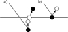 |
Fig. 1 Two model components: (a) knock-on sputtered surface atoms and (b) backscattered solar wind. The surface is indicated by the horizontal line. Solar wind particles are shown as open circles, and surface atoms as filled circles. |
2 Instrumentation
The Advanced Small Analyzer for Neutrals (ASAN) (Wieser et al. 2020) is one of the scientific instruments on the Yutu-2 rover of the Chang’E-4 mission (Jia et al. 2018) to the lunar far side. ASAN measures energetic neutral atoms emitted from the lunar surface. ASAN covers an energy range of 10 eV to 10keV with a coarse mass resolution of m/Δm ≈ 2. ASAN is a single-pixel instrument with its field of view pointing towards the lunar surface. The surface area covered is about 1 m2 in size and located between 1 m and 2 m away from the rover. Most of the time (>98%) when ASAN is operating, this area is fully illuminated by the Sun and the solar wind and not shadowed by the rover.
3 Model
The energetic neutral atoms emitted from the surface consist of reflected and neutralised solar wind and particles sputtered from the lunar regolith. The two components can be distinguished by their energy spectrum and mass composition. To constrain the physical processes involved, we constructed a semi-empirical model of the energy spectra of the energetic neutral atoms emitted from the surface.
For this model we considered only two processes generating energetic neutral atoms (Fig. 1): (a) single knock-on sputtered atoms generated by solar wind particles backscattered on a near-surface atomic layer of the regolith and (b) the backscattered solar wind protons themselves. As will be shown, these two components are sufficient to describe the observed energy spectra. The model is able to describe knock-on sputtered atoms of any species contained in the regolith, although in the present paper we focus only on hydrogen.
3.1 Knock-on sputtered atoms
The first contribution, the normalised differential flux J* in units of eV−1 of the knock-on sputtered atoms, is described using the expanded model from Kenmotsu et al. (2004); for brevity, we call this the sputtered component in the following text. For this component (Fig. 1a), a solar wind proton or alpha particle hit the surface and was first backscattered by a binary collision with an atom in a near-surface atomic layer of a regolith grain. On the way back to the surface, the backscattered particle underwent a second binary collision with a target atom located in an atomic layer closer to the surface. This target atom was then ejected from the surface (knock-on sputtered). In the following, we use index 1 for the incident projectile, index 2 for the emitted target atom, and index 3 for an atom serving as the backscattering centre located in a near-surface atomic layer of the regolith grain. The normalised differential flux J* of the emitted neutral atoms is described by
![Mathematical equation: ${J^ * }\,\left( {{E_2};{E_1},{M_1},{M_2},{M_3}} \right) = {1 \over {{k^ * }}} \cdot {{{E_2}} \over {{{\left( {{E_2} + {U_{\rm{S}}}} \right)}^{\alpha + 1}}}} \cdot \,{\left[ {\ln {{{T_{\max }}\left( {{E_1}} \right)} \over {{E_2} + {U_{\rm{s}}}}}} \right]^2},$](/articles/aa/full_html/2024/04/aa48876-23/aa48876-23-eq1.png) (1)
(1)
where E2 and M2 are the energy and mass of the ejected sputtered atom, respectively, E1 and M1 the energy and the mass of the incident particle, and M3 the mass of the near-surface atom serving as the backscattering centre. The constant, α, was taken from Lindhard’s power approximation, with α = 3/5 as in Kenmotsu et al. (2004). The normalisation constant, k*, makes the integral of J* over E2 equal to 1. Us describes the average surface binding energy, assumed to be 5 eV in our model (see for example Kudriavtsev et al. 2005). Tmax is the maximum kinetic energy of a sputtered atom and depends on the energy, E1 , of the incident particle and implicitly also on the masses, M1, M2, and M3, of the involved particles. It is modelled, as in Kenmotsu et al. (2004), as
 (2)
(2)
where γb is the energy transfer factor in the first elastic collision that backscatters the primary particle and 1 – γb is the fraction of energy that remains in the primary particle after backscat-tering near the surface on an atom with mass M3. γ is the energy transfer factor in the second elastic collision between the backscattered primary particle and the sputtered atom.
The primary particle is assumed to be backscattered towards the surface normal, with φ the angle of the incident particle to the surface normal. The two factors, 1 – γb and γ, needed to calculate the maximum kinetic energy of a sputtered particle are given by
 (3)
(3)
 (4)
(4)
The shape of the energy spectrum of the sputtered flux shown in Eq. (1) differs from the spectrum given in Sigmund (1969) by a slower than E−2 drop-off towards higher energies.
3.2 Backscattered solar wind
The second component considered consists of a solar wind proton that was directly backscattered to space by a single binary collision with a target atom in a near surface atomic layer (Fig. 1b). For brevity, we call this the scattered component in the following text.
For this component, we do not use the formalism described in Eq. (3), as the inclusion of inelastic effects is important here. The normalised differential flux, J+, in units of eV−1 of the directly backscattered hydrogen atoms is instead described empirically by an exponentially modified Gaussian, motivated by the spectrum shapes reported in Wieser et al. (2002):
 (5)
(5)
with the empirical shape parameters K = 2, a = 0.70, and b = 0.10. k+ normalises the integral of J+ over E2 to 1. The shape parameters will depend on the observation direction relative to the surface. For our model, the fit parameters were modelled for a 60° angle emission relative to the surface normal, matching the ASAN observation geometry. Other emission angles will likely result in different parameter values.
Composition model for the solar wind, SW.
3.3 The combined model
The observed energy differential neutral atom flux, J, is a weighted sum of the sputtered J* and scattered J+ flux components (Eq. (6)).
![Mathematical equation: $\matrix{ {A = \sum\limits_{{M_1}}^{SW} {\sum\limits_{{M_2}}^G {\sum\limits_{{M_3}}^R {\,s\left( {{M_1}} \right)} } } \cdot r\left( {{M_2}} \right) \cdot r\left( {{M_3}} \right) \cdot {J^ * }\left( {{E_2};{E_1},{M_1},{M_2},{M_3}} \right)} \hfill \cr {B = \left\{ {\matrix{ {{J^ + }\left( {{E_2};\,{E_1}} \right)} \hfill & {{\rm{if}}\,\,G = {\rm{H}}} \hfill \cr 0 \hfill & {{\rm{otherwise}}} \hfill \cr } } \right.} \hfill \cr {J\left( {{E_2};G,{E_1}} \right) = {J_{{\rm{sw}}}} \cdot \left[ {{k_1}\,A + {k_2}\,B} \right]} \hfill \cr } $](/articles/aa/full_html/2024/04/aa48876-23/aa48876-23-eq6.png) (6)
(6)
The sputtered component, A, is a weighted sum of fluxes originating from different combinations of primary projectiles with mass M1, sputtered atoms with mass M2, and backscattering target atoms in the regolith with mass M3. The factor, s(M1), represents the abundance of the species M1 in the solar wind, S W (Table 1). The second factor of r(M2) is the abundance of the sputtered species M2 in the regolith belonging to mass group G (from the corresponding section of Table 2). It should be noted that the sum over M2 is only over the elements in the selected mass group, G. Finally, the third factor, r(M3), is the abundance of the backscattering species M3 in the regolith, R (the whole of Table 2). As above, E1 is the energy of the solar wind ion with mass M1, and E2 the energy of the sputtered neutral atoms.
The backscattered component, B, is only relevant when the mass group, G, of interest is equal to H. For other mass groups, the J+ term vanishes, as the solar wind does not contain elements of other mass groups from Table 2 in a significant amount.
The angular constraints originating from the ASAN field of view orientation relative to the surface, the solar wind incidence angle to the surface, and the sputter yield were taken into account by the later empirically determined normalisation constants k1 = 2.5 × 10⁻⁴ sr−1 and k2 = 2.5 × 10⁻² sr−1.
The total observed energy differential flux, J, in units of cm−2 sr−1 eV−1 s−1 is proportional to the impinging solar wind number flux, JSW, in units of cm−2 s−1.
Elemental composition model for the regolith, R.
4 Data and results
The present analysis uses energetic neutral atom data obtained in the time interval from 11 January 2019 to 22 October 2020, covering a total observation time of 90 h. The data was obtained in several measurement sessions of typically 1 h in length. Due to thermal constraints on the rover, data collection was limited to two time windows around 9 h and 15 h local time on the surface. Different azimuthal scattering angles could nevertheless be investigated, as the rover’s orientation relative to the sun varied significantly (Fig. 2). ASAN never looks directly at the Sun due to its accommodation on the rover. The ASAN field-of-view boresight direction corresponds to 0° azimuth and -30° elevation in rover solar coordinates. Solar wind parameters varied quite a lot, as is shown by histograms of the most important parameters, taken from OMNI data (King & Papitashvili 2005), in Fig. 3. Despite the limited observation time of ASAN, the average distribution of solar wind parameters during the ASAN observations approximates well the average parameter distribution during the interval from 1 January 2019 to 17 March 2022.
ASAN obtains one mass spectrum for a fixed energy every 31.25 ms and then cycles through a table with 48 different energy settings. A total of 45 000 individual energy-mass spectra were used in the present analysis. In-flight performance analysis shows that the high-voltage power supply used to select the energy setting of ASAN experiences a temperature drift of on average 0.6 V K−1. This drift results in a temperature-dependent energy scale. The slow temperature changes inside of the instrument and a well-calibrated internal temperature sensor make it possible to compensate for this drift during ground data processing.
Three main signal components are present in the data: backscattered solar wind hydrogen and sputtered surface atoms as the foreground signal and a background signal attributed to gamma radiation originating from the rover’s radioisotope heater unit.
The background signal from the radioisotope heater unit on Yutu-2 partially overlaps with the energetic neutral hydrogen signal. This background signal appears as an artificial mass peak in the mass spectrum. The foreground energetic neutral atom signal was extracted by decomposing the measured mass spectrum for each energy bin into its components using a maximum likelihood fitting procedure (Kraft 1988; Le Cam 1990). Only the extracted energetic neutral hydrogen component was used in the subsequent analysis. The data also contain heavier elements but their analysis requires determination of the instrument response to Si- and Fe-group elements, which is not yet available.
The average differential energetic hydrogen number flux shown in Fig. 4a is a convolution of the actual average flux with the instrument’s energy response function. To compare the model with actual data, a model spectrum,  , was calculated, consisting of a weighted sum of the flux, J (as defined in Eq. (6)), for the different solar wind conditions present during the actual observation:
 (7)
(7)
where n is the observation number, tn the duration of the observation, and Esw,n the average solar wind proton energy during the observation number, n. After folding the model spectrum with the energy response function of ASAN, it was fitted to the measured data with the constants k1 and k2 from Eq. (6) as only free parameters. The best fit shown in Fig. 4a was obtained for k1 = 2.5 × 10⁻⁴ sr−1 and k2 = 2.5 × 10⁻² sr−1. These two values are kept fixed in the following analysis.
The contribution of each of the two components of the model prior to the convolution with the ASAN energy response function is shown in Fig. 4b, with k1 and k2 set to the same values as in Fig. 4a. The shape of the energy spectrum was found to be dependent on the solar wind speed (Fig. 5), and, to a lesser degree, on the alpha to proton number density ratio. The shape is largely independent of the local time at which the measurement was taken or of the interplanetary magnetic field conditions.
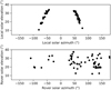 |
Fig. 2 Instrument orientation relative to the Sun. Top panel: Sun angles in a surface fixed coordinate system where 0° azimuth points towards local north and 90° azimuth to local east. The two observation windows are clearly separated, with a solar azimuth around 50° corresponding to observations during the local morning and another around −50° corresponding to observations during the local afternoon. Bottom panel: Sun position relative to a rover fixed coordinate system. |
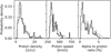 |
Fig. 3 Distribution of solar wind parameters for all the observation times used in the analysis (solid line) and for the whole time interval from 1 January 2019 to 17 March 2022 (dotted line). The data was obtained from the OMNI database. |
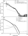 |
Fig. 4 Energy spectra of the average energetic neutral hydrogen flux. (a) Measured spectrum of the flux from the surface (black dots) compared to the instrument response to the model (grey diamonds), using data from the time interval of 11 January 2019 to 22 October 2020. Vertical error bars indicate a 90% confidence interval of the flux. Horizontal error bars represent the full width half maximum of the corresponding energy bin. The dotted line is a 90% confidence sensitivity limit (Feldman & Cousins 1998), below which the signal cannot be distinguished from zero due to the significant background that was subtracted. (b) Fitted model of energetic neutral hydrogen flux with sputtered and backscattered components separated. |
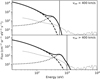 |
Fig. 5 Fitted models of energetic neutral hydrogen flux, with components separated for solar wind speeds <400 km s−1 (top) and >400 km s−1 (bottom). The solid vertical line indicates the median solar wind proton energy within the data set. The other lines have the same meaning as in Fig. 4b. |
5 Discussion
The reported high-resolution energy spectra shapes of energetic neutral hydrogen atoms emitted from the lunar surface expand the previously reported data from remote measurements. We have formulated a semi-empirical model of the shape of the energy spectrum including only two physical processes that describe the average energy spectrum of energetic neutral atoms emitted from the lunar surface. Excellent agreement between the model and the data is obtained.
Futaana et al. (2012) suggested that the low energy tail of the emitted energetic neutral hydrogen spectrum is produced by solar wind protons scattering up to 20 times in the regolith before reemission. This is in contrast to our model, where the low energy part of the distribution is predominantly generated from single collisions of backscattered solar wind protons with previously implanted hydrogen atoms, as is shown in Fig. 1a.
Despite only very sparse observations distributed over a long time interval, the statistical variations in the solar wind upstream flux and alpha to proton number density ratio were well sampled during the time interval that the data covers. Solar wind speed is the only parameter that significantly affects the spectrum shape in the available data set (Fig. 5). A higher alpha to proton number density ratio, αsw, will increase the amplitude and slightly modify the energy spectrum of the sputtered component, but due to limited sampling this effect is not visible because of the large variation in other solar wind parameters during the time the data was acquired. Heavier solar wind ions, for example multiply charged oxygen, do not notably modify the neutral hydrogen energy spectrum – their abundance is typically too low. The energy spectrum shape of the scattered component is expected to change with different incidence and emission angles, but the available data does not allow quantification of this effect due to coverage limitations.
The magnitude of both the observed sputtered and scattered flux also depends on the incidence angle of the solar wind and the emission angles of the observed particles. In the presented model, these magnitudes are described by the two constants, k1 and k2 (Eq. (6)). These constants depend on the incidence angle of the solar wind (Fig. 2, top panel) and the viewing angle to the surface (Fig. 2, bottom panel). As the angular coverage of the ASAN observations is limited, further model assumptions are needed for full angular coverage. The emission profile of the sputtered component should be reasonably well approximated by a cosine distribution, while the scattered component can be described by angular emission profiles previously reported by Vorburger et al. (2013).
Another effect modulating the observed total flux for energetic neutral hydrogen from the surface is the presence of lunar magnetic anomalies. The location of ASAN at 177.6°E and 45.4°S (Liu et al. 2019) is near the large lunar magnetic anomaly in the Aitken basin. The observed energetic neutral atom flux from the surface at the observation location is reduced by a factor of ≈2, if the magnetic anomaly is in the upstream solar wind direction (Xie et al. 2021). Due to the lack of in situ solar wind proton data at the surface, this effect was not considered for the current study. To address this, the total energetic neutral hydrogen flux from the surface could be scaled using energetic neutral atom albedo estimates, for example from Wieser et al. (2009), Vorburger et al. (2013) or Xie et al. (2021). Additionally, a correction for a possible increased surface potential that reduces the energy of the impinging solar wind (Futaana et al. 2012) could be added. Despite these limitations, the analytical formulation of the presented model allows for a straightforward implementation in lunar exosphere models (see for example Wurz et al. 2007) and an extrapolation to other solar wind parameters.
No complete elemental composition of the low-Ti regolith (Qiao et al. 2019) present at the landing site of Chang’E-4 is available as the mission was not a sample return mission. Compared to the average composition for low-Ti mare soils from Wurz et al. (2007) used as a proxy in Table 2, the soil at the landing site is depleted in Fe (Qiao et al. 2019). The effect of this on the modelled energetic neutral hydrogen spectra in Fig. 4b is negligible, however.
The model is currently only validated for emitted energetic neutral hydrogen, but future improvements in the ASAN instrument calibration for heavy energetic neutral atoms, for example in the O-, Si-, and Fe-group of elements (Table 2), will allow for verification of the generalisation of the presented model to these element groups.
Acknowledgements
The Advanced Small Analyzer for Neutrals (ASAN) instrument was developed by the Swedish Institute of Space Physics (IRF) in Kiruna, Sweden, and the National Space Science Center (NSSC) in Beijing, China, as a joint project. It is supported by the Swedish National Space Agency, SNSA, under grants 95/11 and 122/18, the National Natural Science Foundation of China (NSFC) grant 41941001, and the Beijing Municipal Science and Technology Commission under grant 181100002918003.
References
- Allegrini, F., Dayeh, M. A., Desai, M. I., et al. 2013, Planet. Space Sci., 85, 232 [NASA ADS] [CrossRef] [Google Scholar]
- Barabash, S., Bhardwaj, A., Wieser, M., et al. 2009, Curr. Sci., 96, 526 [Google Scholar]
- Berisch, R., & Wittmaack, K. 1991, in Sputtering by Particle Bombardment III, (New York: Springer-Verlag), 1 [Google Scholar]
- Crider, D. H., & Vondrak, R. R. 2002, Adv. Space Res., 30, 1869 [NASA ADS] [CrossRef] [Google Scholar]
- Feldman, G. J., & Cousins, R. D. 1998, Phys. Rev. D, 57, 3873 [NASA ADS] [CrossRef] [Google Scholar]
- Feldman, W. C., Lawrence, D. J., Elphic, R. C., et al. 2000, J. Geophys. Res., 105, 4175 [NASA ADS] [CrossRef] [Google Scholar]
- Funsten, H. O., Allegrini, F., Bochsler, P. A., et al. 2013, J. Geophys. Res. Planets, 118, 292 [NASA ADS] [CrossRef] [Google Scholar]
- Futaana, Y., Barabash, S., Wieser, M., et al. 2012, J. Geophys. Res. Planets, 117 [Google Scholar]
- Futaana, Y., Barabash, S., Wieser, M., et al., 2012, Geophys. Res. Lett., 40, 262 [Google Scholar]
- Goswami, J. N., & Annadurai, M. 2009, Curr. Sci., 96, 486 [Google Scholar]
- Jia, Y., Zou, Y., Xue, C., et al. 2018, Chinese J. Space Sci., 38, 118 [NASA ADS] [CrossRef] [Google Scholar]
- Johnson, R. E., & Baragiola, R. 1991, Geophys. Res. Lett., 18, 2169 [NASA ADS] [CrossRef] [Google Scholar]
- Kenmotsu, T., Yamamura, Y., Ono, T., & Kawamura, T. 2004, J. Plasma Fusion Res., 80, 406 [CrossRef] [Google Scholar]
- King, J. H., & Papitashvili, N. E. 2005, J. Geophys. Res., 110, A02104 [Google Scholar]
- Kudriavtsev, Y., Villegas, A., Godines, A., & Asomoza, R. 2005, Appl. Surf. Sci., 239, 273 [CrossRef] [Google Scholar]
- Kraft, D. 1988, Tech. Rep. DFVLR-FB 88-28, DLR German Aerospace Center – Institute for Flight Mechanics, Köln, Germany [Google Scholar]
- Le Cam, L. 1990, Int. Stat. Rev., 58, 153 [CrossRef] [Google Scholar]
- Liu, J., Ren, X., Yan, W. et al., 2019, Nat. Commun., 10, 1 [NASA ADS] [CrossRef] [Google Scholar]
- McComas, D., Allegrini, F., Bochsler, P., et al. 2009, Space Sci. Rev., 146, 11 [NASA ADS] [CrossRef] [Google Scholar]
- Qiao, L., Ling, Z., Fu, X., & Li, B. 2019, Icarus, 333, 37 [CrossRef] [Google Scholar]
- Rodriguez M., Saul, D. F. Wurz, L., et al. 2012, Planet. Space Sci., 60, 297 [NASA ADS] [CrossRef] [Google Scholar]
- Saul, L., Wurz, P., Vorburger, A., et al. 2013, Planet. Space Sci., 84, 1 [NASA ADS] [CrossRef] [Google Scholar]
- Schaufelberger, A., Wurz, P., Barabash, S., et al. 2011, Geophys. Res. Lett., 38 [Google Scholar]
- Sigmund, P. 1969, Phys. Rev. 184, 383 [CrossRef] [Google Scholar]
- von Steiger, R., Schwadron, N. A., Fisk, L. A., et al. 2000, J. Geophys. Res., 105 [Google Scholar]
- Vorburger, A., Wurz, P., Barabash, S., et al. 2013, J. Geophys. Res. Space Phys., 118, 3937 [NASA ADS] [CrossRef] [Google Scholar]
- Wieser, M., Wurz, P., Bruning, K., & Heiland, E. 2002, Nucl. Instrum. Meth. B, 192, 370 [Google Scholar]
- Wieser, M., Barabash, S., Futaana, Y., et al. 2009, Planet. Space Sci., 57, 2132 [NASA ADS] [CrossRef] [Google Scholar]
- Wieser, M., Barabash, S., Wang, X. D., et al. 2020, Space Sci. Rev., 216, 73 [CrossRef] [Google Scholar]
- Wurz, P., Rohner, U., Whitby, J. A., et al. 2007, Icarus, 191, 486 [NASA ADS] [CrossRef] [Google Scholar]
- Xie, L., Li, L., Zhang, A., et al. 2021, Geophys. Res. Lett., 48, e2021GL093943 [CrossRef] [Google Scholar]
- Zhou, C., Tang, H., Li, X., et al. 2022, Nat. Commun., 13, 5336 [Google Scholar]
All Tables
All Figures
|
Fig. 1 Two model components: (a) knock-on sputtered surface atoms and (b) backscattered solar wind. The surface is indicated by the horizontal line. Solar wind particles are shown as open circles, and surface atoms as filled circles. |
| In the text | |
|
Fig. 2 Instrument orientation relative to the Sun. Top panel: Sun angles in a surface fixed coordinate system where 0° azimuth points towards local north and 90° azimuth to local east. The two observation windows are clearly separated, with a solar azimuth around 50° corresponding to observations during the local morning and another around −50° corresponding to observations during the local afternoon. Bottom panel: Sun position relative to a rover fixed coordinate system. |
| In the text | |
|
Fig. 3 Distribution of solar wind parameters for all the observation times used in the analysis (solid line) and for the whole time interval from 1 January 2019 to 17 March 2022 (dotted line). The data was obtained from the OMNI database. |
| In the text | |
|
Fig. 4 Energy spectra of the average energetic neutral hydrogen flux. (a) Measured spectrum of the flux from the surface (black dots) compared to the instrument response to the model (grey diamonds), using data from the time interval of 11 January 2019 to 22 October 2020. Vertical error bars indicate a 90% confidence interval of the flux. Horizontal error bars represent the full width half maximum of the corresponding energy bin. The dotted line is a 90% confidence sensitivity limit (Feldman & Cousins 1998), below which the signal cannot be distinguished from zero due to the significant background that was subtracted. (b) Fitted model of energetic neutral hydrogen flux with sputtered and backscattered components separated. |
| In the text | |
|
Fig. 5 Fitted models of energetic neutral hydrogen flux, with components separated for solar wind speeds <400 km s−1 (top) and >400 km s−1 (bottom). The solid vertical line indicates the median solar wind proton energy within the data set. The other lines have the same meaning as in Fig. 4b. |
| In the text | |
Current usage metrics show cumulative count of Article Views (full-text article views including HTML views, PDF and ePub downloads, according to the available data) and Abstracts Views on Vision4Press platform.
Data correspond to usage on the plateform after 2015. The current usage metrics is available 48-96 hours after online publication and is updated daily on week days.
Initial download of the metrics may take a while.