


| Issue |
A&A
Volume 711, July 2026
|
|
|---|---|---|
| Article Number | A176 | |
| Number of page(s) | 8 | |
| Section | Galactic structure, stellar clusters and populations | |
| DOI | https://doi.org/10.1051/0004-6361/202660660 | |
| Published online | 14 July 2026 | |
X-shooter spectroscopy of giant stars in the nuclear star cluster★
1
INAF, Osservatorio di Astrofisica e Scienza dello Spazio di Bologna,
Via Gobetti 93/3,
40129
Bologna,
Italy
2
Dipartimento di Fisica e Astronomia “Augusto Righi”, Alma Mater Studiorum, Universitá di Bologna,
Via Gobetti 93/2,
40129
Bologna,
Italy
3
Department of Physics and Astronomy, UCLA,
430 Portola Plaza,
Box 951547,
Los Angeles,
CA
90095-1547,
USA
4
Université Côte d’Azur, Observatoire de la Côte d’Azur, CNRS, Laboratoire Lagrange,
06000
Nice,
France
5
Division of Astrophysics, Department of Physics, Lund University,
Box 118,
221 00
Lund,
Sweden
6
Fraunhofer IOSB (Institute of Optronics, System Technologies and Image Exploitation), Department Object Recognition,
Gutleuthausstr. 1,
76275
Ettlingen,
Germany
★★ Corresponding author: This email address is being protected from spambots. You need JavaScript enabled to view it.
Received:
28
April
2026
Accepted:
16
June
2026
Abstract
Near-IR spectra of a homogeneous sample of 15 red giants in the Galactic nuclear star cluster, within 1.5 pc of SgrA*, have been acquired with X-shooter at the Very Large Telescope. From these spectra, line-of-sight radial velocities and chemical abundances of iron, carbon, oxygen, and other alpha and light elements have been derived. By combining radial velocities from this study and proper motions from the literature, we computed the orbits of these stars, finding that they have been confined within 12 pc from SgrA* for their entire lifetime, thus strongly suggesting an in situ formation and evolution. Iron abundances between half and twice solar; approximately solar-scaled values within ±0.1 dex for α-elements, Ti, and V; some enhancement of [Na/Fe], [K/Fe], and [Al/Fe]; and some depletion of [C/Fe] with respect to the solar ratios have been measured. The inferred chemical abundance distributions are consistent with a formation from a gas enriched by type II and type I supernovae (SNe) over a prolonged timescale, closely matching those of the metal-rich populations of the inner bulge field and other complex stellar systems like Terzan 5 and Liller 1.
Key words: techniques: spectroscopic / stars: abundances / stars: late-type / galaxy: nucleus
Based on observations at the Very Large Telescope of the European Southern Observatory at Cerro Paranal (Chile), under programme 099.D-0258 (PI: L. Origlia).
© The Authors 2026
 Open Access article, published by EDP Sciences, under the terms of the Creative Commons Attribution License (https://creativecommons.org/licenses/by/4.0), which permits unrestricted use, distribution, and reproduction in any medium, provided the original work is properly cited.
This article is published in open access under the Subscribe to Open model. This email address is being protected from spambots. You need JavaScript enabled to view it. to support open access publication.
1 Introduction
In the era of Gaia (Gaia Collaboration 2016) and ground-based massive spectroscopic surveys of the old stellar populations in the Milky Way halo and the bulge-disc at 4–8 m class telescopes, radial velocities and chemical abundances for large samples of giant stars in the Galaxy field and star clusters are being obtained and are providing fundamental information on the formation and chemical enrichment history of the various Galactic components. A few other massive surveys are planned in the near future by using the next generation of multi-object spectrographs with unprecedented large multiplexing (Cirasuolo & MOONS Consortium 2016; de Jong et al. 2019; Jin et al. 2024) to provide a comprehensive kinematic and chemical mapping of the stellar populations of the Milky Way. Within the Galaxy, however, the innermost nuclear region towards the Galactic centre (GC) remains poorly explored despite its uniqueness and importance, for example in understanding the co-evolution and feedback of the central black hole and the surrounding host, mostly because of the extinction, which is so severe that only observations at IR and radio wavelengths are possible. APOGEE (Majewski et al. 2017) and a few other small surveys at Keck, VLT, and Gemini are making use of medium- to high-resolution red and near-IR spectroscopy to observe giant stars in the central hundreds of parsecs, in order to get chemical abundances of iron, iron-peak and neutron-capture elements, CNO, and some other alpha and light elements. In particular, measurements of cool giants in the central 500 pc from the GC (see e.g. Rich et al. 2007, 2012; Ryde et al. 2016a; Nandakumar et al. 2018; Schultheis et al. 2019, 2020; Feldmeier-Krause et al. 2020; Fritz et al. 2021; Nieuwmunster et al. 2023, and references therein) indicate iron abundances from one-third to twice solar, with a tail towards [Fe/H]<−0.5 dex and some alpha enhancement. Measurements of red supergiants and some older giants close to the GC (see e.g. Ramirez et al. 2000; Cunha et al. 2007; Davies et al. 2009; Ryde & Schultheis 2015; Nandakumar et al. 2018, and references therein) are consistent with peak metallicity around solar and a low level (if any) of alpha-element enhancement.
The Galactic nucleus discovered by Becklin & Neugebauer (1968) has since been described with greater precision by Morris & Serabyn (1996); Launhardt et al. (2002). The early star formation and chemical enrichment history of the nucleus is expected to be somewhat unique. The presence of the supermassive black hole (SMBH) should significantly affect star formation via tidal forces (see e.g. Ghez 2007; Genzel et al. 2010) and stellar orbits within its sphere of influence, while outside of it the stellar populations should be more similar to those of the inner bulge-disc. Star counts and kinematics (Schödel et al. 2014; Feldmeier et al. 2014; Fritz et al. 2016, and references therein) reveal a central compact structure, called the nuclear star cluster (NSC), with a half-light radius of 7 pc and a mass of about 2.5 × 10⁷ M⊙, that also hosts the supermassive black hole SgrA*. This NSC contains stars covering a wide range of ages and metallicities, thus suggesting a quasi-continuous star formation history. It might be the surviving core of multiple globular clusters or other stellar systems that have migrated towards the centre from outside the nuclear region (see e.g. Tremaine et al. 1975; Capuzzo-Dolcetta 1993; Antonini 2013; Gnedin et al. 2014) or it could have formed in situ (see e.g. Milosavljević 2004; Seth et al. 2008; Pflamm-Altenburg & Kroupa 2009), with the possible contribution of stars from the inner bulge and/or disc. A metallicity gradient between the NSC and the nuclear stellar disc (NSD) (see e.g. Feldmeier-Krause 2022) has also been claimed.
In order to solve the puzzle of the NSC formation and evolution, it is of fundamental importance to determine the individual abundances of iron, CNO, and other alpha, light and heavy elements of old giants, likely members of the NSC, and to compute suitable abundance ratios that are crucial in order to constrain star formation and chemical enrichment timescales. K-band spectroscopy of giant stars in the central parsec of the NSC (Do et al. 2015; Feldmeier-Krause et al. 2017) has provided overall metallicities spanning a wide range from about one-tenth to supersolar values. However, the limited spectral resolution (R~4–5000) of these observations prevented the measurement of individual chemical abundances and a proper chemical tagging of the old stellar population(s) in this environment. Ryde et al. (2016b) provide some detailed chemical abundances of iron and a few alpha elements of a metal-poor alpha-enhanced bright giant at <30 pc from SgrA*. A more comprehensive sample of giants stars in the NSC analysed by (Rich et al. 2017; Thorsbro et al. 2020) indicate iron abundances around solar with a spread of ~0.3 dex and some level of [Si/Fe] enhancement. More recently, high-resolution H- and K-band spectroscopy of a few metal-rich cool giants in the NSC (Ryde et al. 2025; Nandakumar et al. 2025) has provided chemical abundances of iron-peak and alpha elements that follow the trends of the metal-rich population in the inner bulge.
Taking advantage of the X-shooter (Vernet et al. 2011) spectrograph at the VLT with its medium-resolution and simultaneous wide spectral coverage and high throughput in the near-IR, we efficiently observed a sample of 15 stars that are likely members of the NSC and located within about 1.6 pc from the GC. The observations and data reduction are presented in Sect. 2, the spectral analysis is discussed in Sect. 3. Sections 4 and 5 present the results of our kinematic and chemical analyses, respectively, while Sect. 6 reports some final considerations and our conclusions.
Coordinates, photometry, proper motions, heliocentric radial velocities (RVs), effective temperatures, and orbital parameters for the observed NSC stars.
2 Observations and data reduction
We observed 15 giant stars, candidate members of the NSC, with X-shooter at VLT under programme 099.D-0258 (PI: L. Origlia). Because of the huge reddening towards the NSC, only the spectra acquired with the near-IR arm and the 0.6 arcsec slit (providing a resolution of R≈8000) in the 1.15–2.37 μm range were used for spectral analysis.
The targets have been extracted from the catalog of Fritz et al. (2016) by using the quoted H- and K-band photometry, right ascension (RA) and declination (Dec) coordinates and proper motions (see Table 1) and applying the following selection criteria:
- (i)
By using the observed K,H-K colour-magnitude diagram (see Fig. 1, left panel), in order to maximize the probability of selecting candidate NSC member old giants below the red giant branch (RGB) tip on the one hand, and to observe stars bright enough to get X-shooter spectra with a sufficiently high signal-to-noise ratio in a reasonable amount of integration time on the other hand, we selected stars with K in the 10–12 magnitude range and very red H-K in the 1.8–3.2 colour range to account for the huge absolute and differential reddening in that direction.
- (ii)
We selected stars located in an annular region between about 0.5 and 1.6 pc assuming a distance of 8.2 kpc (i.e. between 13 and 40 arcsec projected on sky) from the GC (see Fig. 1, middle panel) in order to sample the SMBH sphere of influence, but avoiding the innermost crowded region at r<0.5 pc, where seeing limited observations are problematic.
- (iii)
We selected stars with proper motions of |μRA| and |μDec| ≤ 5 mas/yr (see Fig. 1, right panel), thus consistent with being NSC members.
Since the selected target stars undergo an average visual extinction of about 30 mag, and are thus too faint to be detected with the X-shooter acquisition camera that works in the R band, and hence too faint to be directly centred in the slit, a blind offset from a brighter nearby reference star was used. The acquisition of X-shooter spectra was then performed by nodding on slit with a typical throw of a few arcsec, for a proper background and detector subtraction. An O-star spectrum observed during the same night was used to check and eventually remove telluric features. Typical total on-source exposure times ranged from 30 to 60 min, depending on the target brightness.
The reduction of the X-shooter near-IR spectra was performed by using the ESO X-shooter pipeline to obtain background subtracted, flatfield corrected, rectified and wavelength calibrated 2D spectra. The 1D spectrum extraction was performed manually in order to visually inspect and optimize the location and extension on the detector of the target-sky pair of spectra corresponding to the A and B positions along the slit. Due to the severe extinction towards the NSC, only the portion of the X-shooter spectra covering the H and K bands have enough signal to be effectively used for the subsequent science analysis. The signal-to-noise ratio of the final extracted spectra at λ > 1.5 μm is always >30. Figure 2 shows an example of observed spectra around some atomic and molecular lines of interest for two stars with similar stellar parameters and different metallicities.
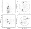 |
Fig. 1 K,H-K colour–magnitude diagram (top left), RA–Dec map (top right), heliocentric RVs as a function of the projected distance from SgrA* (bottom left) and proper motions (bottom right) for the stars towards the NSC (gray dots) measured by Fritz et al. (2016). Targets observed with X-shooter are indicated as large black dots. In the top right panel the two big circles delimit the regions at projected distances on sky of 13 and 40 arcsec, corresponding to about 0.5 and 1.6 pc, respectively, from SgrA*. In the bottom right panel, the circle has a radius of 5 mas yr−1. |
3 Spectral analysis
The R=8000 spectral resolution and the simultaneous wide near-IR spectral coverage of the calibrated X-shooter spectra, coupled with spectral synthesis and cross-correlation techniques, enabled us to estimate the stellar parameters, radial velocities, and chemical abundances of individual elements for the 15 observed stars.
The absolute and differential reddening towards the NSC is so severe, and is affected by non-negligible uncertainties, and thus prevented us from obtaining any reliable photometric estimate of the stellar temperature. Hence, as was done in previous studies of the NSC (see e.g. Rich et al. 2017; Feldmeier-Krause et al. 2017; Ryde et al. 2025; Nandakumar et al. 2025), the stellar temperatures were derived from the (2−0) and (3−1)12CO band-heads in the K band and the empirical relations of Schultheis et al. (2016), while a gravity of log g=0.5 and microturbulence of 2 km s−1, typical of luminous bulge and GC giant stars with similar low temperatures (see e.g. Rich et al. 2012, 2017), were assumed for all the observed stars. The derived temperatures in the 3200–3800 K range were also cross-checked against OH lines in order to obtain a simultaneous best fit of all the molecular CO and OH transitions.
Uncertainties in the derived stellar parameters are mostly systematic and for the observed cool giants near the RGB tip we estimated values of ±100 K in temperatures, ±0.3 dex in log(g) and ±0.2 km s−1 in microturbulence. The overall impact of these uncertainties in the derived [X/H] abundances and [X/Fe] abundance ratios is always within 0.15 dex, normally within 0.1 dex, and they have mostly the effect of rigidly shifting the chemical distributions. However, since these shifts turn out to be relatively small (if present at all), they do not significantly affect the overall appearance of the inferred distributions.
Heliocentric radial velocities (RVs) were obtained via cross-correlation of the observed spectra with suitable templates whose stellar parameters closely match those of the target stars in the 2.29–2.37 μm spectral window in the K band, which includes several CO lines and bandheads. The RV uncertainty was estimated using the full width at half maximum of the cross-correlation function combined with the signal-to-noise ratio of the observed spectra, resulting in an error of ~2 km s−1 (Tonry & Davis 1979). The derived heliocentric RVs were also crosschecked and validated with the atomic and molecular lines in the H band.
The chemical abundances were obtained via spectral synthesis techniques of suitable atomic lines and molecular features, free from significant blending with other species and/or contamination by telluric absorption and without strong wings. Although blending from other species was taken into account when using spectral synthesis, and telluric correction was applied, non-perfect modelling and/or correction may leave residuals, hence spectral regions of strong blending and/or contamination were discarded for chemical analysis. At the R=8000 resolution of X-shooter, a few reasonably clean atomic lines of NaI, MgI, AlI, SiI, KI, CaI, TiI, VI, and FeI were identified in the H and K bands and they were used to measure the corresponding element abundances. OH molecular lines and CO bandheads in the H band were used to derive O and C abundances, respectively. From 13CO bandheads in the K band (see e.g. Fanelli et al. 2021) we could also estimate the 12C/13C isotopic ratio.
Suitable grids of synthetic spectra were computed with stellar parameters similar to those of the observed stars. The metallicities ranged from [Fe/H]=−1.0 dex to [Fe/H]=+0.5 dex with a step of 0.1 dex, with some enhancement of [N/Fe] and corresponding depletion of [C/Fe] for a proper computation of the molecular equilibria, and with solar-scaled [X/Fe] values for the other elements. We used the radiative transfer code TURBOSPECTRUM (Alvarez & Plez 1998; Plez 2012), along with MARCS models atmospheres (Gustafsson et al. 2008), atomic data from the VALD3 compilation (Ryabchikova & Pakhomov 2015), and the most recent molecular data from the website of B. Plez1.
In order to match the observed line profile broadening, the synthetic spectra were convolved with a Gaussian function at the R≈8000 X-shooter resolution. This instrumental broadening dominates any other intrinsic broadening, such as macroturbulence and rotation. For an optimal pixel-to-pixel comparison between the observed and the synthetic spectra, the latter were also resampled to match the pixel size (0.6 Å) of the observed spectra. The observed spectra were normalized by using the synthetic spectra as a reference to locally (i.e. around each line of interest) place the continuum, with an overall uncertainty of ≤2%. Best-fit solutions for the chemical abundances of the various species were obtained by minimizing the scatter between the observed and synthetic spectra around each line of interest and using as a figure of merit line depth or equivalent width measurements and overall spectral synthesis. Random errors in the inferred chemical abundances are mostly due to the uncertainties in the placement of the continuum and to the photon noise. The values quoted in Table 2 were thus estimated as the dispersion around the mean abundance divided by the squared root of the number of lines used (normally a few; see Table 2) to measure each chemical element or an error of 0.1 dex is assumed if only one line is available.
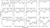 |
Fig. 2 Portions of normalized rest-frame X-shooter near-IR spectra around some atomic and molecular lines of interest for stars 5726 (solid) and 7363 (dotted) with similar stellar parameters and different metallicities. |
Chemical abundances* and corresponding errors** for the observed NSC stars.
4 Kinematics and orbits
For the observed 15 stars, we inferred the heliocentric RVs in the −124 < vhel < +127 km s−1 range, with an average value of - 4.6± 16.1 km s−1 and a dispersion of 62.5± 11.4 km s−1. Although our estimate of such a velocity dispersion is somewhat affected by low number statistics, it is fully consistent with the velocity dispersion profile obtained by Feldmeier et al. (2014), and suggests that our sample of candidate NSC stars belongs to a system that should be pressure-supported. By using these line-of-sight RVs and the corresponding tangential velocities from proper motions by Fritz et al. (2016), we also computed the orbital parameters of our stars, with the main purpose of constraining their confinement to the NSC. The orbits were computed with AGAMA (Vasiliev 2019) in the same non-axisymmetric potential adopted by Nieuwmunster et al. (2024, and references therein), which includes a triaxial bar-bulge, the NSD, and the NSC. The bar has a clockwise pattern speed Ωp = 40 km s−1 kpc−1 and an initial angle of 25° with respect to the Sun-GC line (Portail et al. 2017; Sormani et al. 2022). We fixed R0 = 8.2 kpc and performed two different integrations in the bar rotating frame: (i) an integration over 12 Gyr with a 1 Myr time step, aimed at characterizing the overall orbital confinement and long-term stability; (ii) a high-resolution integration over 500 Myr with a 4000 yr time step, to constrain the orbital morphology. Most orbits display regular, rosettelike patterns in the x–y plane, while a few show mildly boxy or elongated morphologies depending on their initial phase-space coordinates. The resulting best-fit trajectories of the two sets of simulations are confined within ≲12 pc from the GC, with rapo ≤ 11.6 pc and zmax ≤ 7.9 pc (see Table 1).
5 Chemical abundances and abundance ratios
For the observed 15 stars of the NSC, Table 2 lists the inferred chemical abundances and corresponding random errors of Fe, C, O, Na, Mg, Al, Si, K, Ca, Ti, and V and the 12C/13C isotopic ratio, by using as solar references those from Magg et al. (2022). Figure 3 shows the computed [X/H] abundances (left panels) and [X/Fe] abundance ratios (right panels) as a function of [Fe/H], with typical errors on individual element abundances of ≤0.1 dex (see Table 2). The inferred distribution of [Fe/H] values for the 15 observed stars is quite broad, spanning about 0.5 dex, from –0.15 to +0.35 dex, and with an average value of +0.12± 0.04 dex and a 1σ dispersion of 0.17±0.03 dex, significantly larger than the error of the mean and also somewhat larger than the typical <0.1 dex measurement error. Such a metallicity spread suggests that the NSC is a stellar system more complex than a genuine globular cluster. The [X/Fe] abundance ratios of O, Mg, Si, Ca, Ti, and V are about solar-scaled (within ±0.1 dex), while [Na/Fe] is enhanced with respect to the solar-scaled value. The [Al/Fe] and [K/Fe] distributions show a trend with metallicity, with more metal-poor stars being somewhat enhanced, while the more metal-rich ones being about solar-scaled. We do not find any significant dispersion of Na and/or O, and consequently no evidence of a Na–O anti-correlation, typically observed in genuine globulars (e.g. Carretta et al. 2009).
These [X/Fe] versus [Fe/H] distributions were compared to those of Liller 1, a complex stellar system of the bulge hosting multi-age and multi-metallicity stellar populations (Ferraro et al. 2021), for which a similar chemical analysis from X-shooter spectroscopy (Alvarez Garay et al. 2024; Fanelli et al. 2024) was performed. We find a nice agreement between the abundance patterns of the NSC stars and the metal-rich population of Liller 1, and more generally with the metal-rich stellar populations of the bulge and other complex stellar systems, such as Terzan 5 (see e.g. Rich et al. 2012; Origlia et al. 2011, and references therein). In particular, the [α/Fe] abundance ratios consistent with the solar-scaled values or at most with a mild enhancement, indicates that these metal-rich stars formed from a gas enriched by both type II and type I supernovae (SNe), at variance with the metal-poor components of the bulge stellar populations that show a significant [α/Fe] enhancement and likely formed more quickly from a gas mostly enriched by type II SNe. Our chemical analysis of the NSC stars is also in nice agreement with the study of Nandakumar et al. (2025) for the chemical elements in common.
Some [C/Fe] depletion (see Fig. 3) with respect to the solar-scaled value, low 12C/13C isotopic ratios between 7 and 15 (see Table 2 and Fig. 4) with a typical uncertainty of ±1, and some correlation between 12C/13C and [C/Fe] for all the observed stars have been also inferred from our study. Such a carbon depletion is typically measured in luminous giants, regardless of their metallicity, thus indicating that mixing and extra-mixing processes should be at work during the evolution along the RGB.
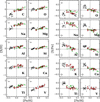 |
Fig. 3 [X/H] abundances (left panels) and [X/Fe] abundance ratios (right panels) of C, O, Na, Mg, Al, Si, K, Ca, Ti, V vs. [Fe/H] for the observed NSC stars (large red dots from this work, and green triangles from Nandakumar et al. 2025) and for Liller 1 stars (black dots) from Alvarez Garay et al. (2024), for comparison. The error bars are also marked in the left corner of each plot. |
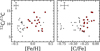 |
Fig. 4 12C/13C isotopic ratio as a function of [Fe/H] (left panel) and [C/Fe] (right panel) for the observed NSC stars (large red dots) and for Liller 1 stars (black dots) from Alvarez Garay et al. (2024), for comparison. The error bars are also marked in the top left corner ofeach plot. |
6 Discussion and conclusions
We presented our kinematic and chemical study of a homogeneous sample of 15 giant stars, all located within 0.5 and 1.6 pc from the GC, i.e. well within the half-light radius of the NSC, with line-of-sight RVs and proper motions also consistent with a NSC membership, and colour-magnitude diagrams consistent with being very reddened giants. Our study has some statistical significance to attempt a first characterization of the old stellar content of the NSC in terms of population properties.
With the purpose of evaluating whether the observed distribution of [α/Fe] (where α is the average of the O, Mg, Si, and Ca abundances) versus [Fe/H] shows some statistical evidence of multiple sub-components, we performed a Gaussian mixture model (GMM) analysis, as done by Fanelli et al. 2024 on Liller 1. Both the Bayesian and Akaike information criteria favour a single population model. We caution, however, that with only 15 stars this analysis has very limited statistical power. Hence, we also implemented a 2D ([Fe/H], [α/Fe]) hierarchical Bayesian model, using the dynesty dynamic nested sampling package and accounting for the full covariance matrix in the error budget of each star. According to this test, the single-population model is moderately favoured on the Jeffreys scale, although the existence of a more complex structuring, undetectable with the current sample size, cannot be ruled out.
The overall high metallicity slightly above solar, on average, and with significant spread, together with the rather low level (if any) of [α/Fe] enhancement (see Fig. 5) of such a population suggests that the gas from which it formed may have (self-)enriched with both type II and type I SNe ejecta on a somewhat prolonged timescale. Moreover, the kinematic confinement in the central parsecs and the striking chemical similarity with the metal-rich stellar populations of the Galactic bulge, and of other complex stellar systems located there, for example Terzan 5 and Liller 1, strongly favour an in situ formation and evolution of the NSC.
In the coming years, we have the perspective of making a true quantum step in characterizing the stellar content of the nuclear region of the Milky Way, thanks to the Galactic survey in guaranteed time with the new multi-object spectrograph MOONS (Gonzalez et al. 2020) at the VLT. More specifically, as a part of that survey, there will be an optimized sampling of the stellar populations in the central hundred parsecs, by acquiring medium- to high-resolution near-IR spectra of tens of thousands of stars distributed in the nuclear disc, bar, and bulge and of a few hundred stars in the NSC. Such a high-quality homogeneous dataset will provide the necessary statistical grounds to perform robust chemo-dynamical population studies, in order to properly identify and characterize possible sub-structures and their mutual interactions, as well as their link with the inner Galaxy.
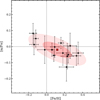 |
Fig. 5 Average [α/Fe] vs. [Fe/H] and associated error bars for the observed NSC stars (black dots), where α is the average of the O, Mg, Si, and Ca abundances. The Gaussian mixture model (GMM) best fit is superimposed; the red cross indicates the centroid (mean) of the identified component, while the concentric shaded regions are the 1σ and 2σ confidence ellipses. |
Acknowledgements
LO and CF acknowledge the financial support by INAF within the ELT-ANDES project. CF acknowledges support by the PRIN INAF 2023 grant ObFu N2RED (PI: C. Fanelli). NR acknowledges support from the Swedish Research Council (grant No. 2023-04744).
References
- Alvarez, R., & Plez, B. 1998, A&A, 330, 1109 [NASA ADS] [Google Scholar]
- Alvarez Garay, D. A., Fanelli, C., Origlia, L., et al. 2024, A&A, 686, A198 [NASA ADS] [CrossRef] [EDP Sciences] [Google Scholar]
- Antonini, F. 2013, ApJ, 763, 62 [Google Scholar]
- Becklin, E. E., & Neugebauer, G. 1968, ApJ, 151, 145 [Google Scholar]
- Capuzzo-Dolcetta, R. 1993, ApJ, 415, 616 [NASA ADS] [CrossRef] [Google Scholar]
- Carretta, E., Bragaglia, A., Gratton, R. G., et al. 2009, A&A, 505, 117 [NASA ADS] [CrossRef] [EDP Sciences] [Google Scholar]
- Cirasuolo, M., & MOONS Consortium. 2016, in Astronomical Society of the Pacific Conference Series, 507, Multi-Object Spectroscopy in the Next Decade: Big Questions, Large Surveys, and Wide Fields, eds. I. Skillen, M. Balcells, & S. Trager, 109 [Google Scholar]
- Cunha, K., Sellgren, K., Smith, V. V., et al. 2007, ApJ, 669, 1011 [NASA ADS] [CrossRef] [Google Scholar]
- Davies, B., Origlia, L., Kudritzki, R.-P., et al. 2009, ApJ, 694, 46 [NASA ADS] [CrossRef] [Google Scholar]
- de Jong, R. S., Agertz, O., Berbel, A. A., et al. 2019, The Messenger, 175, 3 [NASA ADS] [Google Scholar]
- Do, T., Kerzendorf, W., Winsor, N., et al. 2015, ApJ, 809, 143 [Google Scholar]
- Fanelli, C., Origlia, L., Oliva, E., et al. 2021, A&A, 645, A19 [NASA ADS] [CrossRef] [EDP Sciences] [Google Scholar]
- Fanelli, C., Origlia, L., Rich, R. M., et al. 2024, A&A, 690, A139 [NASA ADS] [CrossRef] [EDP Sciences] [Google Scholar]
- Feldmeier-Krause, A. 2022, MNRAS, 513, 5920 [Google Scholar]
- Feldmeier, A., Neumayer, N., Seth, A., et al. 2014, A&A, 570, A2 [NASA ADS] [CrossRef] [EDP Sciences] [Google Scholar]
- Feldmeier-Krause, A., Kerzendorf, W., Neumayer, N., et al. 2017, MNRAS, 464, 194 [Google Scholar]
- Feldmeier-Krause, A., Kerzendorf, W., Do, T., et al. 2020, MNRAS, 494, 396 [Google Scholar]
- Ferraro, F. R., Pallanca, C., Lanzoni, B., et al. 2021, Nat. Astron., 5, 311 [Google Scholar]
- Fritz, T. K., Chatzopoulos, S., Gerhard, O., et al. 2016, ApJ, 821, 44 [Google Scholar]
- Fritz, T. K., Patrick, L. R., Feldmeier-Krause, A., et al. 2021, A&A, 649, A83 [NASA ADS] [CrossRef] [EDP Sciences] [Google Scholar]
- Gaia Collaboration (Prusti, T., et al.) 2016, A&A, 595, A1 [NASA ADS] [CrossRef] [EDP Sciences] [Google Scholar]
- Genzel, R., Eisenhauer, F., & Gillessen, S. 2010, Rev. Mod. Phys., 82, 3121 [Google Scholar]
- Ghez, A. M. 2007, in Astronomical Society of the Pacific Conference Series, 367, Massive Stars in Interactive Binaries, eds. N. St.-Louis, & A. F. J. Moffat, 689 [Google Scholar]
- Gnedin, O. Y., Ostriker, J. P., & Tremaine, S. 2014, ApJ, 785, 71 [Google Scholar]
- Gonzalez, O. A., Mucciarelli, A., Origlia, L., et al. 2020, The Messenger, 180, 18 [NASA ADS] [Google Scholar]
- Gustafsson, B., Edvardsson, B., Eriksson, K., et al. 2008, A&A, 486, 951 [NASA ADS] [CrossRef] [EDP Sciences] [Google Scholar]
- Jin, S., Trager, S. C., Dalton, G. B., et al. 2024, MNRAS, 530, 2688 [NASA ADS] [CrossRef] [Google Scholar]
- Launhardt, R., Zylka, R., & Mezger, P. G. 2002, A&A, 384, 112 [NASA ADS] [CrossRef] [EDP Sciences] [Google Scholar]
- Magg, E., Bergemann, M., Serenelli, A., et al. 2022, A&A, 661, A140 [NASA ADS] [CrossRef] [EDP Sciences] [Google Scholar]
- Majewski, S. R., Schiavon, R. P., Frinchaboy, P. M., et al. 2017, AJ, 154, 94 [NASA ADS] [CrossRef] [Google Scholar]
- Milosavljević, M. 2004, ApJ, 605, L13 [Google Scholar]
- Morris, M., & Serabyn, E. 1996, ARA&A, 34, 645 [Google Scholar]
- Nandakumar, G., Ryde, N., Schultheis, M., et al. 2018, MNRAS, 478, 4374 [Google Scholar]
- Nandakumar, G., Ryde, N., Schultheis, M., et al. 2025, ApJ, 982, L14 [Google Scholar]
- Nieuwmunster, N., Nandakumar, G., Spitoni, E., et al. 2023, A&A, 671, A94 [NASA ADS] [CrossRef] [EDP Sciences] [Google Scholar]
- Nieuwmunster, N., Schultheis, M., Sormani, M., et al. 2024, A&A, 685, A93 [NASA ADS] [CrossRef] [EDP Sciences] [Google Scholar]
- Origlia, L., Rich, R. M., Ferraro, F. R., et al. 2011, ApJ, 726, L20 [CrossRef] [Google Scholar]
- Pflamm-Altenburg, J., & Kroupa, P. 2009, MNRAS, 397, 488 [CrossRef] [Google Scholar]
- Plez, B. 2012, Turbospectrum: Code for spectral synthesis, Astrophysics Source Code Library [record ascl:1205.004] [Google Scholar]
- Portail, M., Gerhard, O., Wegg, C., & Ness, M. 2017, MNRAS, 465, 1621 [NASA ADS] [CrossRef] [Google Scholar]
- Ramirez, S. V., Stephens, A. W., Frogel, J. A., & DePoy, D. L. 2000, AJ, 120, 833 [CrossRef] [Google Scholar]
- Rich, R. M., Origlia, L., & Valenti, E. 2007, ApJ, 665, L119 [NASA ADS] [CrossRef] [Google Scholar]
- Rich, R. M., Origlia, L., & Valenti, E. 2012, ApJ, 746, 59 [NASA ADS] [CrossRef] [Google Scholar]
- Rich, R. M., Ryde, N., Thorsbro, B., et al. 2017, AJ, 154, 239 [NASA ADS] [CrossRef] [Google Scholar]
- Ryabchikova, T., & Pakhomov, Y. 2015, Baltic Astron., 24, 453 [NASA ADS] [Google Scholar]
- Ryde, N., & Schultheis, M. 2015, A&A, 573, A14 [NASA ADS] [CrossRef] [EDP Sciences] [Google Scholar]
- Ryde, N., Schultheis, M., Grieco, V., et al. 2016a, AJ, 151, 1 [Google Scholar]
- Ryde, N., Fritz, T. K., Rich, R. M., et al. 2016b, ApJ, 831, 40 [Google Scholar]
- Ryde, N., Nandakumar, G., Schultheis, M., et al. 2025, ApJ, 979, 174 [Google Scholar]
- Schödel, R., Feldmeier, A., Kunneriath, D., et al. 2014, A&A, 566, A47 [Google Scholar]
- Schultheis, M., Ryde, N., & Nandakumar, G. 2016, A&A, 590, A6 [Google Scholar]
- Schultheis, M., Rich, R. M., Origlia, L., et al. 2019, A&A, 627, A152 [NASA ADS] [CrossRef] [EDP Sciences] [Google Scholar]
- Schultheis, M., Rojas-Arriagada, A., Cunha, K., et al. 2020, A&A, 642, A81 [EDP Sciences] [Google Scholar]
- Seth, A. C., Blum, R. D., Bastian, N., Caldwell, N., & Debattista, V. P. 2008, ApJ, 687, 997 [NASA ADS] [CrossRef] [Google Scholar]
- Sormani, M. C., Gerhard, O., Portail, M., Vasiliev, E., & Clarke, J. 2022, MNRAS, 514, L1 [NASA ADS] [CrossRef] [Google Scholar]
- Thorsbro, B., Ryde, N., Rich, R. M., et al. 2020, ApJ, 894, 26 [NASA ADS] [CrossRef] [Google Scholar]
- Tonry, J., & Davis, M. 1979, AJ, 84, 1511 [Google Scholar]
- Tremaine, S. D., Ostriker, J. P., & Spitzer, L., J. 1975, ApJ, 196, 407 [NASA ADS] [CrossRef] [Google Scholar]
- Vasiliev, E. 2019, MNRAS, 482, 1525 [Google Scholar]
- Vernet, J., Dekker, H., D’Odorico, S., et al. 2011, A&A, 536, A105 [NASA ADS] [CrossRef] [EDP Sciences] [Google Scholar]
All Tables
Coordinates, photometry, proper motions, heliocentric radial velocities (RVs), effective temperatures, and orbital parameters for the observed NSC stars.
All Figures
|
Fig. 1 K,H-K colour–magnitude diagram (top left), RA–Dec map (top right), heliocentric RVs as a function of the projected distance from SgrA* (bottom left) and proper motions (bottom right) for the stars towards the NSC (gray dots) measured by Fritz et al. (2016). Targets observed with X-shooter are indicated as large black dots. In the top right panel the two big circles delimit the regions at projected distances on sky of 13 and 40 arcsec, corresponding to about 0.5 and 1.6 pc, respectively, from SgrA*. In the bottom right panel, the circle has a radius of 5 mas yr−1. |
| In the text | |
|
Fig. 2 Portions of normalized rest-frame X-shooter near-IR spectra around some atomic and molecular lines of interest for stars 5726 (solid) and 7363 (dotted) with similar stellar parameters and different metallicities. |
| In the text | |
|
Fig. 3 [X/H] abundances (left panels) and [X/Fe] abundance ratios (right panels) of C, O, Na, Mg, Al, Si, K, Ca, Ti, V vs. [Fe/H] for the observed NSC stars (large red dots from this work, and green triangles from Nandakumar et al. 2025) and for Liller 1 stars (black dots) from Alvarez Garay et al. (2024), for comparison. The error bars are also marked in the left corner of each plot. |
| In the text | |
|
Fig. 4 12C/13C isotopic ratio as a function of [Fe/H] (left panel) and [C/Fe] (right panel) for the observed NSC stars (large red dots) and for Liller 1 stars (black dots) from Alvarez Garay et al. (2024), for comparison. The error bars are also marked in the top left corner ofeach plot. |
| In the text | |
|
Fig. 5 Average [α/Fe] vs. [Fe/H] and associated error bars for the observed NSC stars (black dots), where α is the average of the O, Mg, Si, and Ca abundances. The Gaussian mixture model (GMM) best fit is superimposed; the red cross indicates the centroid (mean) of the identified component, while the concentric shaded regions are the 1σ and 2σ confidence ellipses. |
| In the text | |
Current usage metrics show cumulative count of Article Views (full-text article views including HTML views, PDF and ePub downloads, according to the available data) and Abstracts Views on Vision4Press platform.
Data correspond to usage on the plateform after 2015. The current usage metrics is available 48-96 hours after online publication and is updated daily on week days.
Initial download of the metrics may take a while.