© The Authors 2026

1. Introduction

Galactic cosmic rays (CRs) are believed to be accelerated at supernova remnant (SNR) shocks (Gabici et al. 2019). However, this scenario is challenged by a number of observations. In particular, it is not clear whether SNR shocks can accelerate protons up to the PeV energy domain, as required by near-Earth observations of CRs. This is why the search for proton PeVatrons in the Galaxy is a major goal of gamma-ray astronomy (Cao et al. 2021). Despite tremendous progress, this remains an open issue.

The amplification of the magnetic field (MF) to values exceeding the interstellar one is a necessary condition for acceleration to PeV energies at SNRs (Hillas 2005). The synchrotron X-ray filaments observed at some SNR shocks demonstrate that the MF there is indeed largely amplified (Helder et al. 2012). The amplification may be due to plasma instabilities triggered by the streaming of CRs accelerated at the shock (Marcowith et al. 2021). In this scenario, the amplification takes place upstream of the shock, improves the confinement of CRs within the acceleration region, and boosts their energy to large values.

Here we show that interstellar dust grains overtaken by a shock trigger a plasma instability that may result in a large amplification of the MF. In this case, the amplification takes place downstream of the shock and therefore neither improves the confinement of CRs at SNRs nor increases their maximum energy. After comparing our predictions with observations, we conclude that this scenario may be a viable alternative to explain the large values of the MF strength observed in some SNRs.

2. Charged dust grains overtaken by shocks

Consider dust grains of mass M_g = A_gm_p and charge Q_g = Z_ge, where m_p and e are the proton mass and charge, and A_g and Z_g the grain’s analog of the atomic mass and number, respectively. For simplicity, we assume that grains are spheres of radius a.

Interstellar dust grains acquire a positive charge due to a number of processes such as the photoelectric effect, the impact of atoms, or ions on the grain’s surface (Ellison et al. 1997). As a result, grains acquire an electric potential, ϕ = Q_g/a, on the order of 10–100 V or, equivalently, a charge of

$$\begin{array}{c}\hfill Z_g=\frac{a\varphi }{e}\sim 6.9\times {10}^2\left(\frac{a}{{10}^{-5}\mathrm{cm}}\right)\left(\frac{\varphi }{10\mathrm{V}}\right).\end{array}$$(1)

The grain atomic number is

$$\begin{array}{c}\hfill A_g=\frac{4\pi }{3}{a}^3\frac{{\varrho }_g}{m_p}\sim 7.5\times {10}^9\left(\frac{{\varrho }_g}{3\mathrm{g}/{\mathrm{cm}}^3}\right){\left(\frac{a}{{10}^{-5}\mathrm{cm}}\right)}^3,\end{array}$$(2)

where 𝜚_g is the density of grain material (Cristofari et al. 2025).

Consider now grains swept up by a shock of velocity u_s. Initially, grains are not affected by the shock passage, as they are characterized by rigidities much larger than those of thermal particles. Therefore, once downstream they move with a velocity of u_g = (3/4)u_s with respect to the shocked gas. In the rest frame of the downstream fluid, the momentum of dust grains is p_g = A_gm_pu_g, corresponding to PV rigidities (R = p_gc/Z_ge) and sub-parsec scale Larmor radii (r_L = R/B₀),

$$\begin{array}{cc}\hfill \frac{R}{\mathrm{PV}}& \sim 0.13\left(\frac{u_s}{5\times {10}^8\mathrm{cm}/\mathrm{s}}\right)\left(\frac{{\varrho }_g}{3\mathrm{g}/{\mathrm{cm}}^3}\right){\left(\frac{a}{{10}^{-5}\mathrm{cm}}\right)}^2\left(\frac{10\mathrm{V}}{\varphi }\right),\hfill \\ \hfill \frac{r_L}{\mathrm{pc}}& \sim 0.05\left(\frac{u_s}{5\times {10}^8\mathrm{cm}/\mathrm{s}}\right)\left(\frac{{\varrho }_g}{3\mathrm{g}/{\mathrm{cm}}^3}\right){\left(\frac{a}{{10}^{-5}\mathrm{cm}}\right)}^2\left(\frac{10\mathrm{V}}{\varphi }\right)\left(\frac{3\mathrm{\mu }\mathrm{G}}{B_0}\right),\hfill \end{array}$$(3)

where B₀ is the MF strength downstream of the shock.

Note that, especially for young SNRs characterized by large shock speeds and small sizes, the Larmor radius of grains can be of the same order of the thickness of the SNR shell, which is a small fraction of the SNR radius. When that happens, grains are unmagnetized and cross the region suffering very little deflection. The current associated with the streaming of charged dust grains excites plasma instabilities similar to those triggered by CR streaming (Hopkins & Squire 2018). Given the similarities in the behavior of CR nuclei and charged grains, it is natural to wonder what contribution the latter makes to the amplification of MFs at shocks. Here we argue that, in some cases, dust grains might play a major role in amplifying the MF downstream of the shock, and not upstream, as CRs are believed to do.

Further downstream of the shock, grains will eventually be isotropized by the MF and, due to their large rigidities, will behave as CR nuclei. Some of them may be able to recross the shock and start to be accelerated via a first-order Fermi mechanism. This has been described in Ellison et al. (1997) and Cristofari et al. (2025), and will not be further discussed here.

3. Dust-driven streaming instability

The growth rate of the dust-driven instability was estimated here by means of an analogy with CRs. The CR streaming instability operates at shocks in two flavors: a resonant mode and a non-resonant one (Marcowith et al. 2021). For simplicity, we limited our analysis to parallel shocks, where the direction of the ordered component of the MF in the upstream plasma is parallel to the shock normal. Both streaming instabilities are driven by a k × B force, where j is a current resulting from the streaming of charged particles, and B is the ambient MF. When a small perturbation, B₁, is added perpendicular to the ordered background field, B₀, the current will be also perturbed as j = j₀ + j₁, where j₁ ≪ j₀ and j₀ ∥ B₀. The resonant instability is driven by the j₁ × B₀ force (Kulsrud & Pearce 1969), and the non-resonant one by the j₀ × B₁ force (Bell et al. 2013). The non-resonant instability grows faster, and therefore we discuss it further.

Assume that all dust grains are identical and characterized by the same size, mass, and charge, and that their density in the interstellar medium is n_g. A generalization to the case of a broad distribution of sizes (and therefore masses and charges) is provided in Appendix A. We anticipate that larger grains are more effective in triggering the instability. As the size distribution of grains roughly scales as n_g(a)∝a^−3.5 (Mathis et al. 1977), their integral mass distribution is proportional to a × n_g(a)×A_g ∝ a^0.5 and is dominated by the largest grains. Therefore, the grain mass density in the ambient medium, 𝜚_dust = n_gA_gm_p, is the parameter determining the effectiveness of the instability.

Dust grains crossing the shock surface from upstream generate a current in the downstream frame equal to

$$\begin{array}{c}\hfill j_0=n_g{Q}_g{u}_g=\left(\frac{3e}{4}\right)Z_g{n}_g{u}_s.\end{array}$$(4)

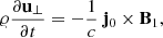
The current is parallel to the shock normal and directed downstream. As dust grains are characterized by very large rigidities, their Larmor radius can be safely assumed to be much larger than the wavelength of perturbations of the MF. Under these circumstances, j₁ = 0, and the equation of motion for the background thermal gas reads

$$\begin{array}{c}\hfill \varrho \frac{\partial {\mathbf{u}}_{\perp }}{\partial t}=-\frac{1}{c}{\mathbf{j}}_0\times {\mathbf{B}}_1,\end{array}$$(5)

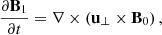
where u_⊥ is the velocity of the plasma orthogonal to B₀, 𝜚 its (constant) density, and the minus sign on the right-hand side indicates that the force is induced by a return current carried by the background plasma to balance j₀. When combined with the ideal MHD equation for the evolution of the MF,

$$\begin{array}{c}\hfill \frac{\partial {\mathbf{B}}_1}{\partial t}=\mathrm{\nabla }\times ({\mathbf{u}}_{\perp }\times {\mathbf{B}}_0),\end{array}$$(6)

it gives the two equations

$$\begin{array}{c}\hfill \frac{{\partial }^2{B}_x}{\partial t^2}=\frac{B_0{j}_0}{\varrho c}\frac{\partial B_y}{\partial z},\frac{{\partial }^2{B}_y}{\partial t^2}=-\frac{B_0{j}_0}{\varrho c}\frac{\partial B_x}{\partial z},\end{array}$$(7)

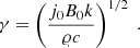
where z (x, y) indicate the directions parallel (perpendicular) to B₀. These equations show that harmonic (∝e^ikz) and right-hand circularly polarized modes are unstable and grow at the rate of

$$\begin{array}{c}\hfill \gamma ={\left(\frac{j_0{B}_{0}k}{\varrho c}\right)}^{1/2}.\end{array}$$(8)

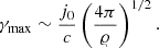
A distinct signature of the instability is that small-scale (large k) perturbations grow faster. The smallest possible scale at which the instability operates is determined by the equilibrium between the Lorentz force (j₀ × B₁/c) that drives the instability, and the magnetic tension of field lines ((B₀ ⋅ ∇)B₁/4π) that opposes that. This condition is satisfied for k_max ∼ (4π/c)j₀/B₀, which can be substituted in Eq. (8) to give the fastest growth rate:

$$\begin{array}{c}\hfill {\gamma }_{\max }\sim \frac{j_0}{c}{\left(\frac{4\pi }{\varrho }\right)}^{1/2}.\end{array}$$(9)

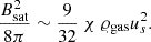
If we now impose that the scale of the perturbation should be smaller than the grain Larmor radius (otherwise grains would gyrate around the perturbed field and the Lorentz force would average to zero) we obtain a condition on the current, j₀ > B₀²c/4πR, which can be inverted to obtain the maximum possible value of the MF, B_sat, at which the instability saturates. This can be written in a convenient form introducing the ambient (interstellar) dust-to-gas ratio, χ = 𝜚_dust/𝜚_gas, giving

$$\begin{array}{c}\hfill \frac{B_{\mathrm{sat}}^2}{8\pi }\sim \frac{9}{32}\chi {\varrho }_{\mathrm{gas}}{u}_s^2.\end{array}$$(10)

The equation shows that the magnetic pressure downstream is a small fraction of the shock ram pressure, and that the proportionality constant is on the order of the dust-to-gas mass ratio. Type Ia supernovae (SNe) explode at random places in the interstellar medium, so they would encounter gas with a typical dust-to-gas ratio of χ ≲ 0.01 (Jenkins 2009). The value of χ is more uncertain for core collapse SNe. Supernovae with red supergiant progenitors would encounter a dusty circumstellar medium until they were to grow beyond the size of the progenitor star wind, which could be on the order of ≈1 pc (Van Dyk 2025). The SNe from stripped progenitors, Type Ib/c, might or might not encounter dusty circumstellar material. Normalizing χ to the typical interstellar value, we get

$$\begin{array}{c}\hfill B_{\mathrm{sat}}\sim 2\times {10}^2{\left(\frac{\chi }{0.01}\right)}^{1/2}{\left(\frac{n_H}{{\mathrm{cm}}^{-3}}\right)}^{1/2}\left(\frac{u_s}{5\times {10}^3\mathrm{km}/\mathrm{s}}\right)\mathrm{\mu }\mathrm{G},\end{array}$$(11)

where n_H is the hydrogen density in the interstellar medium (of mean atomic weight μ ∼ 1.4). Remarkably, this is quite close to the MF strengths inferred from the observations of X-ray filaments at SNR shocks (Helder et al. 2012).

So far, we have implicitly assumed that the background plasma is cold, which means that the Larmor radius of thermal particles, r_L, i (i = p or e for protons and electrons, respectively), is much smaller than 1/k_max, or r_L, ik_max → 0. However, the plasma downstream of a SNR shock is heated to a large temperature, k_BT = (3/16)m_pu_s², where k_B is the Boltzmann constant, resulting in a large thermal velocity of protons, $v_{T,p}=\sqrt{2k_{B}T/m_p}=\sqrt{3/8}{u}_s$, and a correspondingly large Larmor radius. One should consider instead, then, a situation in which r_L, pk_max is small but not vanishing. The Larmor radius of thermal electrons can still be set equal to zero as r_L, e ≪ r_L, p. A finite Larmor radius means that protons in the plasma are less magnetized, and this results in a reduction of both the instability growth rate, γ_max, and the wavenumber, k_max (Reville et al. 2008; Marret et al. 2021).

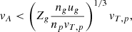
It can be shown that thermal effects are important if the plasma Alfvèn speed is (Zweibel & Everett 2010)

$$\begin{array}{c}\hfill v_A<{\left(Z_g\frac{n_g{u}_g}{n_p{v}_{T,p}}\right)}^{1/3}{v}_{T,p},\end{array}$$(12)

where n_p is the downstream ambient proton density. After some manipulations, and making use of Eq. (10), this can be rewritten as a condition on the MF immediately downstream of the shock (i.e., before the dust-driven field amplification):

$$\begin{array}{c}\hfill B_d<{\left(\frac{4}{3}\frac{Z_g}{A_g}\right)}^{1/3}\frac{B_{\mathrm{sat}}}{{\chi }^{1/6}}\sim 1{\left(\frac{A_g/Z_g}{{10}^7}\right)}^{-1/3}{\left(\frac{\chi }{0.01}\right)}^{-1/6}\left(\frac{B_{\mathrm{sat}}}{100\mathrm{\mu }\mathrm{G}}\right)\mathrm{\mu }G,\end{array}$$

which shows that thermal effect are probably quite small. This is because the minimum possible value of B_d can be estimated by assuming that no field amplification operates upstream. In that case B_d will be equal to the upstream MF for a parallel shock and four times that for a perpendicular strong shock. In both cases one expects values exceeding the microgauss level. For this reason, in the following we neglect thermal effects.

Finally, the instability operates provided that dust grains are not decelerated due to friction with the background plasma (Draine & Salpeter 1979). Ellison et al. (1997) showed that direct collisions between grains and plasma ions dominate the friction and that the corresponding momentum-loss time is τ_loss ≈ A_g/μa²n_pu_g. For typical parameters, this corresponds to stopping length τ_lossu_g on the order of a few parsecs, which is orders of magnitude larger than the width of X-ray filaments (≈10¹⁷ cm; Helder et al. 2012). This shows that friction can be neglected and that the instability will lead to an amplification of the MF.

As the amplification mechanism operates downstream, a shift will exist between the position of the shock and the peak of the MF strength, and as a consequence also a shift between the shock position and the X-ray filament, or a broadening of X-ray filaments (depending on the exact profile of the MF downstream). When the dust-driven instability is responsible for the amplification, the strength of the MF perturbation grows by a factor of e in a time of ${\gamma }_{\max }^{-1}$. The time needed to reach saturation is then τ_B = N_e/γ_max, where N_e represents the number of e-foldings of the MF. Heuristic arguments suggest that N_e ≈ 5 (Schure & Bell 2013). In a time, τ_B, the downstream fluid will move away from the shock at a speed of u_s/4, and therefore the shift will be Δl_B ≈ τ_Bu_s/4, or

$$\begin{array}{c}\hfill \mathrm{\Delta }{l}_B\approx {10}^{17}\left(\frac{N_e}{5}\right)\left(\frac{{10}^{-12}{\mathrm{cm}}^{-3}}{n_g}\right){\left(\frac{n_H}{{\mathrm{cm}}^{-3}}\right)}^{1/2}\left(\frac{{10}^{-5}\mathrm{cm}}{a}\right)\left(\frac{10\mathrm{V}}{\varphi }\right)\mathrm{cm}.\end{array}$$

The presence of a small (arcseconds) shift between the SNR shock and the X-ray emission might be detected by means of the observation of Hα filaments that do trace the position of the shock (Heng 2010). Unfortunately, cospatial Hα and X-ray filaments are rare (Heng 2010; Knežević et al. 2017; Sankrit et al. 2008; Sapienza et al. 2024), and to our knowledge no combined analysis of their spatial profiles has been performed.

4. Comparison with observations

In comparing our predictions with data we noticed that, with the exception of χ, all quantities appearing in Eq. (10) are measurable. Therefore, we made use of the compilation of data for eight young Galactic SNRs from Helder et al. (2012), and derived the value of the dust-to-gas mass ratio that one would need to explain the observed MFs in terms of the dust-driven instability discussed here. The values of χ obtained in this way are plotted in Fig. 1, where the shaded region indicates the range of typical interstellar values (Jenkins 2009), which are appropriate at least for SNRs with a type Ia progenitor.

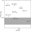Fig. 1. Dust-to-gas mass ratio (χ) needed to explain the observed values of the MF strength downstream of some SNRs. The shaded region indicates typical interstellar values for χ.

Figure 1 shows that, in order to explain the observed MF strengths, χ should be in the range of ≈0.5 − 6%. Cas A is the only object for which χ is smaller than 1%, for G1.9+0.3 χ ∼ 0.01, and for all the other objects larger values are required. G1.9+0.3 and Cas A are the two youngest SNRs in our sample. The former is most likely the result of a type Ia SN (Chakraborti et al. 2016), and the latter a type IIb (Krause et al. 2008). As Cas A is the SNR characterized by the largest value of the MF and also by the smallest (and very plausible) required value of the dust-to-gas ratio, we discuss it in more detail.

Cas A exploded about 350 years ago and its forward shock is sweeping up dusty gas over a substantial part of its area (De Looze et al. 2024). However, not all of the circumstellar gas is dusty. Koo et al. (2020) studied at a high spectral resolution a circumstellar clump that has not yet been processed by the SNR shock and found that iron was undepleted in the photoionization precursor, suggesting an absence of dust. Therefore, even though further studies are needed to determine the circumstellar value of the dust-to-gas mass ratio, a large value of χ is not implausible, at least in a sizeable fraction of the upstream material.

Competing mechanisms for MF amplification must be discussed. In particular, CRs escaping from Cas A can amplify the MF upstream of the shock (Bell et al. 2013). In assessing the importance of such a mechanism, we noticed that the gamma-ray emission observed from Cas A is strongly suppressed above a photon energy of $E_{\gamma }^{\max }\approx 1$ TeV (Cao et al. 2025). If the emission is the result of the decay of neutral pions produced in inelastic interactions of CR protons with ambient matter, then the spectrum of accelerated protons cuts off at E_max ≈ 10 TeV. This very fact implies that dust grains of larger (sub-PV, see Eq. (3)) rigidities will not be scattered effectively by MF turbulence.

The maximum energy of protons accelerated via diffusive shock acceleration at a SNR can be estimated by equating their diffusion length upstream of the shock, D(E)/u_s, to a small fraction of the shock radius, ηR_s. Here, D(E) = (1/3)r_Lc is the Bohm CR spatial diffusion coefficient and the geometric factor, η, is small and often assumed to be ≈0.05 (Ptuskin & Zirakashvili 2005). This gives a value for the upstream MF equal to

$$\begin{array}{c}\hfill \frac{B_{\mathrm{up}}}{\mathrm{\mu }\mathrm{G}}\approx 1.4{\left(\frac{\eta }{0.05}\right)}^{-1}{\left(\frac{R_s}{3\mathrm{pc}}\right)}^{-1}{\left(\frac{u_s}{5000\mathrm{km}/\mathrm{s}}\right)}^{-1}\left(\frac{E_{\max }}{10\mathrm{TeV}}\right),\end{array}$$(13)

where we normalized physical quantities to values appropriate for Cas A (Helder et al. 2012). This value is quite small and indicates that mechanisms of MF amplification operating upstream of the shock (not necessarily CR-driven, see e.g., Beresnyak et al. 2009) are not very effective. Compression at the shock may enhance the downstream MF above the value indicated in Eq. (13). However, the large scale MF in Cas A is predominantly radial (Mercuri et al. 2025), thereby limiting the impact of shock compression. This suggests that the MF amplification may well operate downstream of the shock.

Several MF amplification mechanisms may operate downstream of shocks. Vorticity is produced downstream of a warped shock interacting with a medium characterized by large-scale density fluctuations. Such vorticity can in turn distort, stretch, and eventually amplify the MF (Giacalone & Jokipii 2007). Amplification could also result from the advection of magnetic turbulence through the shock (Zank et al. 2021). Note that these mechanisms do not require the presence of CRs, but may still compete with the dust-driven mechanism proposed in this paper.

We conclude by discussing another interesting object: the type IIb SN 1993J, for which estimates of the MF have been obtained based on radio observations (Fransson & Björnsson 1998), implying a scaling in time of the downstream MF of the form B_d = B_*(t/days)⁻¹, with B_* ≈ 180 G (Tatischeff 2009). Note that this would be the same scaling predicted by Eq. (10) for a shock moving at a speed of u_s ∝ R_s/t across the progenitor stellar wind of density profile 𝜚_gas ∝ R⁻², provided that the dust-to-gas ratio χ is uniform in space. An order-of-magnitude estimate of χ can be obtained by assuming that the progenitor stellar wind is characterized by a mass loss rate of Ṁ ≈ 5 × 10⁻⁵ M_⊙/yr and a speed of u_w ≈ 10 km/s. Recalling that ϱ_gas = Ṁ/4πu_wR² and making use of Eq. (10), we get χ ≈ 0.1, which is quite large. Therefore, unless the progenitor wind is very dusty, other amplification mechanisms have to be invoked in this case.

5. Discussion and conclusion

We have shown that a dust-driven streaming instability can operate downstream of SNR shocks. In some cases the resulting MF amplification might explain the presence of the narrow X-ray filaments observed at SNR shocks. In this scenario, the MF upstream of the shock is not amplified and CRs are confined less effectively, which prevents their acceleration to PeV energies. Cas A fits particularly well within this framework, being characterized by a strong MF downstream of the shock (∼250 μG) and a low value for the maximum energy of accelerated CRs (∼10 TeV). The instability might also explain the large values of the MF observed in other SNRs, most notably G1.9+0.3.

The main point raised in this paper is the fact that, under some circumstances, the observation of strong MFs at SNR shocks does not necessarily imply that favorable conditions for the acceleration of CRs to ultrahigh energies are present. However, for systems different than SNRs, such as stellar wind termination shocks, the situation can be different. In this case, the wind blown by a star is decelerated at a slowly expanding termination shock (Morlino et al. 2021; Gabici 2024). Therefore, the downstream region is outside of the spherical shock (and not inside, as in SNRs). For dusty stellar winds, the instability discussed in this paper might indeed improve the confinement within the acceleration region (i.e., the wind termination shock), and possibly boost acceleration of particles to larger energies. It would be interesting to extend the present study to these systems.

Finally, as the MF amplification takes place downstream, it might facilitate the reflection of particles back towards the shock upstream and play a role in the complex process of injection into the acceleration mechanism (Caprioli & Spitkovsky 2014). We plan to go beyond the analytic approach presented here and to perform numerical simulations (hybrid particle-in-cell codes, Aunai et al. 2024) to better characterize the instability and its effects on SNR shock environments.

Acknowledgments

We thank F. Calura, J. Duprat, M. Lemoine, M. Miceli, G. Morlino, and B. Schroer for useful discussions.

References

Appendix A: Size distribution of dust grains

Here we generalize Eq. 10 to the case of non identical grains. Two parameterizations are widely used in the literature to describe the size distribution of grains: a scale free power-law distribution (Mathis et al. 1977), and a flatter, non-scale-free, parameterization (Weingartner & Draine 2001). The latter requires to specify more free parameters but is more accurate as it reproduces the extinction of stellar light in the Milky Way. The former is most likely oversimplified but still useful to perform order of magnitude estimates.

Mathis et al. (1977) assumed that the size distribution of grains is n(a)∝a^−3.5 in the range a_min ≡ 5 × 10⁻⁷ cm < a < 2.5 × 10⁻⁵cm ≡ a_max. One can see from Eq. 3 that the smallest grains are characterized by small Larmor radii, and therefore do not contribute to the current as they are easily isotropized. However, such small grains carry a little fraction of the total mass of interstellar dust. We therefore introduce a minimum size a_j of grains which are substantially contributing to the current. When this is done the mass density of interstellar mas dust-to-gas ratio can be written as

$$\begin{array}{c}\hfill \chi \equiv \frac{{\varrho }_{\mathit{dust}}}{{\varrho }_{\mathit{gas}}}=\frac{1}{{\varrho }_{\mathit{gas}}}{\displaystyle {\int }_{a_{\mathit{min}}}^{a_{\mathit{max}}}}\mathrm{d}an(a)\frac{4\pi }{3}{a}^3{\varrho }_g\propto a_{\mathit{max}}^{0.5},\end{array}$$(A.1)

while the current carried by grains reads (Eq. 4)

$$\begin{array}{c}\hfill j_0=\left(\frac{3e}{4}\right)u_s{\displaystyle {\int }_{a_j}^{a_{\mathit{max}}}}\mathrm{d}a{Z}_g(a)n(a)\propto a_j^{-1.5},\end{array}$$(A.2)

where the proportionalities are to be considered as approximate and are reported only to illustrate that the largest grains carry most of the mass while the smallest ones (among those which are not isotropized) carry most of the current (exact expressions will be used below). This statement holds even more strongly if one adopts the grain size distribution by Weingartner & Draine (2001), which is flatter.

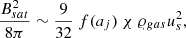
At this point, we can follow the same rationale as in Sec. 3 and assume that the instability is quenched when the Larmor radius of dust grains in the amplified MF becomes of the same size of the perturbation, and therefore grains are isotropized. A difference with respect to the case of identical grains is that when this condition is satisfied for grains of size a_j, larger grains will still contribute to the current. We therefore assume that the instability stops when the current drops by a factor of e. Under these assumptions Eq. 10 can be rewritten as

$$\begin{array}{c}\hfill \frac{B_{\mathit{sat}}^2}{8\pi }\sim \frac{9}{32}f(a_j)\chi {\varrho }_{\mathit{gas}}{u}_s^2,\end{array}$$(A.3)

where f(a_j) is a correction factor that accounts for the broad distribution of dust grain sizes and reads

$$\begin{array}{c}\hfill f(a_j)=\frac{1}{3}{a}_j^2\frac{a_j^{-3/2}-a_{\mathit{max}}^{-3/2}}{a_{\mathit{max}}^{1/2}-a_{\mathit{min}}^{1/2}}{[(1-\frac{1}{e}){\left(\frac{a_j}{a_{\mathit{max}}}\right)}^{3/2}+\frac{1}{e}]}^{-4/3},\end{array}$$(A.4)

which reaches a maximum value f ∼ 0.50 at a_j, max ∼ 0.57 × 10⁻⁵ cm. The maximum of the function is broad, and for a_j, ref = 10⁻⁵ cm (the reference grain size adopted in the paper) one gets f ∼ 0.43. If we use Eq. A.3 instead of Eq. 10 to derive the value of χ needed to explain the MF strength measured in Cas A, we get χ ∼ 1.1 − 1.2% for a_j, max < a < a_j, ref.

Smaller values of χ are expected if the flatter and more accurate grain size distribution from Weingartner & Draine (2001) is adopted. This is because the resulting mass distribution is even more peaked towards large grains. Even though this distribution depends on several free parameters, for large values of the grain size it roughly behaves as a power-law plus an exponential cutoff, with an index of the power law which is in general smaller than 3.5, and with a maximum (cutoff) size that might even be larger than the a_max fixed by Mathis et al. (1977). Both this things would reduce the value of χ required to explain the large MF observed in Cas A.

As we are interested in large grains only (small grains carry a small fraction of the mass and most likely do not contribute to the current as they are easily isotropized), to mimic the effects of a more realistic size distribution of grains we repeat the calculation above for a flatter size distribution n(a)∝a⁻³, keeping the value of a_max unchanged (assuming a larger value would lower even more the value of χ). When this assumption is done, one gets χ ∝ a_max and $j_0\propto a_j^{-1}$. Repeating the procedure above for Cas A one gets a_j, max = 0.67 × 10⁻⁵ cm and values of the dust-to-gas mass ratio χ = 0.77 − 0.84% for a_j, max < a < a_j, ref.

All the values of χ obtained above are plausible, and within less than a factor of ∼2 from what obtained by using Eq. 10, which is therefore quite accurate.

All Figures

	Fig. 1. Dust-to-gas mass ratio (χ) needed to explain the observed values of the MF strength downstream of some SNRs. The shaded region indicates typical interstellar values for χ.
In the text

References

- Aunai, N., Smets, R., Ciardi, A., et al. 2024, Comp. Phys. Commun., 295, 108966 [Google Scholar]
- Bell, A. R., Schure, K. M., Reville, B., & Giacinti, G. 2013, MNRAS, 431, 415 [Google Scholar]
- Beresnyak, A., Jones, T. W., & Lazarian, A. 2009, ApJ, 707, 1541 [NASA ADS] [CrossRef] [Google Scholar]
- Cao, Z., Aharonian, F. A., An, Q., et al. 2021, Nature, 594, 33 [NASA ADS] [CrossRef] [Google Scholar]
- Cao, Z., Aharonian, F., Bai, Y. X., et al. 2025, ApJ, 982, L33 [Google Scholar]
- Caprioli, D., & Spitkovsky, A. 2014, ApJ, 783, 91 [CrossRef] [Google Scholar]
- Chakraborti, S., Childs, F., & Soderberg, A. 2016, ApJ, 819, 37 [Google Scholar]
- Cristofari, P., Tatischeff, V., & Chabot, M. 2025, A&A, 693, A145 [NASA ADS] [CrossRef] [EDP Sciences] [Google Scholar]
- De Looze, I., Milisavljevic, D., Temim, T., et al. 2024, ApJ, 976, L4 [NASA ADS] [CrossRef] [Google Scholar]
- Draine, B. T., & Salpeter, E. E. 1979, ApJ, 231, 77 [NASA ADS] [CrossRef] [Google Scholar]
- Ellison, D. C., Drury, L. O., & Meyer, J.-P. 1997, ApJ, 487, 197 [NASA ADS] [CrossRef] [Google Scholar]
- Fransson, C., & Björnsson, C.-I. 1998, ApJ, 509, 861 [NASA ADS] [CrossRef] [Google Scholar]
- Gabici, S. 2024, in Foundations of Cosmic Ray Astrophysics, eds. F. A. Aharonian, E. Amato, P. Blasi, & C. Evoli (Amsterdam: IOS Press), 223 [Google Scholar]
- Gabici, S., Evoli, C., Gaggero, D., et al. 2019, Int. J. Mod. Phys. D, 28, 1930022 [CrossRef] [Google Scholar]
- Giacalone, J., & Jokipii, J. R. 2007, ApJ, 663, L41 [Google Scholar]
- Helder, E. A., Vink, J., Bykov, A. M., et al. 2012, Space Sci. Rev., 173, 369 [NASA ADS] [CrossRef] [Google Scholar]
- Heng, K. 2010, PASA, 27, 23 [Google Scholar]
- Hillas, A. M. 2005, J. Phys. G Nucl. Phys., 31, R95 [NASA ADS] [CrossRef] [Google Scholar]
- Hopkins, P. F., & Squire, J. 2018, MNRAS, 479, 4681 [CrossRef] [Google Scholar]
- Jenkins, E. B. 2009, ApJ, 700, 1299 [Google Scholar]
- Knežević, S., Läsker, R., van de Ven, G., et al. 2017, ApJ, 846, 167 [Google Scholar]
- Koo, B.-C., Kim, H.-J., Oh, H., et al. 2020, Nat. Astron., 4, 584 [NASA ADS] [CrossRef] [Google Scholar]
- Krause, O., Birkmann, S. M., Usuda, T., et al. 2008, Science, 320, 1195 [NASA ADS] [CrossRef] [Google Scholar]
- Kulsrud, R., & Pearce, W. P. 1969, ApJ, 156, 445 [NASA ADS] [CrossRef] [Google Scholar]
- Marcowith, A., van Marle, A. J., & Plotnikov, I. 2021, Phys. Plasmas, 28, 080601 [Google Scholar]
- Marret, A., Ciardi, A., Smets, R., & Fuchs, J. 2021, MNRAS, 500, 2302 [Google Scholar]
- Mathis, J. S., Rumpl, W., & Nordsieck, K. H. 1977, ApJ, 217, 425 [Google Scholar]
- Mercuri, A., Greco, E., Vink, J., Ferrazzoli, R., & Perri, S. 2025, ApJ, 986, 6 [Google Scholar]
- Morlino, G., Blasi, P., Peretti, E., & Cristofari, P. 2021, MNRAS, 504, 6096 [NASA ADS] [CrossRef] [Google Scholar]
- Ptuskin, V. S., & Zirakashvili, V. N. 2005, A&A, 429, 755 [NASA ADS] [CrossRef] [EDP Sciences] [Google Scholar]
- Reville, B., Kirk, J. G., Duffy, P., & O’Sullivan, S. 2008, Int. J. Mod. Phys. D, 17, 1795 [Google Scholar]
- Sankrit, R., Blair, W. P., Frattare, L. M., et al. 2008, AJ, 135, 538 [Google Scholar]
- Sapienza, V., Miceli, M., Petruk, O., et al. 2024, ApJ, 973, 105 [Google Scholar]
- Schure, K. M., & Bell, A. R. 2013, MNRAS, 435, 1174 [NASA ADS] [CrossRef] [Google Scholar]
- Tatischeff, V. 2009, A&A, 499, 191 [NASA ADS] [CrossRef] [EDP Sciences] [Google Scholar]
- Van Dyk, S. D. 2025, Galaxies, 13, 33 [Google Scholar]
- Weingartner, J. C., & Draine, B. T. 2001, ApJ, 548, 296 [Google Scholar]
- Zank, G. P., Nakanotani, M., Zhao, L. L., et al. 2021, ApJ, 913, 127 [NASA ADS] [CrossRef] [Google Scholar]
- Zweibel, E. G., & Everett, J. E. 2010, ApJ, 709, 1412 [NASA ADS] [CrossRef] [Google Scholar]