


| Issue |
A&A
Volume 711, July 2026
|
|
|---|---|---|
| Article Number | A260 | |
| Number of page(s) | 12 | |
| Section | Galactic structure, stellar clusters and populations | |
| DOI | https://doi.org/10.1051/0004-6361/202660236 | |
| Published online | 21 July 2026 | |
TOPoS
VII. Age−metallicity relation in the Galactic halo and assembly of the Milky Way
1
LIRA, Observatoire de Paris, Université PSL, Sorbonne Université, Université Paris Cité, CY Cergy Paris Université, CNRS,
92190
Meudon,
France
2
Univ Rennes, CNRS, IPR (Institut de Physique de Rennes) – UMR 6251,
35000
Rennes,
France
3
Dipartimento di Fisica e Astronomia, Università degli Studi di Firenze,
Via G. Sansone 1,
50019,
Sesto Fiorentino,
Italy
4
Department of Physics and Astronomy, University of Bologna,
Via Gobetti 93/2,
40129
Bologna,
Italy
5
INAF, Astrophysics and Space Science Observatory,
Via Gobetti 93/3,
40129
Bologna,
Italy
6
European Southern Observatory,
Casilla
19001,
Santiago,
Chile
7
Universidad Andres Bello, Facultad de Ciencias Exactas, Departamento de Física y Astronomía – Instituto de Astrofísica, Autopista Concepción-Talcahuano
7100,
Talcahuano,
Chile
8
LIRA, Observatoire de Paris, Université PSL, Sorbonne Université, Université Paris Cité, CY Cergy Paris Université, CNRS,
75014
Paris,
France
9
UPJV, Université de Picardie Jules Verne,
33 rue St Leu,
80080
Amiens,
France
10
INAF/Osservatorio Astrofisico di Arcetri,
Largo E. Fermi 5,
50125
Firenze,
Italy
★ Corresponding author.
Received:
3
April
2026
Accepted:
8
June
2026
Abstract
Context. One technique for determining stellar ages is to compare the position of a star in the Hertzsprung-Russell diagram to theoretical stellar evolutionary tracks. The sub-giant evolutionary stage is the one that is most sensitive to age and allows the most precise evolutionary age estimates.
Aims. The TOPoS sample of stars with metallicities derived from low-resolution Sloan Digital Sky Survey spectra contains a large subset of sub-giant stars with precise parallaxes from the Gaia mission, for which evolutionary ages can be determined. Our aim is to use this stellar sample to investigate the age-metallicity relation in the Galactic halo.
Methods. We use the Bayesian inference code SPInS and theoretical BaSTI stellar evolutionary tracks to determine the ages for TOPoS stars.
Results. There is a clear increase in metallicity with decreasing age, albeit with a considerable scatter at any given age. At ages larger than 8 Ga, the scatter is so large that in fact, over this range, age and metallicity appear to be uncorrelated. At any given age, the metallicity distribution is multi-modal, with up to three distinct peaks. These peaks trace three age-metallicity relations that we tentatively identify with the halo, thick-disc, and thin-disc.
Conclusions. Our data demonstrate the important role of mergers in the evolution of the Galaxy, up to 8 Ga ago. In more recent times, the spread in metallicity drops. One possibility is that the major merger Gaia-Sausage-Enceladus may have perturbed the galaxies in the Milky Way vicinity in such a way as to decrease the merger rate. Chemical evolution models and cosmological models of the Local Group both support the importance of mergers in the early evolution of the Milky Way. Larger, unbiased samples, or at least with well-understood biases, of stars with accurate ages are required for a quantitative comparison between models and data.
Key words: stars: abundances / stars: evolution / Galaxy: evolution / Galaxy: formation / Galaxy: halo / Galaxy: kinematics and dynamics
© The Authors 2026
 Open Access article, published by EDP Sciences, under the terms of the Creative Commons Attribution License (https://creativecommons.org/licenses/by/4.0), which permits unrestricted use, distribution, and reproduction in any medium, provided the original work is properly cited.
This article is published in open access under the Subscribe to Open model. This email address is being protected from spambots. You need JavaScript enabled to view it. to support open access publication.
1 Introduction
In a previous paper of the series (Bonifacio et al. 2021), we exploited the stars that were used to select candidate extremely metal-poor stars for high resolution spectroscopic observations of the TOPoS project (Caffau et al. 2013) in order to derive the metallicity distribution function of the Galactic halo. In this paper, we want to exploit a subset of that sample in order to investigate the age-metallicity relation (AMR) in the Galactic halo.
The metallicity of the gas in galaxies is related to the stellar mass and star formation rate (SFR) of the galaxy. This relation is smooth and can be modelled by a second degree polynomial (Equation (2) of Mannucci et al. 2010). For galaxies with high stellar masses (above about 1010 M⊙) the gas metallicity is essentially independent of the SFR, but for lower masses the metallicity decreases with increasing SFR (Ellison et al. 2008; Mannucci et al. 2010). This is because a high SFR is generally driven by infalling gas, but this gas also dilutes the metals in the galaxy gas phase, thus leading to a lower gas phase metallicity. Lilly et al. (2013) developed a model of galaxy evolution that naturally implies that gas metallicity is a function of stellar mass and SFR. This function is capable of fitting the data of Mannucci et al. (2010), thus providing some theoretical support to the empirical relation. Their model also considers the effects of outflows that are proportional to the SFR; however, they conclude that the fraction of mass in gas to the mass in stars does not depend on the outflows but only on the efficiency of star formation and on the SFR per unit stellar mass.
There is an exception to this general rule and that is the case for the smaller galaxy in a minor merger (Michel-Dansac et al. 2008). In this case the gas raising the SFR comes from the larger galaxy that, before the merger starts, has higher metallicity. Thus, the infalling gas is pre-enriched and the smaller galaxies show, on average, a metallicity that is about 0.2 dex higher than an isolated galaxy of the same stellar mass.
The age-metallicity relation is a property of a galaxy that depends on its SFR and on the evolution of its mass, and therefore its merger history. The models discussed above do not consider explicitly merging and assume that the mass increase of a galaxy is only due to the inflow of gas and dark matter from the environment of the galaxy. The age-metallicity relation is an output of models of galactic evolution and comparison of models to observations provides insight into the galactic history. Our aim is to provide a set of stars against which various models can be tested.
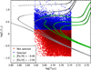 |
Fig. 1 Colour magnitude diagram of the TOPoS stars with those we analyse as SGs in blue, the others in red. To guide the eye we superimpose three BaSTI (Pietrinferni et al. 2021) isochrones with ages 4, 8, and 12 Ga and [Fe/H]=−0.4 (green) and −2.5 (grey). |
2 Target selection
We decided to focus on the sub-giant (SG) stars in the 'good parallax' sample of Bonifacio et al. (2021), because this is the evolutionary stage that is most sensitive to age. The selection of potential SG stars was done on the absolute magnitude, as G0,abs < 4.2. The selection results in a sample of 14 682 unique stars, where abundances from multiple observations of the same star have been averaged as described in Bonifacio et al. (2021); the selection is displayed in Fig. 1. It is clear that for the more metal-rich stars in our selection we also include turn-off and main sequence stars; as we go to more metal-poor stars the selection is increasingly dominated by turn-off and SG stars. The temperature cut is such that we do not include young metal-poor turn-off stars if they exist. However, we would capture young metal-poor SGs. As discussed in (Bonifacio et al. 2012) and (Caffau et al. 2013), the blue colour cut (g – z)0 ≥ 0.18, which appears in Fig. 1 as a temperature cut, was made to exclude most of the white dwarfs. One should also keep in mind that the analysis of Sloan Digital Sky Survey (SDSS) spectra for stars of low metallicity warmer than 6500 K is extremely challenging due to the weakness of the lines. With this selection, the majority of the stars are SGs, regardless of their age or metallicity. When we discuss the AMR, we return to the question of whether this selection may introduce any bias.
In Appendix A we detail how we estimate luminosities and associated errors from the data in the catalogue of Bonifacio et al. (2021). In order to limit our sample to stars of good enough quality, we only select stars with an error in the logarithmic luminosity less than 0.1. This results in a sample of 8737 stars. One could suspect that the cut in luminosity error would greatly favour nearby stars, thus leaving the more distant stars under-sampled. If we focus on the halo stars, which are typically more distant, we note that in the sample of 14 682 stars, 29% are halo stars; however, in the sample of 8737 stars, 22% are halo. Therefore, the halo is indeed slightly under-represented in our smaller sample.
3 Determining ages using SPInS
We used the logarithm base 10 of effective temperatures and luminosities, as well as metallicities, from Bonifacio et al. (2021) as input to SPInS (Lebreton & Reese 2020; Reese & Lebreton 2020; Casamiquela et al. 2024) to derive ages for our sample of stars. The choice of different projection planes does not substantially change the results, as shown, for example, by Bonifacio et al. (2024, Figure 5) and by the generally good agreement with the results of Casamiquela et al. (2024, see Sect. 3.1 and Sect. 3.2), who used absolute magnitudes, colours, and metallicities. We assumed an error of 0.018 in the logarithm of effective temperature that corresponds to about 250 K for Teff = 5900 K. The uncertainties in the correspondence between colours and effective temperatures are those implied in the determination of effective temperatures by Bonifacio et al. (2021, see there for details). For our sample, the age error does not correlate with errors in the effective temperature, luminosity, or [Fe/H]. Instead, it strongly correlates with the luminosity: the higher the luminosity, the smaller the error.
As set of stellar evolutionary tracks we chose the α-element enriched ([α/Fe] = +0.4) BaSTI ones (Pietrinferni et al. 2021), which take into account atomic diffusion, and we imposed a flat prior on ages between 0 and 13.8 Ga, which prevents finding ages older than the age of the Universe (Planck Collaboration VI 2020). To check the impact of these assumptions, we also determined ages with no priors, both with BaSTI stellar models based on a solar-scaled mixture (Hidalgo et al. 2018) and with α-enhanced models. This test showed that the general picture and the conclusions do not depend on either hypothesis. Without prior on ages, the usable sample is reduced by about 40% since one has to remove all non-physical ages, but the age-metallicity relation remains, by and large, the same. To illustrate this in Appendix B, we compare the age-metallicity relation using the ages derived with and without prior. When ages are determined without any prior, the subset of stars with ages larger than the age of the Universe, the non-physical subset, have a fainter lower magnitude than the complementary subset: brightest stars G = 13.8 while they are G = 12.8 for the complementary subset. The non-physical subset also has larger absolute magnitudes, 2.6 for the brightest stars compared to 1.3 for the physical set. For a given colour and metallicity, the older the age, the larger (i.e. fainter) the absolute magnitudes of the stars in the SG branch stage. Therefore, this behaviour of SPInS with and without prior on age is understandable.
To be more quantitative in the impact of the choice of α-enhanced evolutionary tracks, we compared the derived ages with those obtained using solar-scaled evolutionary tracks. The two correlate extremely well: a linear fit provides a correlation coefficient of 0.997, a slope very close to one (0.983) and an offset of −0.02 Ga, in the sense that ages derived from solar-scaled tracks are 0.02 Ga younger than those derived from α-enhanced tracks. The RMS around this linear fit is 0.24 Ga. The fact that both the offset and the RMS are much smaller than the median error in ages (2.35 Ga) convinced us that the choice of the α-enhanced tracks does not introduce any bias.
We must bear in mind that the ages derived from the theoretical tracks depend on the physics underlying the computations (see e.g. Lebreton et al. 2014). By imposing a prior, we force the derived ages to span the cosmological range of ages.
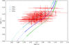 |
Fig. 2 Hertzsprung-Russell diagram for the SG stars of NGC6397 that we used to estimate its age. Three BASTI isochrones of 12, 13, and 14 Ga and metallicity −2.0 are shown for reference. |
3.1 Test with NGC 6397
To test SPInS in this configuration, we determined the age of the globular cluster NGC6397 from SGs in the sample of González Hernández et al. (2009). We cross-matched these stars with Gaia, assuming a reddening of E(B – V) = 0.186 (Gratton et al. 2003), an extinction in the G magnitude of 0.79705, derived from the KOALA grid of ATLAS 9 models (Mucciarelli et al. 2026), and 1.289445 in the GBP – GRP colour as used by Bonifacio et al. (2021). Next we used the sub-sample of stars from Bonifacio et al. (2021) to derive an empirical calibration between (GBP – GRP)0 and (g – z)0. The best fit provides (g – z)0 = −0.6193062 + 1.4829282(GBP – GRP)0. We then used the same calibration as in Bonifacio et al. (2021) to estimate the effective temperatures. We used Equation (A.7) to estimate the luminosity of the star, assuming a bolometric correction for the G magnitude of −0.02352, estimated from the synthetic colours of the KOALA grid at metallicity −2.0, and a parallax of 0.415 ± 0.01 mas (Vasiliev & Baumgardt 2021). The luminosity error was estimated from Equation (A.8). For the error on log(Teff) we assumed an error of 250 K on Teff. The resulting Hertzsprung-Russell (HR) diagram is shown in Fig. 2. We ran SPInS on these 81 stars with the same configuration as for our sample of field stars and obtained a mean age of 12.3 Ga with a standard deviation of 0.2 Ga over the 81 stars. Since SPInS relies on a Markov chain Monte Carlo (MCMC), its output consists of a distribution of possible ages, which implies that for each age determination there is an associated error. The mean error for our 81 stars is 0.9 Ga. This can be compared with the result of Casamiquela et al. (2024), who using SPInS found a mean age of 13.292 Ga from 83 stars in this cluster. As discussed in section 3.2, there are several differences between our setup of SPInS and that used by Casamiquela et al. (2024); however, the most relevant is the prior on age. To check this, we ran SPInS a second time without any prior on age for our sample. In this case, the mean age was 13.9 Ga with a dispersion of 0.5 Ga; the mean error was 2 Ga, confirming that without the age prior the errors are inflated. Moreover, this result is closer to that of Casamiquela et al. (2024), confirming that the most relevant difference in our SPInS setup lies in the prior on age.
It should be noted that all of these age estimates are compatible with each other within their errors. They are also compatible, within errors, with the ages found in the literature for NGC6397 that are assembled in Table 1.
Age estimates for NGC6397.
3.2 Comparison with Casamiquela et al
Casamiquela et al. (2024) derived ages using SPInS for a large sample of stars with metallicities from LAMOST (Cui et al. 2012). Since the LAMOST low-resolution data is similar to the SDSS (York et al. 2000) spectra we used, it is reasonable to compare our results. For this reason, we only compare this with the Low-Resolution Spectroscopic Survey (LRS) sample of Casamiquela et al. (2024). The main differences between our setup for SPInS and that of Casamiquela et al. (2024) are: (i) we use α-enhanced stellar models with a constant [α/Fe] = +0.4, while Casamiquela et al. (2024) use solar-scaled stellar models and scale the metallicity using the relation of Salaris et al. (1993); (ii) we use a prior on ages, while they use no prior; (iii) we use log(Teff), log(L), and metallicity as input to SPInS, while Casamiquela et al. (2024) use Gabs, GBP – GRP, and metallicity.
In Fig. 3, we show the comparison of the AMR of our sample, with and without prior on age, and that of Casamiquela et al. (2024). The effect of the prior on the ages is very obvious; however, note that for ages smaller than the age of the Universe the morphology of the AMR with or without prior is very similar. It is clear that our ages without prior are, by and large, consistent with those of Casamiquela et al. (2024). The two samples differ in their metallicity distributions.
This is illustrated in Fig. 4. As discussed in Bonifacio et al. (2021), while the SDSS sample is highly biased towards metal-poor stars, here it appears that the LRS sample of Casamiquela et al. (2024) is heavily biased towards solar metallicity stars. Since Casamiquela et al. (2024) did not introduce any metallicity cut in their sample, this bias must arise from the LAMOST selection function. Although we do not have kinematical data for the Casamiquela et al. (2024) sample that allows us to classify the stars of Casamiquela et al. (2024) in a way similar to what we did for our sample, we believe that it is very likely that the sample of Casamiquela et al. (2024) is dominated by disc stars, hence their metallicity distribution.
 |
Fig. 3 AMR from our sample assuming a prior on age (green dots), our sample without any prior (red dots), and the sample of Casamiquela et al. (2024) (blue dots). Note that there are red dots and blue dots below the green dots. |
 |
Fig. 4 Metallicity histogram of our sample (blue), compared with the LRS sample of Casamiquela et al. (2024) (green). The two histograms have been normalised by the number of stars in each sample. |
4 The age-metallicity relation and the assembly of the halo
We first classified the stars dynamically. The selections are the same as discussed in Bonifacio et al. (2021). Following Bensby et al. (2014) we define the stars that belong to the thin and thick disc as well as the stars that are intermediate between the thin and thick disc. The Toomre diagram is shown in Fig. 5. As a sanity check we show in Fig. 6 the Toomre diagram for the whole sample of SGs, without any cut in luminosity. It can be appreciated that, although slightly under-represented in our selection, the halo is well present. Therefore, we believe our selection does not miss any of the prominent components of the halo. We define the Gaia-Sausage-Enceladus (GSE) (Belokurov et al. 2018; Haywood et al. 2018; Helmi et al. 2018) and Sequoia accreted components (Barbá et al. 2019; Koppelman et al. 2019; Myeong et al. 2019; Villanova et al. 2019) as in Feuillet et al. (2021). The result of the selections is shown in Fig. 7.
 |
Fig. 5 Toomre diagram that we used to select thin disc and thick disc stars. |
 |
Fig. 7 Dynamically selected populations in the angular momentum-energy plane. The grey points are all the stars that cannot be classified as disc (thick or thin), GSE, or Sequoia. The grey points plus Sequoia, plus GSE, is what can generically be called halo. The units for energy are 103 × km2 s2 (actually it is a specific energy, or energy per unit mass) and 103 × kpc km s−1 for the angular momentum. |
 |
Fig. 8 AMR as defined from our dataset. The data are divided into six age bins, and for each bin we show the points corresponding to the centre of the bin and to the metallicity of the peaks. The vertical bars correspond to the FWHM of a Gaussian to each peak. The blue dots correspond to the low-AMR, the red dots to the mid-AMR, and the purple points to the high-AMR. |
 |
Fig. 9 Histogram of the metallicities in the age bin 10–12 Ga. The fitted Gaussians are shown both individually (blue, red, magenta lines) and summed (black line). |
4.1 Different age–metallicity relations
We can now look at the AMR shown in Fig. 8. At this stage, we may wonder if our selection has in some way biased our diagram. At any given metallicity, the younger populations are found among turn-off and SG stars. Since our selection favours these evolutionary stages for metal-poor stars bias would manifest as an excess of young stars at low metallicity. Since this is not the case, we conclude that our selection does not introduce any significant bias in this diagram. The probable reason is that the stars in our selection that are not SGs are a minority. To help the interpretation of the diagram we divided the sample into six age bins, and for each bin we noted the metallicity of obvious peaks in the metallicity histogram and their FWHM, both estimated by a Gaussian fit. The histograms show three, partially overlapping, peaks in the three lowest metallicity bins and only two peaks for the remaining metallicity bins. As an example, in Fig. 9 we show the histogram of the metallicities in the age bin 10 Ga to 12 Ga. We are well aware that these multiple peaks appear only due to the bias of the SDSS spectra boosting the number of stars of low metallicity (see Figure 10 of Bonifacio et al. 2021). However, here we are not trying to derive a metallicity distribution function, and we do not make any inference from the relative number of stars in any peak. We are trying to infer the AMR, and it is fairly obvious that our sample suggests at least three AMRs. For ease of discussion, in the following we refer to the three as low-AMR, mid-AMR, and high-AMR, respectively.
To gain further insight let us look at the same plot, but this time including only the stars classified as GSE (Fig. 10) and thick disc (Fig. 11). In the first case, it is obvious that the GSE stars follow the low-AMR. The thick disc instead comprises both stars that follow the low-AMR and stars that follow the mid-AMR. The thin disc stars follow in part the high-AMR and in part the mid-AMR (see Fig. 12). If we look at the age-metallicity plot with stars classified as Sequoia, they also follow by and large the low-AMR, and perhaps are defining an AMR at even lower metallicity (Fig. 13). The stars classified as halo, which also include all the GSE and Sequoia stars, follow the low-AMR, with a minority of stars that remain in the mid-AMR (Fig. 14).
We assigned to each star the probability of belonging to each of the three AMRs, using the Gaussian fits in each age bin, and then assigned it to the AMR to which it had the highest probability of belonging. In Table 2 we provide the percentages of the components in each AMR. It is clear that the high-AMR is dominated by the thin disc and the low-AMR is dominated by the halo. The mid-AMR is also dominated by the halo, but slightly less than the low-AMR and with a slightly larger fraction of disc stars, mainly thick but also a few thin. The thick disc stars are distributed almost equally among the three AMRs, for each of which they constitute in the order of one-quarter of the stars.
Belokurov et al. (2018) estimate that the GSE accretion event occurred between 8 and 11 Ga ago, while our GSE stars span a larger range extending to more than 13 Ga. These two facts are not contradictory: in fact, it is expected that the GSE progenitor was forming stars well before the accretion event. On the other hand, the fact that we do not find stars younger than 8 Ga is consistent with the accretion time estimated by Belokurov et al. (2018), since after the accretion GSE must have lost its gas and stopped forming stars.
Our AMR is morphologically similar to that provided by Gallart et al. (2019, see their Figure 3, left panel), although there is a clear shift in age and metallicity between the two. For metallicities the shift can be easily ascribed to the different techniques used: in our case the analysis of spectra, in the case of Gallart et al. (2019) the analysis of the colour magnitude diagram (CMD) and the different samples used. In the sample of Gallart et al. (2019) the most metal-poor stars are at metallicity around −1.50, whereas in our sample we go down to metallicity −3.0. This is due to the increase of the number of metal-poor stars in the SDSS spectroscopic sample, already discussed by Bonifacio et al. (2021). The shift in ages can be ascribed to two different factors. The first is methodological, as in Gallart et al. (2019) their CMD fitting procedure provides as output the age-metallicity distribution and the SFR as a function of time. This procedure suffers from age-metallicity degeneracy, as old metal-poor stars can have the same position in the CMD as younger stars of higher metallicity. However, fitting the whole CMD, from below the TO to the tip of Red Giant Branch (RGB) minimises this degeneracy. In our case, we do not have a degeneracy because of the spectroscopic determination of metallicities. The other difference is the selection process: while the sample of Gallart et al. (2019) is limited to a sphere of about 2kpc, centred on the Sun, our sample covers a larger volume and is not symmetric, having more stars towards the Galactic anticentre than towards the Galactic centre. Both of these facts could contribute to the fact that our sample has a larger number of stars younger than 6 Ga, which are very rare in the sample of Gallart et al. (2019). Nevertheless, when we look at Figure 3 of Gallart et al. (2019) it is fairly obvious that with increasing age the spread of metallicity increases, which is what we mean by saying that the two age-metalllicity relations are morphologically similar.
Another striking thing in Fig. 8 is that if we look at the data for individual stars with ages older than about 8 Ga there does not appear to be a clear correlation between age and metallicity, while at younger ages there appears to be a clear correlation. It is due to the analysis of the histograms and their peaks that we were able to define the three AMRs described above.
To assess the robustness of the multi-modality of the metallicity distributions in each age bin we analysed the three oldest age bins, where multiple peaks are visible in the metallicity histogram: 8-10 Ga, 10-12 Ga, and 12-14 Ga using routines from the scikit-learn library (Pedregosa et al. 2011). Each bin was subject to a bootstrapping analysis. In each bin the original data was used to generate a new dataset of the same size, obtained by random selection in the original set, with replacement. This means that in each bootstrap sample there are some duplicated points and some points are missing. We computed 100 bootstrap samples for each age bin. In each of the bootstrap samples three peaks were present, although in the 12–14 Ga age bin the three peaks are less distinct. We then proceeded to an error-aware bootstrap analysis; in this case, each point was not simply picked up from the original dataset but was modified by adding to it a Gaussian error that was randomly picked among the available errors. Although the histogram results are smoothed by this exercise, the three-peak structure persists. As a further test we used a Gaussian mixture model (GMM). For each age bin we used both the Akaike information criterion (Akaike 1974, AIC) and the Bayesian information criterion (Schwarz 1978, BIC) to decide whether the two- or three-component model was to be preferred. In each case, the AIC and BIC values were very close to each other, giving little discriminating power. Furthermore, the results were mixed: for the age bin 8–10 Ga three components were preferred by both criteria; for the 10-12 Ga age bin AIC favours three components and BIC prefers two components; finally for the bin with ages > 12 Ga both criteria prefer the two-component model. What is of essence here is that in any case the GMM analysis supports the existence of multi-modality in the data. Since the GMM is of little help in deciding whether two or three components are preferred, we assume that the third peak is also a distinct component, as indicated by both bootstrapping analyses.
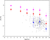 |
Fig. 10 As Fig. 8, but now only the stars classified as GSE are shown. The meaning of the colours of the dots is the same as in Fig. 8. |
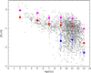 |
Fig. 11 As Fig. 8, but now only the stars classified as thick disc are shown. The meaning of the colours of the dots is the same as in Fig. 8. |
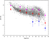 |
Fig. 12 As Fig. 8, but now only the stars classified as thin disc are shown. The meaning of the colours of the dots is the same as in Fig. 8. |
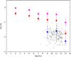 |
Fig. 13 As Fig. 8, but now only the stars classified as Sequoia are shown. The meaning of the colours of the dots is the same as in Fig. 8. |
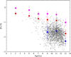 |
Fig. 14 As Fig. 8, but now only the stars classified as halo are shown. The meaning of the colours of the dots is the same as in Fig. 8. |
Percentage of stars classified as thin disc, thick disc, and halo along with each of the three AMRs.
4.2 A plausible scenario
We want to present a scenario that may explain the current observations. In the first 4 Ga the evolution of the Milky Way saw the formation of a disc, but also a large number of minor mergers, like Sequoia. Each of these dwarf galaxies had its own star formation history and metallicity distribution (see e.g. Salvadori et al. 2015). This explains the large dispersion of the metallicities observed in this age range. Each of the merging galaxies had its AMR and the low-AMR is the average of all these relations. To complicate the picture, we must also consider that the merging galaxies were gas-rich. Starbursts were likely triggered in the merging process (see e.g. Yang et al. 2024), further increasing the spread of metallicity, extending it to higher metallicities than those found in the merging galaxy prior to the beginning of the merging process.
The fact that the mid-AMR and high-AMR seem to be associated with the discs suggests that they trace the growth of metallicity in these two major structures of the Milky Way. This also suggests that the disc was not homogeneous but that there were regions of the disc that were increasing their metallicity at higher rates than others. The mid-AMR and high-AMR are an average of the lower and higher rates of growth in metallicity.
The collision between the Milky Way and the GSE progenitor, a major merger, occurred about 8 Ga to 10 Ga ago. This event likely triggered a starburst both in the incoming progenitor (see e.g. Wang et al. 2024), and in the Milky Way, whose disc was heated and formed what is now the thick disc. Mergers always trigger a starburst, although the associated star formation may be a small fraction of the total SFR of the galaxy (Wang et al. 2019). It is possible that the arrival of the GSE progenitor also had an effect on the population of dwarf galaxies and star clusters that were powering the minor merger episodes, either by accelerating their merger with the Milky Way or ejecting them so that they became unbound.
Although the present data do not directly support a causal connection between the decrease in metallicity dispersion and the GSE merging, the temporal coincidence of the two facts is intriguing and suggests speculation that they are indeed connected.
Merger simulations with sufficient spatial resolution are needed to assess the viability of this scenario. For younger ages our sample seems to be entirely constituted by disc stars.
The fact that a few of the stars of the thick disc, at low metallicities, follow the low-AMR suggests that some of the stars accreted in the merger process ended up in disc orbits as also suggested by Mori et al. (2025). In the same way, the fact that some of the halo stars follow the high-AMR suggests that in the collision processes some of the stars originally in the disc ended up in halo orbits. This is consistent with the finding of Belokurov et al. (2020) of the so-called Splash population, which is made up of metal-rich stars (metallicity larger than −0.7) in halo orbits. Although for Belokurov et al. (2020) it was possible to isolate the metal-rich component of this population, because they used APOGEE as a source of metallicities, there is no physical reason why more metal-poor stars, if present in the disc at the time of the perturbing merger, should not also be sent into halo orbits. In our sample we highlight the presence of such stars at any metallicity. It is important to remember that our dynamical groups are defined independently of the chemical composition. This scenario also explains why purely kinematical, purely chemical, or mixed selections of Galactic components define different sets of stars as shown by Franchini et al. (2020). Last but not least, it is worth noting that part of the scatter in the AMR for ages older than 8 Ga and metallicities lower than [Fe/H]= −1 may be driven by inhomogeneous enrichment during the earliest stages of galaxy formation (e.g., Vanni et al. 2023; Rossi et al. 2024).
In Fig. 15, we show for the two extreme age bins (youngest, blue, and oldest, red) the contour plots in the plane of the Galactocentric cylindrical radius and the absolute value of z. This shows clearly that the younger stars in our sample tend to concentrate at lower |z| and preferentially at Galactocentric radii larger than the Sun, consistent with an inside-out formation scenario for Galactic discs (e.g. Larson 1976; Baker et al. 2025).
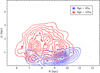 |
Fig. 15 Contour plot of the two extreme age bins (youngest and oldest) in the R, |z| plane. |
4.3 Blue metal-poor stars
For a long time, astronomers have been intrigued by the population of 'blue metal-poor' (BMP, hereafter) stars, which should contain a mixture of blue straggler stars (BSS hereafter) and intermediate age metal-poor populations. Preston et al. (1994) wanted to select metal-poor field stars with main sequence gravities, thus excluding horizontal branch stars, and to do so they introduced a photometric selection criterion based on Johnson UBV bands. In our case, we transformed the SDSS photometry to Johnson photometry1 and corrected for reddening using the extinction in the SDSS catalogue. The selection of BMP stars is shown in Fig. 16 and it consists of 3583 stars, which is 41% of the sample. The first consideration is that the majority of BMP stars are metal-poor (MP;1, 52% have −1.5 ≤ [Fe/H] ≤ −0.5). In the second place young metal-poor stars, or BSS, defined as BMP stars with age ≤10 Ga and MP, are only 46% of the BMP stars. This fraction rises to 57% if we also add the VMP and EMP stars to the sample. These stars have masses between 0.78 M⊙ and 1.4 M⊙, and 10% of these have masses larger than 1.0 M⊙. These characteristics are compatible with the BSS nature of these stars. In the sample of Preston & Sneden (2000) the BSS were estimated to be 50% of the sample, which matches very well the 46% or 57% found in our sample. The BMP stars are not necessarily young or BSS. In fact, 29% of our BMP sample have ages older than 10 Ga. Finally, in our sample, there is a total lack of young metal-poor stars, with masses above 1.6 M⊙ that can hardly be interpreted as BSS without invoking fusions of triple systems (Bonifacio et al. 2024). Several such stars have been found in the high speed sample of Bonifacio et al. (2024) and in the high radial velocity samples of Caffau et al. (2024, 2025), and Katz et al. (2025). We interpret this fact as due to the rarity of this population, that we selected a rapid evolutionary phase (SGs), and because our sample is small.
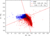 |
Fig. 16 Stars in our sample that classify as blue metal-poor according to the criteria of Preston et al. (1994). |
5 Comparison with chemical evolution models of the Milky Way and dwarf galaxies
In Fig. 17, we present the AMRs for the solar neighbourhood (SN), the Sagittarius (Sgr) dwarf spheroidal galaxy, the Sculptor (Scl) dwarf spheroidal galaxy, and the Boötes I (Boo I) ultra-faint dwarf predicted by pure galactic chemical evolution models that have been presented and extensively discussed elsewhere (Romano & Starkenburg 2013; Romano et al. 2015; Mucciarelli et al. 2017; Spitoni et al. 2019, 2021). The model predictions are compared with the relations defined from our dataset (see previous sections). The star symbols on the Sgr, Scl, and Boo I tracks indicate the points at which star formation is truncated in the models.
The divergence in the theoretical tracks reflects the fundamental differences in star formation efficiency, gas accretion history, and the impact of galactic winds across varying mass scales. The Boo I model (model Boo 7 of Romano et al. 2015) represents an ultra-faint dwarf galaxy with a stellar mass of 5.5 × 10⁴ M⊙ and a stellar metallicity distribution peaking at [Fe/H] ≃ −2.6 dex. The Scl model (model Scl T of Romano & Starkenburg 2013) represents a dwarf galaxy with a stellar mass more than two orders of magnitude larger than that of the ultra-faint, and a stellar metallicity distribution peaking at [Fe/H] ≃ −1.6 dex. The Sgr model aims at reproducing the main properties of the Sgr dwarf spheroidal galaxy at infall, namely, a rather massive object with a stellar mass of 7 × 10⁸ M⊙ and a stellar metallicity distribution peak at around [Fe/H] ≃ −0.6 dex.
The SN model (magenta line) exhibits the most rapid chemical enrichment, reaching solar metallicity within the first few billion years, when the in situ inner halo and thick-disc components form. A distinct feature of the model is the discontinuity at approximately 10.5 Ga ago. This 'kink' is consistent with a dual-infall scenario, where a second episode of pristine gas accretion dilutes the interstellar medium before the onset of the thin-disc formation phase. The fact that the data are underpopulated in the region of the kink does not necessarily signal a discrepancy between the data and the model, as we know that our observational sample is biased against solar-metallicity stars (see Bonifacio et al. 2021). The Sgr model (light blue line) shows a protracted enrichment history. Although it eventually reaches near-solar metallicities around 5 Ga ago, its track remains systematically below the SN model for the majority of cosmic time. This is indicative of an SFR that is lower than the SN and, at the same time, a potential well that is deeper than that of the smaller dwarfs, allowing for continued enrichment despite periodic gas loss, mainly due to the interaction with the Milky
Way in our model (see Mucciarelli et al. 2017). In fact the model assumes a very massive dark matter halo for the Sgr progenitor (6 × 10¹⁰ M⊙). In the model the mass loss is tuned to reproduce the observed abundances and it must be understood as the sum of the mass loss driven by supernova events in the galaxy and tidal stripping from the interaction with the Milky Way. In the low-mass regime, the Scl (medium blue) and Boo I (dark blue) models demonstrate the effects of galactic strangulation on chemical evolution. The Boo I track reaches a metallicity plateau at [Fe/H] ≈ −1.8 after star formation halts, due to delayed Fe production from SNeIa. This behaviour is typical of ultra-faint dwarfs, where early feedback from the first supernovae and the effects of reionisation effectively truncate star formation, yet leaving (in our models) abundant metal-poor gas associated with the galaxy when it infalls onto the Milky Way (see Romano & Starkenburg 2013; Romano et al. 2015). This opens up the intriguing possibility that the high radial velocity, young, metal-poor stars recently found in the Galactic halo (e.g., Bonifacio et al. 2024; Caffau et al. 2024) originated in dwarf satellites at their first interaction with the Milky Way (Hammer et al. 2024).
The observations-model predictions comparison suggests that the observed metal-poor tail of the solar neighbourhood is not a single population, but a composite one formed in environments with low star formation efficiencies, similar to those found in dwarf satellites. The presence of these stars in the solar neighbourhood at various ages supports the hierarchical assembly of the Milky Way through the accretion of progenitors with varying chemical histories (see next section). We stress that given the bias present in our observational sample, we are not attempting a quantitative comparison between models and observations. Such a comparison requires an unbiased sample or a good understanding of the selection function and should also take into account the phenomenon of radial migration.
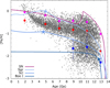 |
Fig. 17 AMRs predicted by chemical evolution models tailored to the solar neighbourhood (magenta line), the Sagittarius dwarf spheroidal galaxy (light blue line), the Sculptor dwarf spheroidal galaxy (medium blue line), and the Boötes I ultra-faint dwarf (dark blue line). The star symbols on top of each curve indicate the ages at which the star formation stops in the dwarf galaxy models. The theoretical AMRs are compared to the distribution of our good-quality TOPoS SG sample in the Age-[Fe/H] plane (grey dots and filled circles). |
6 Comparison with cosmological models for the Local Group assembly
In this Section, we compare our observational data with the cosmological chemical evolution model NEFERTITI (Near-FiEld cosmology: Re-Tracing Invisible Times; Koutsouridou et al. 2023), which is designed to study early galaxy formation processes and the nature of the first (Pop III) stars. The model follows the star formation, chemical enrichment, and assembly histories of galaxies across cosmic time, including the relevant physical and feedback processes. More specifically, it accounts for:
incomplete sampling of the stellar initial mass function (IMF) in galaxies with low SFR (Rossi et al. 2021);
the unknown properties of Pop III stars, which may have different IMFs (Koutsouridou et al. 2024) and may explode as supernovae (SNe) with different energy distribution functions (Koutsouridou et al. 2023);
the transition from Pop III to normal Pop II and Pop I stars Salvadori et al. (2010);
the production and injection of chemical elements, from C to Zn, by different stellar populations, also including SNIa and AGB stars (Koutsouridou et al. 2025);
the inhomogeneous mixing of metals injected by SN-driven outflows into the surrounding intergalactic medium (e.g., Salvadori et al. 2014; Koutsouridou et al. 2026);
the inhomogeneous process of reionisation (Koutsouridou et al. 2026).
We couple NEFERTITI with a suite of ∼30 Caterpillar N-body simulations of the Local Group (Griffen et al. 2016), i.e., the highest-resolution dark-matter-only simulations currently available, which resolve minihalos that hosted the first Pop III stars (e.g., Hirano et al. 2014) and are likely associated with presentday ultra-faint dwarf galaxies (e.g., Salvadori et al. 2015). The NEFERTITI model not only reproduces the present-day mass in stars and gas as well as the metallicities of the Milky Way and the observed metallicity distribution function (MDF) ofGalactic halo stars (see Koutsouridou et al. 2023), but also matches the properties of Milky Way progenitors observed at z ≈ 8 by JWST in the Firefly Sparkle system (Rusta et al. 2024). Therefore, it is an ideal model for studying the assembly of the Milky Way and uncovering the physical origin of the observed stellar AMR.
In Fig. 18, we compare the observed AMR in the Galactic halo with the predictions of NEFERTITI. In the top panel, we show the global AMR for all present-day stars in the Milky Way and its galaxy satellites; in the middle panel, the AMR for stars in the Milky Way only; and in the bottom panel, the AMR for Milky Way stars that formed in situ, i.e., those that, at each epoch, formed exclusively within the most massive dark matter halo in each of the 30 merger histories.
Interestingly, the AMR for Milky Way stars (middle panel) matches the observational findings well. Note that, due to the lack of spatial information for present-day dark matter particles in the Caterpillar simulations, we cannot restrict our analysis to stars predicted to reside specifically in the Galactic stellar halo. As a result, the predicted relations are expected to be broader.
By comparing the different panels, it becomes clear that the low-metallicity AMR can be reproduced only when accreted stars are included in the Milky Way population, i.e., stars that originally formed in low-mass progenitor halos and were subsequently accreted by the Milky Way via merging processes. Although there is no kinematical or orbital characteristic that can unambiguously demonstrate that any given star is the result of an accretion onto the Milky Way, we know that high eccentricity, low or negative angular momentum, and large apocentric distances are clues that point towards accretion. In our sample the stars associated with the low-AMR (see Sect. 4.1) display high eccentricities, 76% of the sample have eccentricity larger than 0.5, the mean eccentricity is 0.66, compared to 0.35 of the complementary sample. The mean angular momentum is −138 kpc km s−1, compared to 1292 kpc km s−1 for the complementary sample. The mean apocentric distance is 14kpc, compared to 10kpc for the complementary sample. Although none of these facts ensures that any of the stars associated with the low-AMR has indeed been accreted, taken collectively, they strongly supportthe notion thatanon-negligible fractionofthem has been accreted. For this reason, the AMR of these accreted stars is similar to that of stars in some of the Milky Way dwarf satellites. Overall, these results indicate that the mostmetal-poor and oldest stars in the Milky Way formed in dwarf galaxy progenitors, thus supporting the scenario proposed to explain the different AMRs discussed in Sect. 4.2.
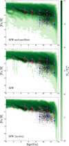 |
Fig. 18 Comparison between the data and the AMR predicted by the NEFERTITI model for stars residing in: the Milky Way and its dwarf satellites (top); the MilkyWay, including stars formed both in situ and in accreted satellites (middle); and the Milky Way, considering only stars formed in situ (bottom). |
7 Discussion and conclusions
In our sample of TOPoS SG stars, we have been able to highlight the existence of three distinct AMRs. In our case, the metallicity of the stars is the fossil record of the metallicity of the gas at the time they were formed. We tentatively associate the mid-AMR and high-AMR with the Galactic discs. Although the thick disc stars mainly follow the mid-AMR there is a non-negligible part that follows the high-AMR. The reverse is true for thin disc stars. We therefore suggest that both discs had some degree of heterogeneity.
The low-AMR can be loosely associated with the Galactic halo, which includes dynamical substructures such as GSE and Sequoia. The fact that a few halo stars are found at metallicities above −1.0 can be understood in terms of the properties of the merging galaxies, which could host relatively metal-rich populations, and may have produced higher metallicity stars in the starburst triggered by the merger.
The fact that the low-AMR is only defined for the three oldest age bins and the large dispersion in metallicities observed in these bins strongly suggest that in this epoch the evolution of the Milky Way was dominated by mergers and that this was rather abruptly terminated about 8 Ga ago. The event changing the evolution from merger-dominated to secular may have been the major merger associated with GSE, but dedicated simulations are necessary to confirm or refute this scenario.
Our proposed scenario is, by and large, supported both by pure chemical evolution models (Sect. 5) and by cosmological models of the Local Group (Sect. 6). We do not seek quantitative agreement between our data and the models, since, as demonstrated by Bonifacio et al. (2021), our sample is extracted from a sample that is highly biased in favour of metal-poor stars and against stars of solar metallicity or higher. Although Bonifacio et al. (2021) corrected for bias for the purpose of the metallicity distribution function, in our case it is not obvious how to do so, since we deal with a subset that has a further selection of the precision of the parallaxes and the colours. We believe it is important that our analysis highlighted the role of mergers in the evolution of the Milky Way up to 8 Ga ago. We are confident that large ongoing wide-field spectroscopic surveys such as WEAVE (Jin et al. 2024), 4MOST (de Jong et al. 2019), and Gaia (Gaia Collaboration 2016), will provide larger and less biased samples for which quantitative comparisons with models will be meaningful. Furthermore, the ESA PLATO mission (Rauer et al. 2025) will provide a large sample of stars with asteroseismic ages, especially for giant stars, which will nicely complement the evolutionary ages, based on SG stars, and will allow us to obtain a clearer view of the AMR in the different components of the Milky Way.
Data availability
Ages and masses for the sample of 8737 stars that are the object of this paper are available at the CDS via https://cdsarc.cds.unistra.fr/viz-bin/cat/J/A+A/711/A260. Other quantities, such as metallicities or actions for these stars are available in the tables associated to the paper Bonifacio et al. (2021) (https://cdsarc.cds.unistra.fr/viz-bin/cat/J/A+A/651/A79) of which the present sample of stars is a sub-set.
Acknowledgements
We are grateful to the anonymous referee for the careful reading of the manuscript and useful suggestions that helped to improve it. We acknowledge the use of the Artificial Intelligence tool Emmy (https://emmy.cnrs.fr) provided by CNRS to perform part of the statistical analysis described in sections two and four. DR acknowledges partial financial support from the project "LEGO – Reconstructing the building blocks of the Galaxy by chemical tagging" (PI: A. Mucciarelli) granted by the Italian MUR through contract PRIN 2022LLP8TK_001. I.K. acknowledges ERC support (grant agreement no. 101117455). L.M. gratefully acknowledges support from ANID-FONDECYT Regular Project no. 1251809. This work has made use of data from the European Space Agency (ESA) mission Gaia (https://www.cosmos.esa.int/gaia), processed by the Gaia Data Processing and Analysis Consortium (DPAC, https://www.cosmos.esa.int/web/gaia/dpac/consortium). Funding for the DPAC has been provided by national institutions, in particular the institutions participating in the Gaia Multilateral Agreement. This paper made use of data from Sloan Digital Sky Survey www.sdss.org.
References
- Akaike, H. 1974, IEEE Trans. Automatic Control, 19, 716 [CrossRef] [Google Scholar]
- Baker, W. M., Tacchella, S., Johnson, B. D., et al. 2025, Nat. Astron., 9, 141 [Google Scholar]
- Barbá, R. H., Minniti, D., Geisler, D., et al. 2019, ApJ, 870, L24 [CrossRef] [Google Scholar]
- Belokurov, V., Erkal, D., Evans, N. W., Koposov, S. E., & Deason, A. J. 2018, MNRAS, 478, 611 [Google Scholar]
- Belokurov, V., Sanders, J. L., Fattahi, A., et al. 2020, MNRAS, 494, 3880 [Google Scholar]
- Bensby, T., Feltzing, S., & Oey, M. S. 2014, A&A, 562, A71 [NASA ADS] [CrossRef] [EDP Sciences] [Google Scholar]
- Bonifacio, P., Sbordone, L., Caffau, E., et al. 2012, A&A, 542, A87 [NASA ADS] [CrossRef] [EDP Sciences] [Google Scholar]
- Bonifacio, P., Monaco, L., Salvadori, S., et al. 2021, A&A, 651, A79 [NASA ADS] [CrossRef] [EDP Sciences] [Google Scholar]
- Bonifacio, P., Caffau, E., Monaco, L., et al. 2024, A&A, 684, A91 [NASA ADS] [CrossRef] [EDP Sciences] [Google Scholar]
- Bonifacio, P., Caffau, E., François, P., & Spite, M. 2025, arXiv e-prints [arXiv:2504.06335] [Google Scholar]
- Caffau, E., Bonifacio, P., Sbordone, L., et al. 2013, A&A, 560, A71 [NASA ADS] [CrossRef] [EDP Sciences] [Google Scholar]
- Caffau, E., Katz, D., Gómez, A., et al. 2024, A&A, 683, A72 [NASA ADS] [CrossRef] [EDP Sciences] [Google Scholar]
- Caffau, E., Katz, D., Bonifacio, P., et al. 2025, Astron. Nachr., 346, e70025 [Google Scholar]
- Casamiquela, L., Reese, D. R., Lebreton, Y., et al. 2024, A&A, 692, A243 [NASA ADS] [CrossRef] [EDP Sciences] [Google Scholar]
- Correnti, M., Gennaro, M., Kalirai, J. S., Cohen, R. E., & Brown, T. M. 2018, ApJ, 864, 147 [NASA ADS] [CrossRef] [Google Scholar]
- Cui, X.-Q., Zhao, Y.-H., Chu, Y.-Q., et al. 2012, Res. Astron. Astrophys., 12, 1197 [Google Scholar]
- de Jong, R. S., Agertz, O., Berbel, A. A., et al. 2019, The Messenger, 175, 3 [NASA ADS] [Google Scholar]
- Ellison, S. L., Patton, D. R., Simard, L., & McConnachie, A. W. 2008, ApJ, 672, L107 [NASA ADS] [CrossRef] [Google Scholar]
- Feuillet, D. K., Sahlholdt, C. L., Feltzing, S., & Casagrande, L. 2021, MNRAS, 508, 1489 [NASA ADS] [CrossRef] [Google Scholar]
- Franchini, M., Morossi, C., Di Marcantonio, P., et al. 2020, ApJ, 888, 55 [NASA ADS] [CrossRef] [Google Scholar]
- Gaia Collaboration (Prusti, T., et al.) 2016, A&A, 595, A1 [NASA ADS] [CrossRef] [EDP Sciences] [Google Scholar]
- Gallart, C., Bernard, E. J., Brook, C. B., et al. 2019, Nat. Astron., 3, 932 [NASA ADS] [CrossRef] [Google Scholar]
- González Hernández, J. I., Bonifacio, P., Caffau, E., et al. 2009, A&A, 505, L13 [Google Scholar]
- Gratton, R. G., Bragaglia, A., Carretta, E., et al. 2003, A&A, 408, 529 [NASA ADS] [CrossRef] [EDP Sciences] [Google Scholar]
- Griffen, B. F., Ji, A. P., Dooley, G. A., et al. 2016, ApJ, 818, 10 [NASA ADS] [CrossRef] [Google Scholar]
- Hammer, F., Wang, J., Mamon, G. A., et al. 2024, MNRAS, 527, 2718 [Google Scholar]
- Haywood, M., Di Matteo, P., Lehnert, M. D., et al. 2018, ApJ, 863, 113 [Google Scholar]
- Helmi, A., Babusiaux, C., Koppelman, H. H., et al. 2018, Nature, 563, 85 [Google Scholar]
- Hidalgo, S. L., Pietrinferni, A., Cassisi, S., et al. 2018, ApJ, 856, 125 [Google Scholar]
- Hirano, S., Hosokawa, T., Yoshida, N., et al. 2014, ApJ, 781, 60 [NASA ADS] [CrossRef] [Google Scholar]
- Jin, S., Trager, S. C., Dalton, G. B., et al. 2024, MNRAS, 530, 2688 [NASA ADS] [CrossRef] [Google Scholar]
- Katz, D., Gómez, A., Caffau, E., et al. 2025, A&A, 704, A294 [NASA ADS] [CrossRef] [EDP Sciences] [Google Scholar]
- Koppelman, H. H., Helmi, A., Massari, D., Price-Whelan, A. M., & Starkenburg, T. K. 2019, A&A, 631, L9 [NASA ADS] [CrossRef] [EDP Sciences] [Google Scholar]
- Koutsouridou, I., Salvadori, S., Skúladóttir, Á., et al. 2023, MNRAS, 525, 190 [NASA ADS] [CrossRef] [Google Scholar]
- Koutsouridou, I., Salvadori, S., & Skúladóttir, Á. 2024, ApJ, 962, L26 [NASA ADS] [CrossRef] [Google Scholar]
- Koutsouridou, I., Skúladóttir, Á., & Salvadori, S. 2025, A&A, 699, A32 [NASA ADS] [CrossRef] [EDP Sciences] [Google Scholar]
- Koutsouridou, I., Salvadori, S., Skúladóttir, Á., et al. 2026, arXiv e-prints [arXiv:2605.00990] [Google Scholar]
- Larson, R. B. 1976, MNRAS, 176, 31 [NASA ADS] [CrossRef] [Google Scholar]
- Lebreton, Y., Goupil, M. J., & Montalbán, J. 2014, in EAS Publications Series, 65, EAS Publications Series, eds. Y. Lebreton, D. Valls-Gabaud, & C. Charbonnel (EDP), 99 [NASA ADS] [CrossRef] [EDP Sciences] [Google Scholar]
- Lebreton, Y., & Reese, D. R. 2020, A&A, 642, A88 [NASA ADS] [CrossRef] [EDP Sciences] [Google Scholar]
- Lilly, S. J., Carollo, C. M., Pipino, A., Renzini, A., & Peng, Y. 2013, ApJ, 772, 119 [NASA ADS] [CrossRef] [Google Scholar]
- Mamajek, E. E., Torres, G., Prsa, A., et al. 2015, IAU 2015 Resolution B2 on Recommended Zero Points for the Absolute and Apparent Bolometric Magnitude Scales [Google Scholar]
- Mannucci, F., Cresci, G., Maiolino, R., Marconi, A., & Gnerucci, A. 2010, MNRAS, 408, 2115 [NASA ADS] [CrossRef] [Google Scholar]
- Massari, D., Zerbinati, C., Fanelli, C., et al. 2026, arXiv e-prints [arXiv:2601.18896] [Google Scholar]
- Michel-Dansac, L., Lambas, D. G., Alonso, M. S., & Tissera, P. 2008, MNRAS, 386, L82 [NASA ADS] [CrossRef] [Google Scholar]
- Mori, A., Di Matteo, P., Salvadori, S., et al. 2025, A&A, submitted [arXiv:2509.13408] [Google Scholar]
- Mucciarelli, A., Bellazzini, M., Ibata, R., et al. 2017, A&A, 605, A46 [NASA ADS] [CrossRef] [EDP Sciences] [Google Scholar]
- Mucciarelli, A., Bonifacio, P., & Lardo, C. 2026, A&A, 705, A134 [NASA ADS] [CrossRef] [EDP Sciences] [Google Scholar]
- Myeong, G. C., Vasiliev, E., Iorio, G., Evans, N. W., & Belokurov, V. 2019, MNRAS, 488, 1235 [Google Scholar]
- Pedregosa, F., Varoquaux, G., Gramfort, A., et al. 2011, J. Mach. Learn. Res., 12, 2825 [Google Scholar]
- Pietrinferni, A., Hidalgo, S., Cassisi, S., et al. 2021, ApJ, 908, 102 [NASA ADS] [CrossRef] [Google Scholar]
- Planck Collaboration VI. 2020, A&A, 641, A6 [NASA ADS] [CrossRef] [EDP Sciences] [Google Scholar]
- Preston, G. W., & Sneden, C. 2000, AJ, 120, 1014 [Google Scholar]
- Preston, G. W., Beers, T. C., & Shectman, S. A. 1994, AJ, 108, 538 [Google Scholar]
- Rauer, H., Aerts, C., Cabrera, J., et al. 2025, Exp. Astron., 59, 26 [Google Scholar]
- Reese, D. R., & Lebreton, Y. 2020, SPInS: Stellar Parameters INferred Systematically, Astrophysics Source Code Library [record ascl:2009.006] [Google Scholar]
- Romano, D., & Starkenburg, E. 2013, MNRAS, 434, 471 [Google Scholar]
- Romano, D., Bellazzini, M., Starkenburg, E., & Leaman, R. 2015, MNRAS, 446, 4220 [CrossRef] [Google Scholar]
- Rossi, M., Romano, D., Mucciarelli, A., et al. 2024, A&A, 691, A284 [NASA ADS] [CrossRef] [EDP Sciences] [Google Scholar]
- Rossi, M., Salvadori, S., & Skúladóttir, Á. 2021, MNRAS, 503, 6026 [NASA ADS] [CrossRef] [Google Scholar]
- Rusta, E., Salvadori, S., Gelli, V., Koutsouridou, I., & Marconi, A. 2024, ApJ, 974, L35 [Google Scholar]
- Salaris, M., Chieffi, A., & Straniero, O. 1993, ApJ, 414, 580 [NASA ADS] [CrossRef] [Google Scholar]
- Salvadori, S., Ferrara, A., Schneider, R., Scannapieco, E., & Kawata, D. 2010, MNRAS, 401, L5 [NASA ADS] [Google Scholar]
- Salvadori, S., Tolstoy, E., Ferrara, A., & Zaroubi, S. 2014, MNRAS, 437, L26 [NASA ADS] [CrossRef] [Google Scholar]
- Salvadori, S., Skúladóttir, Á., & Tolstoy, E. 2015, MNRAS, 454, 1320 [Google Scholar]
- Schwarz, G. 1978, Ann. Statist., 6, 461 [Google Scholar]
- Spitoni, E., Silva Aguirre, V., Matteucci, F., Calura, F., & Grisoni, V. 2019, A&A, 623, A60 [NASA ADS] [CrossRef] [EDP Sciences] [Google Scholar]
- Spitoni, E., Verma, K., Silva Aguirre, V., et al. 2021, A&A, 647, A73 [EDP Sciences] [Google Scholar]
- Torres, S., García-Berro, E., Althaus, L. G., & Camisassa, M. E. 2015, A&A, 581, A90 [NASA ADS] [CrossRef] [EDP Sciences] [Google Scholar]
- VandenBerg, D. A., Brogaard, K., Leaman, R., & Casagrande, L. 2013, ApJ, 775, 134 [Google Scholar]
- Vanni, I., Salvadori, S., Skuladottir, A., Rossi, M., & Koutsouridou, I. 2023, MNRAS, 526, 2620 [NASA ADS] [CrossRef] [Google Scholar]
- Vasiliev, E., & Baumgardt, H. 2021, MNRAS, 505, 5978 [NASA ADS] [CrossRef] [Google Scholar]
- Villanova, S., Monaco, L., Geisler, D., et al. 2019, ApJ, 882, 174 [NASA ADS] [CrossRef] [Google Scholar]
- Wang, L., De Lucia, G., Fontanot, F., & Hirschmann, M. 2019, MNRAS, 482, 4454 [Google Scholar]
- Wang, J., Hammer, F., Yang, Y., et al. 2024, MNRAS, 527, 7144 [Google Scholar]
- Yang, Y., Caffau, E., Bonifacio, P., et al. 2024, A&A, 691, A363 [NASA ADS] [CrossRef] [EDP Sciences] [Google Scholar]
- York, D. G., Adelman, J., Anderson, J. E., Jr. et al. 2000, AJ, 120, 1579 [NASA ADS] [CrossRef] [Google Scholar]
We adopt the definitions of metal-poor (MP), very metal-poor (VMP), extremely metal-poor (EMP), and ultra metal-poor (UMP) stars from Bonifacio et al. (2025), Table 1.
Appendix A Estimating luminosities and associated errors
The relations between surface gravity g of a star of mass M and radius R, its luminosity L and effective temperature Teff are summarised in equations A.1 − A.3.
 (A.1)
(A.1)
 (A.2)
(A.2)
 (A.3)
(A.3)
In the sample of Bonifacio et al. (2021) the surface gravity is provided, this has been obtained assuming a stellar mass of 0.8M⊙. To determine ages we prefer to use the surface luminosity. In order to derive the stellar luminosity we re-arrange equation A.3 to yield:
 (A.4)
(A.4)
We used this equation assuming a mass of 0.8M⊙, that is consistent with the log g provided in (Bonifacio et al. 2021). Taking into account that the relation between luminosities and bolometric magnitudes is
 (A.5)
(A.5)
Where μ denotes absolute magnitudes, and recalling that the absolute bolometric magnitude of the Sun is 4.74 (Mamajek et al. 2015) and introducing the parallax of the star ϖ, and recalling that
 (A.6)
(A.6)
where G is the Gaia G magnitude and Gc is the corresponding bolometric correction, one can also write
 (A.7)
(A.7)
Equation A.7 is useful because it allows to establish that error on the luminosity depends only on the error on G and on the parallax in practice
 (A.8)
(A.8)
We used equation A.4 to compute  for all the stars in the "good parallax" sample of Bonifacio et al. (2021). Equation A.8 was used to estimate the errors on logarithmic luminosity. As error in G magnitude we used the estimate provided by CDS, that besides the photon-noise error includes a floor of Gf = 0.0027553202 mag3, in practice:
![Mathematical equation: $\Delta G\sqrt {{{\left[ {\left( {{{ - 2.5} \over {{\rm{ln}}\left( {10} \right)}}} \right)\left( {{{\Delta \left( {{\rm{Flux}}} \right)} \over {{\rm{Flux}}}}} \right)} \right]}^2} + G_f^2} $](/articles/aa/full_html/2026/07/aa60236-26/aa60236-26-eq13.png) (A.9)
(A.9)
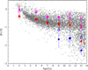 |
Fig. B.1 Same as Fig. 8, except that the ages are derived without any prior, the open circles identify the peaks in any age bin, while the filled circles show the peaks derived from the dataset where ages were derived using a flat prior imposing ages to be in the interval from zero to 13.8 Ga. The colour coding is the same as in Fig. 8. |
Appendix B Using ages derived without any prior
In Fig. B.1 we show the age-metallicity relation using the ages derived without any prior, we shall refer to this sample as the "no-prior" sample. We retained only the stars for which SPInS derived an age smaller than the age of the Universe, this reduces the sample to 60% of the original sample (5 273 stars). We analysed the no-prior sample in the same way as described in Sect.4.1, the position of the peaks is denoted by open circles, while the filled circles are the position of the peaks in Fig. 8. The most noticeable differences are in the oldest age bin, where the peaks in the no-prior sample appear systematically at higher metallicities even by 1 dex. The differences become smaller and smaller as we move to the younger metallicity bins. We conclude that the general morphology of the age-metallicity relations does not depend on whether one applies a prior on age or not in the age determination. We stress that our sample, whatever the hypothesis made on the age determination, is biased in favour of metal-poor stars as discussed in Bonifacio et al. (2021). In order to determine precisely the position of the peaks, especially in the oldest age bins, we need an unbiased sample.
All Tables
Percentage of stars classified as thin disc, thick disc, and halo along with each of the three AMRs.
All Figures
|
Fig. 1 Colour magnitude diagram of the TOPoS stars with those we analyse as SGs in blue, the others in red. To guide the eye we superimpose three BaSTI (Pietrinferni et al. 2021) isochrones with ages 4, 8, and 12 Ga and [Fe/H]=−0.4 (green) and −2.5 (grey). |
| In the text | |
|
Fig. 2 Hertzsprung-Russell diagram for the SG stars of NGC6397 that we used to estimate its age. Three BASTI isochrones of 12, 13, and 14 Ga and metallicity −2.0 are shown for reference. |
| In the text | |
|
Fig. 3 AMR from our sample assuming a prior on age (green dots), our sample without any prior (red dots), and the sample of Casamiquela et al. (2024) (blue dots). Note that there are red dots and blue dots below the green dots. |
| In the text | |
|
Fig. 4 Metallicity histogram of our sample (blue), compared with the LRS sample of Casamiquela et al. (2024) (green). The two histograms have been normalised by the number of stars in each sample. |
| In the text | |
|
Fig. 5 Toomre diagram that we used to select thin disc and thick disc stars. |
| In the text | |
 |
Fig. 6 Same as Fig. 5 but for the whole sample of SGs, without any cut on the error in luminosity. |
| In the text | |
|
Fig. 7 Dynamically selected populations in the angular momentum-energy plane. The grey points are all the stars that cannot be classified as disc (thick or thin), GSE, or Sequoia. The grey points plus Sequoia, plus GSE, is what can generically be called halo. The units for energy are 103 × km2 s2 (actually it is a specific energy, or energy per unit mass) and 103 × kpc km s−1 for the angular momentum. |
| In the text | |
|
Fig. 8 AMR as defined from our dataset. The data are divided into six age bins, and for each bin we show the points corresponding to the centre of the bin and to the metallicity of the peaks. The vertical bars correspond to the FWHM of a Gaussian to each peak. The blue dots correspond to the low-AMR, the red dots to the mid-AMR, and the purple points to the high-AMR. |
| In the text | |
|
Fig. 9 Histogram of the metallicities in the age bin 10–12 Ga. The fitted Gaussians are shown both individually (blue, red, magenta lines) and summed (black line). |
| In the text | |
|
Fig. 10 As Fig. 8, but now only the stars classified as GSE are shown. The meaning of the colours of the dots is the same as in Fig. 8. |
| In the text | |
|
Fig. 11 As Fig. 8, but now only the stars classified as thick disc are shown. The meaning of the colours of the dots is the same as in Fig. 8. |
| In the text | |
|
Fig. 12 As Fig. 8, but now only the stars classified as thin disc are shown. The meaning of the colours of the dots is the same as in Fig. 8. |
| In the text | |
|
Fig. 13 As Fig. 8, but now only the stars classified as Sequoia are shown. The meaning of the colours of the dots is the same as in Fig. 8. |
| In the text | |
|
Fig. 14 As Fig. 8, but now only the stars classified as halo are shown. The meaning of the colours of the dots is the same as in Fig. 8. |
| In the text | |
|
Fig. 15 Contour plot of the two extreme age bins (youngest and oldest) in the R, |z| plane. |
| In the text | |
|
Fig. 16 Stars in our sample that classify as blue metal-poor according to the criteria of Preston et al. (1994). |
| In the text | |
|
Fig. 17 AMRs predicted by chemical evolution models tailored to the solar neighbourhood (magenta line), the Sagittarius dwarf spheroidal galaxy (light blue line), the Sculptor dwarf spheroidal galaxy (medium blue line), and the Boötes I ultra-faint dwarf (dark blue line). The star symbols on top of each curve indicate the ages at which the star formation stops in the dwarf galaxy models. The theoretical AMRs are compared to the distribution of our good-quality TOPoS SG sample in the Age-[Fe/H] plane (grey dots and filled circles). |
| In the text | |
|
Fig. 18 Comparison between the data and the AMR predicted by the NEFERTITI model for stars residing in: the Milky Way and its dwarf satellites (top); the MilkyWay, including stars formed both in situ and in accreted satellites (middle); and the Milky Way, considering only stars formed in situ (bottom). |
| In the text | |
|
Fig. B.1 Same as Fig. 8, except that the ages are derived without any prior, the open circles identify the peaks in any age bin, while the filled circles show the peaks derived from the dataset where ages were derived using a flat prior imposing ages to be in the interval from zero to 13.8 Ga. The colour coding is the same as in Fig. 8. |
| In the text | |
Current usage metrics show cumulative count of Article Views (full-text article views including HTML views, PDF and ePub downloads, according to the available data) and Abstracts Views on Vision4Press platform.
Data correspond to usage on the plateform after 2015. The current usage metrics is available 48-96 hours after online publication and is updated daily on week days.
Initial download of the metrics may take a while.