


| Issue |
A&A
Volume 711, July 2026
|
|
|---|---|---|
| Article Number | A217 | |
| Number of page(s) | 15 | |
| Section | Stellar structure and evolution | |
| DOI | https://doi.org/10.1051/0004-6361/202660086 | |
| Published online | 16 July 2026 | |
Identifying hot subdwarf binaries with multimodal deep learning
Based on Gaia and SDSS data
1
School of Mathematics and Statistics, Shandong University, Weihai, 264209 Shandong, People’s Republic of China
2
School of Space Science and Technology, Shandong University, Weihai, 264209 Shandong, China
3
School of Airspace Science and Engineering, Shandong University, Weihai, 264209 Shandong, China
4
Shandong Key Laboratory of Intelligent Electronic Packaging Testing and Application, Shandong University, Weihai, 264209 Shandong, China
★ Corresponding author: This email address is being protected from spambots. You need JavaScript enabled to view it.
Received:
27
March
2026
Accepted:
23
May
2026
Abstract
Context. Hot subdwarf stars are important tracers of stellar structure and evolution, while their binary systems provide key constraints on their formation channels. Nevertheless, the number of confirmed hot subdwarf binaries is still limited.
Aims. We aim to identify hot subdwarf binaries efficiently and reliably in large candidate samples by combining heterogeneous observational information.
Methods. We developed a two-stage classification framework. A Bayesian neural network was first used to perform preliminary classification and uncertainty quantification from Gaia photometric and astrometric data. We then constructed a multimodal deep learning model, HsdB-FusionNet, which combines Gaia photometric and astrometric features with SDSS spectra through a cross-attention mechanism. We applied this framework to a catalog of 61 585 hot subdwarf candidates. The resulting candidates were further examined through spectral energy distribution fitting, and atmospheric parameters were derived for high-quality systems.
Results. We identified 1369 hot subdwarf binary candidates from the parent sample. Among them, 1057 objects were strongly supported as binaries by spectral energy distribution fitting. Atmospheric parameters were obtained for 579 high-quality binary systems. The interpretability analysis further indicates that the model decisions are consistent with known physical priors.
Conclusions. This work provides a substantially enlarged sample of hot subdwarf binary candidates and demonstrates the potential of multimodal deep learning for binary identification. The released catalog offers a useful basis for future studies on the formation and evolution of hot subdwarf binaries.
Key words: methods: data analysis / techniques: photometric / techniques: spectroscopic / binaries: general / subdwarfs
© The Authors 2026
 Open Access article, published by EDP Sciences, under the terms of the Creative Commons Attribution License (https://creativecommons.org/licenses/by/4.0), which permits unrestricted use, distribution, and reproduction in any medium, provided the original work is properly cited.
This article is published in open access under the Subscribe to Open model. This email address is being protected from spambots. You need JavaScript enabled to view it. to support open access publication.
1. Introduction
Hot subdwarfs represent a typical class of evolved stars, commonly regarded as the exposed helium-burning cores of red giants that have lost their hydrogen-rich envelopes through substantial mass loss (Heber 2009, 2016). Characterized by high temperatures and low luminosities, their surface temperatures typically range from 20 000 to 70 000 K, and their luminosities are lower than those of main-sequence (MS) stars. They are located near the blue end of the horizontal branch in the Hertzsprung–Russell (HR) diagram. Based on their spectral characteristics, hot subdwarfs are further classified into B (sdB) and O (sdO) subtypes (Drilling et al. 2013).
Hot subdwarfs are found across all major Galactic populations and serve as important tracers for Galactic chemical evolution, stellar population structure, and late-stage stellar evolution (Vasishta 2025). Moreover, they are considered key contributors to the far-ultraviolet (FUV) background radiation (Han et al. 2010). For instance, sdB stars are widely regarded as the primary sources responsible for the ultraviolet upturn observed in elliptical galaxies (O’Connell 1999). Observationally, hot subdwarfs are characterized by low masses (∼0.47 M⊙), extremely thin hydrogen envelopes (∼0.01 M⊙), and high surface gravities (5.0 ≲ log g ≲ 6.5). Such a tenuous hydrogen layer directly indicates that their progenitors experienced substantial mass loss during previous evolutionary stages. However, the physical mechanisms driving such extreme mass-loss episodes remain uncertain, representing one of the central scientific questions in the study of hot subdwarfs (Heber 2009; Ostrowski et al. 2021).
Binary evolution is now widely recognized as the dominant formation channel for hot subdwarf stars. Although single-star channels were proposed in earlier studies, they fail to account for the efficiency of envelope stripping and the observed distribution of hot subdwarfs (Xiong et al. 2017). In contrast, binary evolution models better reproduce their observed properties, including mass and envelope structure (Taam & Sandquist 2000; Zhang & Jeffery 2012). Three main channels have been proposed: the common envelope (CE) ejection channel, where unstable mass transfer leads to envelope ejection and produces compact sdB binaries with white dwarf (WD) or MS companions and orbital periods of just a few hours (Han et al. 2003); the stable Roche-lobe overflow (RLOF) channel, yielding wide sdB binaries with periods up to thousands of days (Han et al. 2003); and the merger of two low-mass helium white dwarfs (He WDs), resulting in a single sdB star (Iben & Tutukov 1986). Extensive observational evidence supports the significance of binary evolution channels in the formation of hot subdwarfs. For example, more than two-thirds of observed sdB stars are found in close binary systems – a binary fraction significantly higher than that of normal stellar populations (Maxted et al. 2001; Lisker et al. 2005). Kupfer et al. (2020) reported a Roche-lobe-filling sdOB binary with a WD companion and an orbital period as short as 56 min, providing direct evidence that hot subdwarfs can undergo dramatic mass transfer and orbital evolution during their formation. Therefore, a systematic analysis of hot subdwarf binaries, including companion types and orbital parameters, not only helps characterize their current physical state but also provides critical clues for reconstructing their evolutionary pathways.
In currently studied hot subdwarf binary systems, the companion types exhibit great diversity. In short-period systems (typically 0.1–10 days), the companions are usually WDs, low-mass MS stars (M or K types), or brown dwarfs (BDs). These systems are generally thought to originate from the CE evolution channel (Geier et al. 2011). In contrast, wide-orbit systems with orbital periods exceeding 100 days are generally formed via stable RLOF or wind-driven mass-loss mechanisms (Han et al. 2002; Vos et al. 2018). In such systems, hot subdwarfs are typically paired with F- or G-type MS stars, forming composite spectrum binaries. Early studies (Thejll et al. 1995; Ulla & Thejll 1998) pointed out that some of these systems exhibit significant infrared (IR) excess in the near-IR JHK bands, primarily due to the contribution from A–K-type MS companions. Several advanced spectral decomposition techniques, such as XTGRID and GSSP, have been widely applied to the analysis of composite systems, confirming multiple wide sdB binaries with G- or K-type companions (Németh et al. 2021; Molina et al. 2022).
Time-domain observations and asteroseismology offer crucial tools for identifying hot subdwarf binary systems. Many sdB stars are observed as pulsating variables, exhibiting non-radial pressure modes (V361 Hya type) and gravity modes (V1093 Her type), with some stars exhibiting hybrid pressure and gravity modes (Kilkenny et al. 1997; Fontaine et al. 2003; Reed et al. 2010). Asteroseismic analysis of these pulsations enables precise determination of their internal structure, envelope mass, and evolutionary state, which are key parameters for inferring their formation channels and potential binarity (Charpinet et al. 2005; Østensen et al. 2010). Moreover, high-precision time-domain surveys such as TESS and Kepler have significantly advanced the study of photometric variability in hot subdwarfs, revealing numerous binary systems exhibiting signatures of reflection effects, ellipsoidal variations, and eclipses (Schaffenroth et al. 2023). These periodic photometric signals provide robust evidence for the presence of compact companions and serve as one of the most effective methods for distinguishing between single and binary systems. By modeling the light curve’s period, amplitude, and phase, and combining them with spectroscopic dynamical analyses, researchers can further infer the companion’s mass and orbital parameters (Uzundag et al. 2024; Ranaivomanana et al. 2025). Ongoing photometric and dynamical studies are enhancing our understanding of hot subdwarf binaries and underscore the need for improved classification frameworks.
The initial identification of hot subdwarfs dates back to the 1950s. Humason & Zwicky (1947) were the first to discover these subluminous blue objects during a photometric survey of the North Galactic Pole. Systematic large-scale search efforts began in the 1980s, with the most representative among them being the Palomar-Green (PG) survey and the Edinburgh-Cape (EC) survey. Based on these data, Kilkenny et al. (1988) published the first catalog of hot subdwarfs, which included 1225 objects. The release of Gaia DR2 (Babusiaux et al. 2018) opened new avenues for the identification of hot subdwarf stars. Gaia provides highly accurate measurements of colors, absolute magnitudes, and proper motions, enabling researchers to define the region of hot subdwarfs in the HR diagram. Lei et al. (2018, 2019, 2020, 2023) and Luo et al. (2019, 2021) initially selected candidates based on Gaia photometry and their locations in the HR diagram and then cross-matched these sources with LAMOST spectra. Hot subdwarfs were subsequently confirmed through spectral template matching. In 2022, following the release of Gaia EDR3, Culpan et al. (2022) compiled previous efforts and published the largest catalog of hot subdwarfs to date, increasing the number of known hot subdwarfs to 6616 and expanding the catalog of candidates to 61 585. In the search for hot subdwarf binaries, traditional methods rely on color selection criteria, multiband spectral energy distribution (SED) fitting, and IR excess diagnostics (Vos et al. 2018; Kupfer et al. 2020). Solano et al. (2022) developed an SED-based approach using the VOSA Virtual Observatory tool (Bayo et al. 2008), supported by the SVO Filter Profile Service (Rodrigo & Solano 2020), to identify composite systems with IR excess and to estimate their physical properties.
In recent years, the release of large-scale photometric and spectroscopic data from various sky surveys has posed challenges to traditional search methods, which are inefficient and lack scalability when dealing with massive datasets. The development of machine learning has provided new opportunities for the efficient processing of astronomical data. Researchers such as Bu et al. (2017, 2019), Tan et al. (2022), and Cheng et al. (2024) have applied methods including hierarchical extreme learning machines (HELMs), convolutional neural networks (CNNs), and support vector machines (SVMs) to directly search for hot subdwarf stars from spectral data. Graph neural networks have also been utilized to identify candidates from Gaia and Pan-STARRS photometry (Liu et al. 2024). Other researchers have used neural networks to classify candidates directly from SDSS photometric images (Wu et al. 2025; Zhang et al. 2025). For hot subdwarf binaries, recent studies have begun to apply machine-learning techniques directly to binary classification. Vázquez et al. (2024) combined Gaia DR3 color–magnitude information with Gaia BP/RP spectra and used SVM, SOM, and CNN methods to distinguish single and composite hot subdwarf systems. Ambrosch et al. (2026) further extended this Gaia-XP-based strategy to a larger sample of approximately 20 000 hot subdwarf candidates and investigated the connection between binarity and Gaia-based diagnostic features. A related LAMOST-based study developed a Bayesian spectral-learning framework to identify hot subdwarf binaries from low-resolution LAMOST spectra (Yang et al. 2026). These studies demonstrate the increasing potential of machine-learning methods for hot subdwarf binary searches.
Compared to the increasingly mature techniques for automatically identifying single hot subdwarfs, the identification of binary systems still faces significant challenges. On the one hand, systematic searches targeting hot subdwarf binaries are still relatively scarce, resulting in limited observational samples that restrict us from further understanding their formation and evolutionary pathways. On the other hand, most existing classification models rely on single-modality data, typically photometric or spectroscopic data, thus failing to fully exploit the complementary nature of these datasets. For instance, spectroscopic features such as double-lined profiles, Doppler shifts, and IR excess are key indicators of binarity, while Gaia-based colors, magnitudes, proper motions, and astrometric diagnostics also correlate with binary systems. Furthermore, the scarcity of confirmed samples as well as missing or incomplete observations necessitate the development of robust classification models capable of handling data incompleteness effectively.
In light of the above context, we propose a novel framework for identifying and classifying hot subdwarf systems by integrating deep learning with multisource observational data. Specifically, we combined photometric and astrometric data from Gaia DR3 with spectroscopic observations from SDSS to construct a unified multimodal model. Before performing data fusion, we employed a Bayesian neural network (BNN) combined with a masking strategy to address the issue of missing photometric observations in part of the sample. This approach allowed us to mitigate the effect of incomplete data while providing uncertainty-aware classification. Subsequently, a cross-attention mechanism was introduced to integrate heterogeneous features, thereby significantly improving the identification accuracy. To enhance the interpretability and scientific reliability of the model, we further incorporated explainable artificial intelligence techniques to interpret decision-making patterns. Finally, we validated selected binary candidates through SED fitting using the VOSA tool.
This paper is organized as follows. Section 2 introduces the catalogs used and the associated photometric and spectroscopic data. Section 3 presents our binary identification framework, including a Bayesian classification model and the multimodal HsdB-FusionNet. Section 4 reports the classification results, evaluates model interpretability through feature attribution, and compares performance under different data settings. Section 5 extends the application to a larger dataset and performs physical confirmation of the binary candidates. Section 6 summarizes our findings and outlines future directions.
2. Data
Culpan et al. (2022) compiled a catalog of 6616 confirmed hot subdwarfs and 61 585 hot subdwarf candidates by combining photometric and astrometric data from Gaia EDR3 with spectroscopic data from large-scale surveys such as LAMOST and SDSS. Based on the color–magnitude diagram, they proposed an approximate boundary between single and binary hot subdwarfs: single stars primarily occupy the region with GBP − GRP ≤ 0.0, while binaries with cooler companions tend to appear in redder regions. They found that the renormalized unit weight error (RUWE) and astrometric excess noise are useful Gaia astrometric diagnostics for identifying potential unresolved binaries. RUWE measures the goodness of fit of the Gaia single-source astrometric solution, while astrometric excess noise quantifies additional residual scatter beyond the formal astrometric uncertainties. Elevated values may indicate unresolved binarity, orbital or photocenter motion, or other departures from the single-source astrometric model. Meanwhile, binary systems often exhibit spectral features such as double lines, Doppler shifts, and IR excess. To achieve more reliable classification, this work combines photometric, astrometric, and spectroscopic data for joint analysis. Specifically, we used five features from Gaia DR3, including GBP − GRP color, parallax, absolute magnitude, RUWE, and astrometric excess noise, as well as spectroscopic data from SDSS DR18 to classify hot subdwarf binaries.
The binary and single-star labels used in this study were derived through a comprehensive review and synthesis of multiple prior works, including Kupfer et al. (2015), Geier et al. (2017), Vos et al. (2018), Pelisoli et al. (2020), Solano et al. (2022), Culpan et al. (2022), and Schaffenroth et al. (2023). The initial catalog contained 6616 hot subdwarf entries. After removing duplicated sources, we obtained 6575 unique hot subdwarf objects for label construction.
For each object, we collected the available binary and single-star classifications from eight literature-based labels. Since the number of available labels varied among objects, we used a confidence-based aggregation procedure rather than a simple majority vote. Let N be the number of available labels, S the number of single-star labels, and B the number of binary labels. In the initial voting step, for objects with N ≤ 4, a single-star label was assigned only when all labels were single, whereas a binary label was assigned when B ≥ 3 and B > S. For objects with N ≥ 5, a single-star label was assigned when S ≥ 4 and B ≤ 1, whereas a binary label was assigned when B ≥ 3 and B > S. The asymmetric criterion reflects the fact that binary labels usually correspond to positive observational evidence for binarity, whereas a single-star label may simply indicate that no binary signature was detected in a given dataset. Weak, borderline, or inconsistent cases were then manually inspected. Objects were excluded as conflicting or ambiguous if the available labels and manual inspection did not provide sufficiently reliable evidence for either class.
Following this procedure, we retained 4878 high-confidence labeled objects, including 3851 single stars and 1027 binaries, while 1697 objects were excluded because of insufficient or conflicting label information. This labeling strategy is analogous to expert aggregation in weakly supervised learning and was adopted to improve the reliability of the training labels.
We then cross-matched the 6575 unique confirmed hot subdwarfs with Gaia DR3 and SDSS DR18. The Gaia DR3 cross-match did not remove any of these objects; when individual Gaia features were unavailable, the corresponding missing entries were retained and handled through the masking strategy described in Sect. 3.1.2. In contrast, SDSS DR18 spectra were available for 2032 entries in the original catalog, corresponding to 2019 unique confirmed hot subdwarf objects after duplicate removal. Among these SDSS-matched objects, 1548 also had high-confidence binary or single-star labels and were used for the multimodal Gaia–SDSS training and evaluation.
After constructing and validating the classification model, we further applied it to the catalog of 61 585 hot subdwarf candidates compiled by Culpan et al. (2022). Gaia photometric and astrometric information was available for these candidates, while SDSS DR18 spectra were available for 3230 candidates. These 3230 candidates were used for the subsequent multimodal classification, and the resulting binary candidates were subjected to additional validation and verification.
3. Methods
To effectively leverage multisource observational data while balancing large-sample coverage and classification accuracy, we designed a two-stage classification framework. In the first stage, a BNN model was developed using photometric and astrometric data from Gaia DR3 to perform preliminary classification of hot subdwarf binaries. Given the limited availability of high-quality spectroscopic data, this model aims to enable rapid screening and probability estimation of binary systems across a large number of candidates, thereby enabling the identification of more potential binary systems.
Building on this foundation, we further developed a multimodal deep learning model, HsdB-FusionNet, to enhance classification accuracy and reliability. This model integrates photometric and astrometric data from Gaia with spectroscopic data from SDSS into a unified feature space, thereby overcoming the limitations of single-modality approaches in previous studies. Through deep representation learning, the model effectively captures binary-related features across different data types, enabling more refined identification and confidence estimation of hot subdwarf binary systems.
3.1. Construction of BNN classification model
In the classification of single and binary hot subdwarf systems, traditional neural networks can provide classification outcomes but lack the ability to quantify the reliability of their predictions. This ability is particularly critical for hot subdwarfs located near the boundary between single and binary classifications, where it is often difficult to make definitive distinctions based solely on photometric features such as the color–magnitude diagram.
In this context, incorporating BNNs is particularly meaningful (Kononenko 1989; Mullachery et al. 2018; Jospin et al. 2022). Unlike traditional neural networks that produce deterministic predictions, BNNs yield full posterior probability distributions, enabling principled uncertainty quantification. This is especially valuable in the classification of hot subdwarfs, where observational limitations, intrinsic astrophysical complexity, and the propagation of measurement errors contribute to significant uncertainty. The Bayesian framework naturally accommodates these uncertainties and provides predicted distributions rather than deterministic labels.
3.1.1. Model framework and variational inference
The BNN treats the network weights as random variables and models the parameter uncertainty via posterior distributions. This approach is particularly suitable for addressing observational errors and sample uncertainties. Given a newly observed hot subdwarf star x∗, the BNN estimates the probability of it being a binary system by marginalizing over all possible weight configurations:
 (1)
(1)
where y∗ denotes the model prediction for input x∗, ω represents the network parameters, and p(y∗ ∣ x∗,ω) is the likelihood given a specific parameter configuration, and p(ω ∣ D) is the posterior parameter distribution given the training data 𝒟.
Since the above integral is generally intractable, we adopt variational inference to approximate the posterior using a learnable distribution qθ(ω)≈p(ω ∣ 𝒟), by maximizing the evidence lower bound (ELBO) (Graves 2011; Sun et al. 2019):
![Mathematical equation: $$ \begin{aligned} \mathrm{ELBO}(\theta ) = \mathbb{E} _{q_{\theta }(\omega )} \left[ \log p(D \mid \omega ) \right] - \mathrm{KL} \left( q_{\theta }(\omega ) \,\Vert \, p(\omega ) \right). \end{aligned} $$](/articles/aa/full_html/2026/07/aa60086-26/aa60086-26-eq2.gif) (2)
(2)
Here, p(𝒟 ∣ ω) is the likelihood of the training data given parameters ω, and p(ω) is the prior.
To enable efficient gradient-based optimization, we adopted the Flipout technique for decorrelated parameter sampling (Wen et al. 2018). Each parameter matrix was parameterized by its mean μw and standard deviation σw, from which pseudo-random samples were drawn as
 (3)
(3)
where ε ∼ 𝒩(0,I) is a standard normal random tensor, and r and S are random sign vectors that take values of −1 or 1, used to reduce intra-mini-batch correlations. During training, we used the KL divergence as the regularization term and applied a shrinkage coefficient β = 0.1 to control model complexity and mitigate overfitting. The overall architecture of the BNN model is shown in Fig. 1.
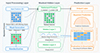 |
Fig. 1. Architecture of the BNN. The model consists of three main components. (1) Input processing layer: The input feature matrix X, possibly containing missing values, is accompanied by a binary mask indicating valid entries (features ≠ −999), followed by standardization. (2) Masked hidden layer: The standardized features are combined with the mask via the Hadamard product to obtain masked features, which are processed through two hidden layers with Bayesian weight distributions and dropout regularization. (3) Prediction layer: The output layer produces a Bayesian predictive distribution, evaluated through five-fold cross-validation. Model performance was assessed using accuracy, confusion matrices, and uncertainty quantification. |
3.1.2. Feature preprocessing
To capture differences between single and binary systems in terms of photometric and astrometric properties, we included five features from Gaia DR3: GMAG, color index (GBP − GRP), Plx, RUWE, and astrometric excess noise. Here, GMAG and GBP − GRP describe the photometric properties of the source, Plx provides astrometric distance information, and RUWE and astrometric excess noise are Gaia astrometric diagnostics.
However, due to the incomplete coverage of photometric and astrometric measurements in certain samples, some missing feature values were encoded as the default placeholder value −999. Considering the limited number of known binary hot subdwarfs, we did not discard samples with missing entries. Instead, we adopted a mask-based strategy to retain maximal sample diversity while preserving the available observational information (Guo et al. 2019).
Specifically, we defined a binary mask matrix M ∈ {0,1}n×d to indicate the presence or absence of valid features and applied it to the original feature matrix X using a Hadamard product:
 (4)
(4)
where X denotes the original feature matrix, and μ and σ are the mean and standard deviation vectors computed over non-missing entries for each feature dimension, respectively. The operator ⊙ represents element-wise (Hadamard) multiplication. This approach ensures that the model learns valid feature representations only from observed values, thereby avoiding overfitting to missing-value placeholders or noise.
3.1.3. Loss function and uncertainty quantification
Hot subdwarfs exhibit significant class imbalance between single and binary systems, along with incomplete photometric and astrometric measurements. These factors result in biased representations and compromised discriminative power in classification. To address these issues, we propose a two-level sample reweighting scheme to enhance the model’s ability to identify binaries and to increase robustness against missing data.
First, to account for feature completeness across samples, we defined a per-sample feature quality weight wifeat, which is proportional to the fraction of valid features in the i-th sample:
 (5)
(5)
Second, to address class imbalance between singles and binaries, we adopted a dynamic class-weighting mechanism. Let  denote the model’s current average prediction probability for the binary class. The adjusted sample weight w′i is defined as
 (6)
(6)
This dynamic scheme increases the importance of binary samples that are currently under-recognized by the model (i.e., with small  ), encouraging the model to focus more on identifying rare or hard-to-classify binaries. Conversely, as the model improves and
  , the class weights for binary and single stars converge, thereby avoiding overfitting. The final loss function is the weighted binary cross-entropy:
![Mathematical equation: $$ \begin{aligned} L_{\mathrm{CE} } = - \sum _{i = 1}^{n} w^{\prime } \left[ y_i \log (\hat{y}_i) + (1 - y_i) \log (1 - \hat{y}_i) \right] . \end{aligned} $$](/articles/aa/full_html/2026/07/aa60086-26/aa60086-26-eq10.gif) (7)
(7)
During the prediction phase, we performed 1000 posterior weight samplings to obtain the predictive distribution of each sample i, denoted as  , where
  is the predicted probability for sample i under the k-th sampled weight configuration. Based on this distribution, we computed the mean and uncertainty of the predictive probability:
 (8)
(8)
where  denotes the final predictive probability, and σi represents the predictive uncertainty. A smaller σi indicates greater confidence in the model’s prediction for sample i. To assess the effectiveness of this uncertainty quantification, we further analyzed the correlation between predictive accuracy and uncertainty. Specifically, we computed the Pearson correlation coefficient between prediction correctness and uncertainty. Finally, we adopted K-fold cross-validation to comprehensively assess model generalization and verify the reliability of uncertainty estimation.
3.2. Fusion model: HsdB-FusionNet
To improve the reliability of binary classification using limited photometric and astrometric information, we propose a multimodal fusion classification model, HsdB-FusionNet, based on the cross-attention mechanism and the Bayesian framework established in Sect. 3.1. The model integrates photometric and astrometric data from Gaia and spectroscopic data from SDSS. HsdB-FusionNet consists of three core modules: the encoder module, the feature fusion module, and the decoder module. The overall architecture of HsdB-FusionNet, including the spectral feature extractor (SFE) and the multimodal fusion module, is shown in Fig. 2.
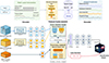 |
Fig. 2. Architecture of the HsdB-FusionNet. (a) Top: simplified pipeline of the SFE. The spectrum (∼3800 dims) is processed by multi-scale 1D convolutions (kernels k = {3, 9, 27}) and residual blocks to capture local and cross-scale patterns. Their features are fused through a main path and a line path, and the decoder predicts the reconstructed spectrum together with its continuum and line components. (b) Bottom: overall architecture of HsdB-FusionNet. The network consumes three inputs – SFE spectral features S, BNN embeddings B, and BNN auxiliary uncertainty (σ, p), which pass through spectral-wise and BNN-wise attention streams and fully connected layers. The fusion module combines a cross-attention unit (S → B, B → S) with an uncertainty-weighted unit using Sigmoid scaling (gated by σ). The concatenated representation is fed to multilayer perceptron (MLP) heads and a classifier to output the hot-subdwarf single and binary probability. |
The encoder module extracts preliminary representations from photometric and spectral inputs. For the photometric stream, we encoded features such as stellar brightness and proper motion, while for spectroscopy, we extracted 128D continuous representations from the raw spectra. The feature fusion module employs a cross-attention mechanism to deeply integrate complementary information from different modalities. Moreover, the decoder processes the fused representation to yield the final binary classification output. The model also supports spectral reconstruction to verify the completeness of spectral encoding.
3.2.1. Feature encoder
In the feature extraction stage, HsdB-FusionNet constructs feature representations by integrating photometric, astrometric, and spectroscopic data. For the photometric and astrometric inputs, we leveraged the intermediate layers of a pretrained BNN as feature encoders, obtaining a 32D embedding that captures critical brightness and motion information. For spectral data, we specifically designed a spectroscopic encoder that converts raw spectra into a 128D continuous feature vector.
To effectively capture the distinctive spectroscopic characteristics of hot subdwarf binaries and singles, we designed a novel encoder-decoder architecture. An effective spectral feature should be capable of reconstructing the original spectrum. The encoder compresses the raw 3800D spectral vector into a 128D embedding and enhances feature expressiveness through task-oriented reconstruction.
The encoder employs multi-scale convolutional layers (with kernel sizes of 3, 9, and 27) to capture both local and global spectral patterns (Peng & Chen 2015; Cui et al. 2016; Nah et al. 2017). Attention-guided blocks are incorporated to highlight key regions of the spectrum. The main network adopts residual connections, multiscale pooling, and global max pooling to avoid loss of spectral details. Furthermore, physical priors such as flux slope, line depth, and width are embedded via spectral structure-aware layers.
The decoder adopts a dual-path architecture to separately process the continuum and spectral line components. The continuum paths are enhanced using LayerNorm and GELU to suppress spectral noise, while discrete spectral line paths employ BatchNorm and LeakyReLU to enhance line features. The outputs from both branches are fused via a spectral line weighting module. In addition, the spectral confidence regulator is applied to dynamically suppress noise and spurious line responses, ultimately producing a fully reconstructed spectrum.
To validate the feature encoders, we confirmed that the 32D photometric embeddings exhibit clear single-binary class separation, and the 128D spectral embeddings accurately reconstruct the original observed spectra while preserving critical absorption lines. Detailed visualizations and reconstruction performance metrics are provided in Appendix A.
3.2.2. Feature fusion and decoder
Through the feature encoder, we obtain three inputs for the fusion model. These inputs consist of a 128D spectral feature vector derived from the spectral feature extraction module in Sect. 3.2.1, a 32D embedding vector extracted from the BNN in Sect. 3.2.1, which captures key features from photometric and astrometric data, and a 2D vector output by the BNN in Sect. 3.1, representing the predicted probability and uncertainty estimate.
To achieve the effective interaction between the two modes, we first adopted two attention modules, one for each modality, to capture the key information between photometric and spectroscopic features. Specifically, we treated the photometric features and spectroscopic data as the query, key, and value in the bidirectional attention mechanism (Seo et al. 2017; Soydaner 2022). This results in the construction of two attention flows, denoted as flow Ai and flow Bi, to realize the interaction between the modalities.
In the S → B attention, the spectroscopic features act as queries (QS), and photometric features serve as keys (KB) and values (VB). The model uses spectroscopic information to select the photometric features:
 (9)
(9)
In the B → S attention, the photometric features act as queries, and spectroscopic features serve as keys and values, allowing the model to focus on the spectroscopic features most relevant to the photometric information:
 (10)
(10)
After extracting key features from the two modalities using the cross-attention mechanism, two directional fused representations F1 and F2 are generated. We combined these two features into a unified fusion vector via concatenation to preserve the interaction structure of bidirectional attention. Subsequently, the model incorporates an uncertainty-weighted module. The uncertainty-weighted feature fusion unit uses the uncertainty information provided by BNN to perform feature-weighted fusion. We used the sigmoid scaling function to transform the uncertainty into confidence weights:
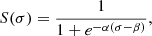 (11)
(11)
where α = 8.0 and β = 0.1 are empirical parameters controlling the sigmoid curve. The confidence weight is used to adjust the importance of the features; features with higher confidence receive greater weight, while features with lower confidence have less impact:
 (12)
(12)
 (13)
(13)
This method enables the model to adaptively process inputs of varying quality, effectively reducing the negative impact of low-confidence predictions. After processing through these two fusion units, features from different modalities are integrated, forming a joint representation vector F.
To enhance the model’s generalization ability in scenarios with scarce labeled data and incomplete features, we designed a semi-supervised learning loss function composed of multiple loss components, which jointly utilizes labeled and unlabeled hot subdwarf star samples for optimization:
 (14)
(14)
The supervised loss (Lsupervised) adopts an uncertainty-weighted cross-entropy formulation, in which the sample weights are dynamically adjusted according to the uncertainties predicted by the BNN. This allows the model to emphasize predictions with higher confidence. The unlabeled loss (Lunlabeled) leverages BNN predictions as soft labels for unlabeled data and minimizes the mean squared error between the fused model outputs and these soft labels, thereby exploiting a large pool of unlabeled candidates. To further enhance robustness, the consistency loss (Lconsistency) encourages the fused model outputs to remain consistent with BNN predictions in terms of single- and binary-star probabilities, facilitating cross-modal coordination. Finally, the embedding regularization term (Lembedding) constrains the fused representations to align with the classification logic embedded in the BNN latent space, ensuring structural consistency across modalities.
Based on extensive experimentation, the optimal weights were determined with α = 1.0, β = 0.3, γ = 0.1, and δ = 0.2. This strategy enables the model to effectively learn reliable classification representations, even under conditions of imbalanced samples and incomplete labels.
3.2.3. Training strategy
The model was trained using the AdamW optimizer with an initial learning rate of 1 × 10⁻⁴ and a weight decay of 1 × 10⁻⁵ (Loshchilov & Hutter 2019). To mitigate overfitting during the training process, we employed the ReduceLROnPlateau (Thakur et al. 2024) strategy. The learning rate was reduced by 50% if the validation loss did not improve for five consecutive epochs, and training was stopped if the validation loss did not improve for ten consecutive epochs to prevent overfitting. Data augmentation techniques, such as random masking and shifting, were applied to the spectral data to enhance the model’s robustness. During training, we used a mini-batch size of 32 for stochastic gradient descent. Experimental results show that the proposed cross-attention multimodal fusion model achieves significant advantages in the classification task of hot subdwarf binary systems, and the model’s classification results are analyzed in detail in Sect. 4.
4. Results
4.1. Evaluation criteria
To comprehensively evaluate the generalization ability of the proposed model in the binary classification task, various performance metrics were employed, including accuracy, precision, recall, F1 score, receiver operating characteristic (ROC) curve, and its area under the curve (AUC). These metrics enable evaluating the model’s classification performance from multiple dimensions. Accuracy represents the proportion of correctly predicted samples among all samples. Precision measures the proportion of actual hot subdwarf binary stars among those predicted as hot subdwarf binaries. Recall indicates the proportion of true hot subdwarf binaries correctly identified. F1-score is the harmonic mean of precision and recall, reflecting the balance between these two aspects of the model’s performance. The formulas for calculating these metrics are as follows:
 (15)
(15)
 (16)
(16)
 (17)
(17)
 (18)
(18)
where true positive (TP) represents the number of hot subdwarf binary stars correctly identified, true negative (TN) represents the number of samples correctly identified as non-binaries, while false positive (FP) and false negative (FN) refer to the number of samples incorrectly identified.
We also calculated the true negative rate (TNR) to assess the model’s ability to correctly identify single stars as well as the balanced accuracy, which is appropriate for imbalanced datasets. The positive predictive value (PPV) and negative predictive value (NPV) represent the proportion of correctly predicted binary and single star samples, respectively. Additionally, we computed the F1 scores for both binary stars (positive class) and single stars (negative class) to provide a comprehensive evaluation of the model’s performance on both categories.
4.2. Bayesian classification model results
Compared to the limited availability of spectroscopic observations, photometric data are far more abundant. Accordingly, a BNN model was first trained using photometric features. The dataset was split into training, validation, and test subsets in a ratio of 8:1:1, which were employed for model training, hyperparameter tuning, and performance evaluation, respectively.
One of the advantages of the BNN is its ability to quantify prediction uncertainty, which helps differentiate high-confidence predictions from ambiguous samples that require further validation. As shown in Fig. 3, the left panel illustrates the relationship between model prediction uncertainty and accuracy. As prediction uncertainty increases, the classification accuracy noticeably decreases, indicating that uncertainty estimation effectively reflects the reliability of the predictions. The right panel shows the relationship between prediction probability and uncertainty. The uncertainty follows a clear U-shaped trend: it is significantly higher when the prediction probability is near the decision boundary, around 0.5, and lower at the extremes of the probability scale, near 0 or 1.
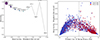 |
Fig. 3. Analysis of prediction uncertainties in the BNN model. Left: relationship between prediction uncertainty and classification accuracy, with point size indicating the number of samples at each uncertainty level. Right: relationship between the predicted probability of being a binary star and the corresponding uncertainty, where the red and blue points represent labeled binary and single star samples, respectively. |
The classification performance of the BNN model is summarized in Fig. 4. The confusion matrix shows that the model successfully identified most of the single and binary samples. As shown in Table 1, the model achieved an overall accuracy of 0.89, indicating good classification performance.
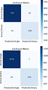 |
Fig. 4. Confusion matrices of the classification models. Top: confusion matrix of the BNN model on the test set. The vertical axis represents the true labels, and the horizontal axis represents the model’s predictions. Bottom: confusion matrix of the HsdB-FusionNet model on the sample set. In both panels, the numbers indicate the number of samples in each category, and the color intensity reflects the sample density. |
Comparison of classification performance metrics for different data types.
4.3. HsdB-FusionNet model results
HsdB-FusionNet takes a 128D spectral feature vector and a 32D photometric embedding vector as inputs to achieve more reliable classification results. Through cross-matching of the two modalities, we obtained 1,548 target objects, including 1281 single stars and 267 binary stars. Considering the limited sample size, we adopted a special data partitioning strategy: 100 samples (50 single stars and 50 binary stars) were randomly selected as a balanced test set, while the remaining 1448 samples were divided into training and validation sets in a 9:1 ratio. Additionally, to comprehensively evaluate the model’s performance, we also conducted an evaluation on the entire dataset.
From the confusion matrix, the classification performance of the model is clearly observed: out of 1274 samples that are true single stars, the model correctly predicted 1267 (TNs), with only seven incorrectly classified as binary stars (FPs); out of 267 true binary star samples, the model correctly predicted 238 (TPs), with 29 incorrectly classified as single stars (FNs). This indicates that the model achieves high precision in identifying single stars, and performs well in binary star recognition. Compared to the BNN classification model based on photometric data, this approach shows a significant improvement in binary star classification accuracy.
4.4. Feature attribution and model interpretability
To further understand the decision-making mechanisms of the BNN classification model based on photometric data and the HsdB-FusionNet model, which combines both spectroscopic and photometric data, we conducted a feature attribution analysis. This analysis includes the importance of photometric features as well as the attribution of spectroscopic features.
4.4.1. Feature importance analysis of the BNN classification model
To enhance the interpretability of the model, we used the SHapley Additive exPlanations (SHAP) method to evaluate the impact of each input feature on the predictions of the BNN (Ribeiro et al. 2016; Clare et al. 2022). Figure 5 shows the distribution of SHAP values, where the color scale ranges from blue (low feature values) to red (high feature values), and the horizontal axis represents the positive or negative contribution of each feature to the model’s output.
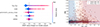 |
Fig. 5. Interpretability analysis of the BNN model. Left: feature importance evaluation using the SHAP method. The distribution of SHAP values for each feature is plotted, with the color scale from blue to red indicating feature values from low to high. Right: decision boundary of the BNN model in the GBP − GRP and RUWE 2D feature space. The background color represents the model’s predicted probability, with red corresponding to a binary classification and blue corresponding to a single star. The point colors denote the true sample labels. |
The analysis reveals that the color index GBP − GRP is the most influential feature in the model’s decision-making. Higher values of this feature are associated with higher predicted outputs, and are more likely to be classified as binary systems. This aligns with the prior knowledge that binary stars are typically redder in color. Next, RUWE also has a significant impact. Larger RUWE values indicate a poorer fit to the Gaia single-source astrometric solution and may reflect unresolved orbital or photocenter motion in binary systems. This is consistent with the expectation that some unresolved binaries can show enhanced astrometric residuals. Additionally, astrometric excess noise, Plx, and GMAG also slightly affect the model.
Figure 5 plots the 2D decision boundary of the BNN model. It can be observed that the model predominantly classifies samples with redder colors and larger astrometric residuals into the binary star region (upper-right red zone), while bluer samples with lower astrometric residuals tend to cluster in the single-star region (lower-left blue zone). This result is consistent with the findings from the SHAP analysis.
4.4.2. Interpretability analysis of the HsdB-FusionNet model
To verify whether the decision-making mechanism of the fusion model in the hot subdwarf single and binary classification task is consistent with prior knowledge, we conducted attribution analysis on the 128D spectral feature vectors using the integrated gradients (IG) method (Sundararajan et al. 2017; Wang et al. 2024). Integrated gradients quantifies the marginal contribution of each feature to the model output by accumulating gradients along the path between the input features and a reference baseline. To map the 128D IG attribution values back to the original wavelength space, we adopted a Jacobian projection approach (Ipbüker & Bildirici 2002; Birgin et al. 2014). Specifically, this involves computing the gradient of each feature unit with respect to the original spectral pixels, combining it with the receptive field of each feature, distributing the attribution values to wavelength pixels according to the gradient weights, and accumulating them over the full spectrum to obtain an attribution curve one-to-one aligned with the physical wavelength. We separately computed attribution values for single-class and binary-class samples in the test set, obtaining the binary-class IG, single-class IG, and their difference (ΔIG) distributions in the spectral space.
The results (Fig. 6) show that significant attribution peaks are concentrated in the 3800–4900 Å range, corresponding to higher-order Balmer lines (e.g., Hδ 4102 Å, Hγ 4341 Å, and Hβ 4861 Å) and certain He I/He II absorption lines (e.g., He I 4026 Å, He II 4686 Å). The core of the model’s decision-making lies in exploiting the modulation of Balmer and He absorption line morphology by companion-star light dilution. These lines exhibit notable morphological differences between single and binary hot subdwarf systems. In binary systems, the continuum emission from the companion star, often an F-, G-, or K-type MS star, dilutes the Balmer and helium absorption lines of the hot subdwarf, making them shallower and broader. In single systems, these absorption lines retain greater depth and sharpness. In the binary-class IG, the above wavelength ranges display strong positive attributions, indicating that the model regards these dilution features as binary indicators. In the single-class IG, the same ranges are predominantly negative, corresponding to strong absorption signals used to identify single stars. The ΔIG distribution further confirms that positive peaks correspond to companion-induced dilution effects in binaries, while negative peaks correspond to strong absorption features in singles.
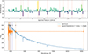 |
Fig. 6. IG attribution and its mapping to original wavelength space for HsdB-FusionNet model. (Top) IG attribution distribution for the 128D spectral feature vector, where colors indicate the signed importance (positive values denote features favoring binary classification, while negative values denote features favoring single classification). (Bottom) Mapping of the signed attribution values to the original spectral wavelength space using the Jacobian projection method. The blue curve represents the observed spectral flux, and the orange curve shows the wavelength-resolved signed attribution values, where positive peaks (orange shadow) correspond to wavelength regions important for identifying binaries. The negative peaks (purple shadow) correspond to regions important for identifying singles. The vertical shaded areas indicate wavelength ranges with the highest absolute attribution values. |
4.5. Comparison of different data types
In the following, we compare the performance of three models in our experiments. The first used photometric and astrometric features and was classified with BNN. The second relied on spectral data, where a feature extraction model generated 128D features that were then classified with a multilayer perceptron. The third employed multimodal fusion of photometric and spectral data through cross-attention mechanisms followed by multilayer perceptron classification. The classification performance results are shown in Table 1.
The results clearly demonstrate that the fusion model significantly outperforms models that use only photometric or spectral data across all metrics. Specifically, the fusion model achieves an accuracy of 0.9767, compared to 0.8954 for the photometric-only model and 0.9313 for the spectral-only model, indicating a substantial improvement in classification performance. This indicates that multimodal data fusion effectively leverages the complementary information from both data types, greatly enhancing the model’s discriminative ability.
5. Applications
To validate the model’s generalization capability and provide more samples for subsequent scientific research, we applied the developed multimodal fusion model to the hot subdwarf candidate catalog proposed by Culpan et al. (2022). The catalog contains 61 585 hot subdwarf candidates.
5.1. Extended to larger catalogs
We first cross-matched these candidates with SDSS DR18 and successfully obtained spectral data for 3230 candidates. We further cross-matched these 3230 objects with Gaia DR3 to acquire key astrometric parameters. We first applied the trained BNN classification model to perform an initial classification of the 3230 objects based on five photometric and astrometric features. Subsequently, we extracted the corresponding 32D photometric embedding vectors for each object from the BNN model. Meanwhile, we utilized the trained spectral feature extraction model to extract features from the spectroscopic data of these objects, generating 128D spectral feature vectors. Finally, we combined photometric embedding vectors, spectral feature vectors, and BNN prediction probabilities along with their uncertainties as inputs to the trained multimodal fusion model for the final binary identification.
5.2. Classification results and analysis of candidates
Through the above process, we obtained detailed classification results. Using the BNN classification model with only photometric features, we identified 1838 single star candidates and 1392 binary star candidates. After further classification with the fusion model, 1861 single star candidates and 1369 binary star candidates were determined.
This corresponds to an apparent binary-candidate fraction of approximately 40% within the SDSS-matched candidate subsample. This value is higher than the ∼17–20% fractions reported in recent SED- or Gaia-XP-based studies of composite hot subdwarf systems (Vázquez et al. 2024; Ambrosch et al. 2026). This difference is likely related to both sample selection and methodology. In particular, SED-based searches are mainly sensitive to systems with luminous cool companions that produce detectable IR excess, whereas our multimodal model combines Gaia photometric and astrometric diagnostics with SDSS spectroscopic information. Therefore, it may recover additional binary candidates whose signatures are reflected in astrometric residuals or spectroscopic features rather than in strong SED excess alone. We emphasize that this value represents an apparent fraction in the SDSS-matched candidate subsample, rather than the intrinsic binary fraction of the full hot subdwarf population.
5.2.1. Color-magnitude diagram of candidates
To visually validate the classification model, we constructed a color-magnitude diagram of the candidates based on Gaia data and labeled the single and binary star candidates separately. As shown in Fig. 7, the model-predicted single star objects are primarily concentrated in the typical hot subdwarf region, while the binary star candidates extend noticeably toward the red end and lower luminosity, exhibiting greater dispersion. This distribution trend aligns with the flux contribution of companion star spectra, especially in the IR, leading to the observations of redder color and decreased brightness. Overall, these results support the reliability of the fusion model in binary star identification and provide a reference for subsequent sample selection and target prioritization.
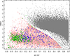 |
Fig. 7. Color-magnitude diagram of candidates. The blue points represent the binary star candidates predicted by the model; the green points represent the single star candidates; the pink points show the overall distribution of hot subdwarf candidates; and the gray points represent reference background stars. |
5.2.2. Infrared excess and SED fitting validation
Composite systems consisting of hot subdwarfs and cool MS stars often exhibit IR excess in the near-IR band. Thejll et al. (1995) and Ulla & Thejll (1998) noted that this phenomenon is primarily caused by the radiation from A–K type companion stars. Solano et al. (2022) proposed a method for identifying binary systems using SED fitting through the VOSA tool, assessing whether the flux in the IR band significantly exceeds that of the single star model. Based on an analysis of 2MASS data, Stark & Wade (2003) found that approximately 30%−40% of sdB or sdO stars exhibit IR excess in the J–Ks color, indicating that they are composite systems. Schaffenroth et al. (2022) further combined TESS and K2 light curves with Gaia data to identify over a hundred binary systems with M-type or BD companions. Through SED fitting, they confirmed that the IR excess originates from irradiation heating of the companion, which produces a reflection effect.
Based on the above, we used the Virtual Observatory Tool (VOSA; Bayo et al. 2008) to construct SEDs of these candidates from the ultraviolet to IR bands. We then performed fitting analysis to search for significant IR excess and further assess the reliability of the binary-star candidates identified by the model.
VOSA is a tool developed by the Spanish Virtual Observatory that compares catalog photometry with different collections of theoretical models and determines which model best reproduces the observed data following different statistical approaches, and then estimates the atmospheric parameters of each object from the best-fitting model. In our analysis, the photometric information was derived from the following catalogs: Gaia EDR3 (Gaia Collaboration 2016), 2MASS (Skrutskie et al. 2006), WISE (Wright et al. 2010), Pan-STARRS1 (Chambers et al. 2016), and SDSS DR11 /DR12 (Alam et al. 2015).
The fitting algorithm used by VOSA is an extension of the method developed by Lada et al. (2006). The basic idea is to begin at wavelengths λ ≥ 21500 Å, and perform a linear regression fit in the log νFν versus log ν space of the observed SED to preliminarily assess whether there is an upward trend in the IR. Subsequently, VOSA sequentially adds new photometric points in the IR bands and recalculates the slope changes, gradually confirming whether there is a systematic deviation in IR flux. This iterative process makes the identification of IR excess more robust, allowing for the elimination of FPs caused by individual data point errors.
After completing the SED fitting, VOSA compares the observed flux with the synthesized flux from the best-fit model at each point and quantitatively assesses the statistical deviation. If the observed flux in a given band is significantly higher than the model’s prediction, it is classified as IR excess. Additionally, VOSA can provide uncertainty estimates for each parameter based on fitting residuals, which serves as a basis for further analysis. Based on the fitting results, we categorized all 1369 binary star candidates into four groups based on the completeness of the IR photometric data and the significance of excess, as shown in Table 2.
Classification by mid-IR photometry completeness and excess significance
The results show that objects with clear IR excess features account for only 6% of the total sample. However, considering the limited observational depth of the W3/W4 bands and that IR data for most targets are still at the upper limit, this percentage is likely underestimated. Among them, objects in the det category (53%) have good W1/W2 observed data, showing potential for detecting IR excess, making them the preferred targets for subsequent mid-IR observations. Objects in the partial category (33%) have coverage beyond 5 μm, but lack actual measurements and only have upper limits, often exhibiting a tail-up feature in the SED, indicating suspicious characteristics. The censored category (9%) lacks key mid-IR information, representing left-censored samples, which are not verifiable and thus excluded from further analysis.
Furthermore, we selected 82 objects from the excess category for binary fit analysis. The results show that for most objects, the fit residuals (Vgfb) under the binary fit are significantly high, with large fitting uncertainties, and the companion star temperatures tend to be overestimated (averaging above 10 000 K). This phenomenon may stem from the low signal-to-noise ratio (S/N) of UV band observations or insufficient handling of UV absorption in the model, leading to a bias in the fitting of the thermal source.
Therefore, we set a fitting quality threshold and only selected objects with Vgfb < 5 as reliable binary fit subsamples for subsequent parameter analysis and statistical distribution studies, including key physical indicators such as companion star temperature, flux contribution, and the relationship between the primary and companion star temperatures.
5.2.3. Binary parameters and system properties analysis
Due to the limited availability of mid-IR measurements for the det and partial categories, we conducted a detailed analysis of 1176 candidates from these two groups to evaluate their likelihood of being binary systems. We first performed single fit and binary fit SED chi-square fitting for each candidate. We assessed how well the binary model improved the fit by comparing its chi-square values with those of the single fit. Specifically, the improvement in model fitting is defined as
 (19)
(19)
When χratio ≥ 1.2, it is considered that the binary model significantly improves the statistical fit compared to the single-star model, further supporting the possibility that the target is a genuine binary system. The fitting results show that 92% of the objects (1081/1176) exhibit better χ2 values under the binary fit, and 86.1% of the objects (1013/1176) show a χ2 improvement greater than 20%. Among these targets, 904 objects have a Vgfb ≤15 under the binary fit, indicating that most of the targets have a good fitting quality. These results clearly demonstrate that, even in the absence of sufficient measured data in the long-wavelength bands, the binary model significantly improves the SED fitting, supporting the possibility of these candidates being true binary systems.
Additionally, we performed binary model fitting on the excess category, which has clear IR excess markers. It was found that although some candidates in this category had poor fitting quality (higher Vgfb values and abnormally high companion star temperatures), 14 candidates exhibited good fitting quality (Vgfb < 5). Combining the 565 candidates from the det and partial categories, which showed significant improvement in fitting (χratio2 ≥ 1.2) and good fitting quality (Vgfb < 5), we ultimately selected a total of 579 candidates with good fitting quality for subsequent statistical analysis of companion star parameters.
To visually present the fitting features of these 579 candidates and the distribution of companion star parameters, we further plotted typical SED fitting examples, as shown in Fig. 8, while the statistical distribution of the companion star parameters is presented through a multidimensional statistical chart, as shown in Fig. 9. The effective temperatures of the companion stars are mostly concentrated in the range of 5000–10 000 K, which is consistent with previous studies, indicating that these companion stars are primarily late-type MS stars or subgiants. Additionally, the companion stars contribute a significant proportion to the overall SED flux of the system, with typical values around 80%–90%, confirming the dominant role of the companion stars in the SEDs of these systems. At the same time, most of the selected samples have low Vgfb values, indicating that the fitting results are reliable and trustworthy.
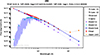 |
Fig. 8. SED fitting example for binary star candidate. The red circles represent the observed photometry; and the blue solid line represents the best-fit binary combination model with the primary star shown as a purple line and the companion star as a light blue line. The orange inverted triangles indicate the upper limits for unmeasured photometric points. |
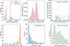 |
Fig. 9. Statistical analysis of the companion star parameters for our binary star candidates. Top left: distribution of the effective temperatures for the primary and companion stars. Top middle: probability density distribution of the companion star effective temperatures. Top right: correlation between the primary and companion star temperatures. Bottom left: distribution of the companion star flux contribution ratios. Bottom middle: distribution of the chi-square ratio values for the single-star vs. binary model fits. Bottom right: distribution of the Vgfb fitting quality. |
5.3. Candidate catalog
We constructed a catalog of hot subdwarf binary star candidates, whose complete version is available through online resources. This catalog summarizes the binary star candidates selected through a two-stage classification strategy. Additionally, we utilized the VOSA tool to perform confirmation on some of the candidates and provided corresponding parameter estimates.
The catalog contains a total of 1369 binary star candidates, with 1258 of them having observable data available for VOSA fitting. Among them, 111 samples lack measured data in the WISE IR bands (W1–W4), making reliable SED fitting impossible. Another 82 samples were flagged as IR excess and exhibited large fitting residuals (Vgfb > 15). Only 44 samples from the excess group yielded good fitting results (Vgfb < 15). For the remaining 1176 samples with partial data missing but not flagged as IR excess, we performed a comparison between single fit and binary fit. We found that approximately 86% (1013 samples) showed a reduction in fitting residuals greater than 20% when the binary model was applied, indicating that the binary model is more plausible for these samples. We further selected subsamples with Vgfb < 5 and obtained detailed physical parameter estimates for both the primary and companion stars in 579 binary systems.
6. Summary and conclusions
We developed a novel multimodal deep learning framework, HsdB-FusionNet, which integrates photometric and spectroscopic data to significantly enhance the accuracy and stability of hot subdwarf binary identification. Compared to traditional single-modality methods, our fusion model effectively captures complementary observational features, achieving a high precision of 97.1% in binary classifications. Furthermore, through SHAP values and IG analysis, we confirmed that the model’s decision making is broadly consistent with prior astrophysical knowledge. Specifically, the model correctly anchors on physically meaningful Gaia features, including the photometric color index GBP − GRP and astrometric diagnostics such as RUWE, as well as critical spectral regions including the Balmer, He II, and nebular emission lines.
In practical applications, we applied HsdB-FusionNet to a massive catalog of 61 585 hot subdwarf candidates. This resulted in the successful identification of 1369 binary candidates. Subsequent SED fitting robustly validated the binary nature of these candidates (with 1176 systems undergoing detailed fitting comparisons). Most importantly, we successfully extracted the atmospheric parameters for both primary and companion stars in a high-quality subset of 579 binary systems.
To accommodate the feature missingness in real astronomical data, we also proposed a missing data handling strategy based on a masking mechanism, avoiding the wastage of hot subdwarf binary samples by directly deleting incomplete samples. This ensures the robustness and generalizability of the model under conditions of incomplete observational information. At the same time, the candidate catalog we constructed provides rich supplementary information, including the classification probabilities output by the model, and the atmospheric parameters estimated by VOSA. These efforts not only provide advanced tools for efficiently handling large-scale data but also significantly expand the existing population of hot subdwarf binary stars.
In the future, we plan to extend this method to the joint analysis of light curves, multi-epoch spectral, and Gaia astrometric data. In addition, we aim to extend binary classification to encompass a wider range of systems, including eclipsing binaries, HW Vir systems, and reflection-effect systems. Given its strong capability in multimodal data processing, our model can be broadly applied to next-generation survey missions such as CSST, LSST, and DESI, thereby advancing the study of extreme stellar systems and binary evolution in the Milky Way.
Data availability
The catalogue is available at the CDS via https://cdsarc.cds.unistra.fr/viz-bin/cat/J/A+A/711/A217
Acknowledgments
This study was supported by the Natural Science Foundation of Shandong Province under grant Nos. ZR2024MA063, ZR2022MA076, and ZR2022MA089, ZR2025MS06. Additional funding was provided by the science research grants of the China Manned Space Project under Grant Nos. CMS-CSST-2021-B05 and CMS-CSST-2021-A08. The research was also supported by the National Natural Science Foundation of China (NSFC) under grant Nos. 12573109, 11873037 and 11803016. Furthermore, the Young Scholars Program of Shandong University, Weihai (2016WHWLJH09) provided support for this research.
References
- Alam, S., Albareti, F. D., Allende Prieto, C., et al. 2015, ApJS, 219, 12 [Google Scholar]
- Ambrosch, M., Viscasillas Vázquez, C., Solano, E., et al. 2026, A&A, 708, A23 [NASA ADS] [CrossRef] [EDP Sciences] [Google Scholar]
- Babusiaux, C., Van Leeuwen, F., Barstow, M. A., et al. 2018, A&A, 616, A10 [NASA ADS] [CrossRef] [EDP Sciences] [Google Scholar]
- Bayo, A., Rodrigo, C., Navascués, D. B., et al. 2008, A&A, 492, 277 [NASA ADS] [CrossRef] [EDP Sciences] [Google Scholar]
- Birgin, E. G., Martínez, J. M., & Raydan, M. 2014, J. Stat. Softw., 60, 1 [CrossRef] [Google Scholar]
- Bu, Y., Lei, Z., Zhao, G., Bu, J., & Pan, J. 2017, ApJS, 233, 2 [NASA ADS] [CrossRef] [Google Scholar]
- Bu, Y., Zeng, J., Lei, Z., & Yi, Z. 2019, ApJ, 886, 128 [NASA ADS] [CrossRef] [Google Scholar]
- Chambers, K. C., Magnier, E. A., Metcalfe, N., et al. 2016, ArXiv e-prints [arXiv:1612.05560] [Google Scholar]
- Charpinet, S., Fontaine, G., Brassard, P., Green, E., & Chayer, P. 2005, A&A, 437, 575 [NASA ADS] [CrossRef] [EDP Sciences] [Google Scholar]
- Cheng, Z., Kong, X., Wu, T., et al. 2024, ApJS, 274, 2 [Google Scholar]
- Clare, M. C., Sonnewald, M., Lguensat, R., Deshayes, J., & Balaji, V. 2022, JAMES, 14, e2022MS003162 [Google Scholar]
- Cui, Z., Chen, W., & Chen, Y. 2016, [arXiv:1603.06995] [Google Scholar]
- Culpan, R., Geier, S., Reindl, N., et al. 2022, A&A, 662, A40 [NASA ADS] [CrossRef] [EDP Sciences] [Google Scholar]
- Drilling, J., Jeffery, C., Heber, U., Moehler, S., & Napiwotzki, R. 2013, A&A, 551, A31 [NASA ADS] [CrossRef] [EDP Sciences] [Google Scholar]
- Fontaine, G., Brassard, P., Charpinet, S., et al. 2003, ApJ, 597, 518 [Google Scholar]
- Gaia Collaboration (Prusti, T., et al.) 2016, A&A, 595, A1 [NASA ADS] [CrossRef] [EDP Sciences] [Google Scholar]
- Geier, S., Hirsch, H., Tillich, A., et al. 2011, A&A, 530, A28 [NASA ADS] [CrossRef] [EDP Sciences] [Google Scholar]
- Geier, S., Østensen, R. H., Nemeth, P., et al. 2017, A&A, 600, A50 [NASA ADS] [CrossRef] [EDP Sciences] [Google Scholar]
- Graves, A. 2011, NeurIPS, 24 [Google Scholar]
- Guo, Y., Liu, Z., Krishnswamy, P., & Ramasamy, S. 2019, ArXiv e-prints [arXiv:1911.07572] [Google Scholar]
- Han, Z., Podsiadlowski, P., Maxted, P. F., Marsh, T. R., & Ivanova, N. 2002, MNRAS, 336, 449 [NASA ADS] [CrossRef] [Google Scholar]
- Han, Z.-W., Podsiadlowski, P., Maxted, P. F., & Marsh, T. R. 2003, MNRAS, 341, 669 [NASA ADS] [CrossRef] [Google Scholar]
- Han, Z., Podsiadlowski, P., & Lynas-Gray, A. 2010, Ap&SS, 329, 41 [NASA ADS] [CrossRef] [Google Scholar]
- Heber, U. 2009, ARA&A, 47, 211 [Google Scholar]
- Heber, U. 2016, PASP, 128, 082001 [Google Scholar]
- Humason, M., & Zwicky, F. 1947, ApJ, 105, 85 [NASA ADS] [CrossRef] [Google Scholar]
- Iben, I., Jr, & Tutukov, A. V. 1986, ApJ, 311, 742 [NASA ADS] [CrossRef] [Google Scholar]
- Ipbüker, C., & Bildirici, I. Ö. 2002, in Proceedings of the Third International Symposium Mathematical & Computational Applications, 175 [Google Scholar]
- Jospin, L. V., Laga, H., Boussaid, F., Buntine, W., & Bennamoun, M. 2022, IEEE Comput. Intell. Mag., 17, 29 [Google Scholar]
- Kilkenny, D., Koen, C., O’donoghue, D., & Stobie, R. 1997, MNRAS, 285, 640 [NASA ADS] [CrossRef] [Google Scholar]
- Kilkenny, D., Heber, U., & Drilling, J. 1988, SAAOC, 80, 12 [Google Scholar]
- Kononenko, I. 1989, Biol. Cybern., 61, 361 [Google Scholar]
- Kupfer, T., Geier, S., Heber, U., et al. 2015, A&A, 576, A44 [NASA ADS] [CrossRef] [EDP Sciences] [Google Scholar]
- Kupfer, T., Bauer, E. B., Burdge, K. B., et al. 2020, ApJ, 898, L25 [Google Scholar]
- Lada, C. J., Muench, A. A., Luhman, K., et al. 2006, AJ, 131, 1574 [Google Scholar]
- Lei, Z., Zhao, J., Németh, P., & Zhao, G. 2018, ApJ, 868, 70 [Google Scholar]
- Lei, Z., Zhao, J., Németh, P., & Zhao, G. 2019, ApJ, 881, 135 [NASA ADS] [CrossRef] [Google Scholar]
- Lei, Z., Zhao, J., Németh, P., & Zhao, G. 2020, ApJ, 889, 117 [NASA ADS] [CrossRef] [Google Scholar]
- Lei, Z., He, R., Nemeth, P., et al. 2023, ApJ, 942, 109 [CrossRef] [Google Scholar]
- Lisker, T., Heber, U., Napiwotzki, R., et al. 2005, A&A, 430, 223 [NASA ADS] [CrossRef] [EDP Sciences] [Google Scholar]
- Liu, W., Bu, Y., Kong, X., Yi, Z., & Liu, M. 2024, PASJ, 76, 329 [Google Scholar]
- Loshchilov, I., & Hutter, F. 2019, in International Conference on Learning Representations [Google Scholar]
- Luo, Y., Nemeth, P., Deng, L., & Han, Z. 2019, ApJ, 881, 7 [NASA ADS] [CrossRef] [Google Scholar]
- Luo, Y., Nemeth, P., Wang, K., Wang, X., & Han, Z. 2021, ApJS, 256, 28 [NASA ADS] [CrossRef] [Google Scholar]
- Maxted, P., Heber, U., Marsh, T., & North, R. 2001, MNRAS, 326, 1391 [CrossRef] [Google Scholar]
- Molina, F., Vos, J., Németh, P., et al. 2022, A&A, 658, A122 [NASA ADS] [CrossRef] [EDP Sciences] [Google Scholar]
- Mullachery, V., Khera, A., & Husain, A. 2018, ArXiv e-prints [arXiv:1801.07710] [Google Scholar]
- Nah, S., Hyun Kim, T., & Mu Lee, K. 2017, in Proceedings of the IEEE Conference on Computer Vision and Pattern Recognition, 3883 [Google Scholar]
- Németh, P., Vos, J., Molina, F., & Bastian, A. 2021, A&A, 653, A3 [Google Scholar]
- O’Connell, R. W. 1999, ARA&A, 37, 603 [CrossRef] [Google Scholar]
- Østensen, R. H., Silvotti, R., Charpinet, S., et al. 2010, MNRAS, 409, 1470 [CrossRef] [Google Scholar]
- Ostrowski, J., Baran, A. S., Sanjayan, S., & Sahoo, S. 2021, MNRAS, 503, 4646 [NASA ADS] [CrossRef] [Google Scholar]
- Pelisoli, I., Vos, J., Geier, S., Schaffenroth, V., & Baran, A. S. 2020, A&A, 642, A180 [NASA ADS] [CrossRef] [EDP Sciences] [Google Scholar]
- Peng, K. C., & Chen, T. 2015, in 2015 IEEE International Conference on Multimedia and Expo, 1 [Google Scholar]
- Ranaivomanana, P., Uzundag, M., Johnston, C., et al. 2025, A&A, 693, A268 [NASA ADS] [CrossRef] [EDP Sciences] [Google Scholar]
- Reed, M., Kawaler, S. D., Østensen, R. H., et al. 2010, MNRAS, 409, 1496 [NASA ADS] [CrossRef] [Google Scholar]
- Ribeiro, M. T., Singh, S., & Guestrin, C. 2016, in Proceedings of the 22nd ACM SIGKDD Conference on Knowledge Discovery and Data Mining, 1135 [Google Scholar]
- Rodrigo, C., & Solano, E. 2020, in XIV. 0 Scientific Meeting (virtual) of the Spanish Astronomical Society, 182 [Google Scholar]
- Schaffenroth, V., Pelisoli, I., Barlow, B. N., Geier, S., & Kupfer, T. 2022, A&A, 666, A182 [NASA ADS] [CrossRef] [EDP Sciences] [Google Scholar]
- Schaffenroth, V., Barlow, B., Pelisoli, I., Geier, S., & Kupfer, T. 2023, A&A, 673, A90 [NASA ADS] [CrossRef] [EDP Sciences] [Google Scholar]
- Seo, M., Kembhavi, A., Farhadi, A., & Hajishirzi, H. 2017, in International Conference on Learning Representations [Google Scholar]
- Skrutskie, M. F., Cutri, R. M., Stiening, R., et al. 2006, AJ, 131, 1163 [NASA ADS] [CrossRef] [Google Scholar]
- Solano, E., Ulla, A., Pérez-Fernández, E., et al. 2022, MNRAS, 514, 4239 [NASA ADS] [CrossRef] [Google Scholar]
- Soydaner, D. 2022, Neural Comput. Appl., 34, 13371 [Google Scholar]
- Stark, M. A., & Wade, R. A. 2003, AJ, 126, 1455 [NASA ADS] [CrossRef] [Google Scholar]
- Sun, S., Zhang, G., Shi, J., & Grosse, R. 2019, in International Conference on Learning Representations [Google Scholar]
- Sundararajan, M., Taly, A., & Yan, Q. 2017, in International Conference on Machine Learning, PMLR, 3319 [Google Scholar]
- Taam, R. E., & Sandquist, E. L. 2000, ARA&A, 38, 113 [NASA ADS] [CrossRef] [Google Scholar]
- Tan, L., Mei, Y., Liu, Z., et al. 2022, ApJS, 259, 5 [NASA ADS] [CrossRef] [Google Scholar]
- Thakur, A., Gupta, M., Sinha, D. K., et al. 2024, Int. J. Comput. Intell. Syst., 17, 1 [Google Scholar]
- Thejll, P., Ulla, A., & MacDonald, J. 1995, A&A, 303, 773 [Google Scholar]
- Ulla, A., & Thejll, P. 1998, A&AS, 132, 1 [NASA ADS] [CrossRef] [EDP Sciences] [Google Scholar]
- Uzundag, M., Krzesinski, J., Pelisoli, I., et al. 2024, A&A, 684, A118 [NASA ADS] [CrossRef] [EDP Sciences] [Google Scholar]
- Vasishta, S. 2025, Stellar Structure and Evolution: A Comprehensive Guide (Delhi: Educohack Press) [Google Scholar]
- Vázquez, C. V., Solano, E., Ulla, A., et al. 2024, A&A, 691, A223 [NASA ADS] [CrossRef] [EDP Sciences] [Google Scholar]
- Vos, J., Németh, P., Vučković, M., Østensen, R., & Parsons, S. 2018, MNRAS, 473, 693 [NASA ADS] [CrossRef] [Google Scholar]
- Wang, Y., Zhang, T., Guo, X., & Shen, Z. 2024, ArXiv e-prints [arXiv:2403.10415] [Google Scholar]
- Wen, Y., Vicol, P., Ba, J., Tran, D., & Grosse, R. 2018, in International Conference on Learning Representations [Google Scholar]
- Wright, E. L., Eisenhardt, P. R. M., Mainzer, A. K., et al. 2010, AJ, 140, 1868 [Google Scholar]
- Wu, H., Bu, Y., Zhang, J., et al. 2025, A&A, 693, A245 [NASA ADS] [CrossRef] [EDP Sciences] [Google Scholar]
- Xiong, H., Chen, X., Podsiadlowski, P., Li, Y., & Han, Z. 2017, A&A, 599, A54 [NASA ADS] [CrossRef] [EDP Sciences] [Google Scholar]
- Yang, B., Bu, Y., Zhang, Y., et al. 2026, A&A, 710, A319 [NASA ADS] [CrossRef] [EDP Sciences] [Google Scholar]
- Zhang, X., & Jeffery, C. S. 2012, MNRAS, 419, 452 [NASA ADS] [CrossRef] [Google Scholar]
- Zhang, J., Bu, Y., Wu, H., et al. 2025, AJ, 170, 94 [Google Scholar]
Appendix A: Validation of feature extraction modules
To validate the effectiveness of the feature extraction modules, we first conducted a visual analysis of the 32D photometric embeddings derived from the BNN. Specifically, we selected the two most informative dimensions and constructed a 2D embedding space to visualize the distribution of samples. Figure A.1 shows a clear structural separation between single and binary systems: binary stars tend to cluster in regions of high predicted probability, whereas single stars predominantly lie in low-probability regions. This indicates that the intermediate representations learned by the BNN possess strong discriminative power for the binary classification task. The embedding space successfully captures the underlying structural differences between the two classes, providing a solid foundation for subsequent spectral feature fusion.
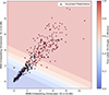 |
Fig. A.1. 2D visualization of the embedding feature space extracted from the BNN. The x- and y-axes correspond to the two most informative latent dimensions. The blue and red points represent single and binary hot subdwarf stars, respectively. The background color map indicates the model’s predicted probability, ranging from blue (low binary probability) to red (high binary probability), illustrating the decision boundary structure. |
On the other hand, to assess the representational capacity of the spectral feature extraction module, we evaluated its performance in reconstructing the original stellar spectra. As shown in Fig. A.2, the reconstructed spectra closely match the observed spectra across the entire wavelength range (3800–9000 Å). In particular, both the continuum shape and major absorption lines are accurately reproduced. The zoomed-in view further demonstrates the model’s ability to recover critical spectral line features, such as hydrogen and helium absorption lines. Although minor smoothing is observed in line depths, essential attributes including line positions, widths, and intensities are well preserved. Residual analysis indicates that reconstruction errors are primarily concentrated around strong absorption lines, while residuals across other regions remain small and stable. These results confirm that the learned 128D spectral embeddings effectively capture the spectral characteristics of hot subdwarf stars.
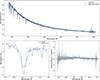 |
Fig. A.2. Analysis of the reconstruction performance of the spectral feature extraction network. (Top) Comparison between the original and reconstructed full-spectrum profiles. (Bottom left) Zoom-in on regions with prominent spectral line reconstruction errors. (Bottom right) residual distribution between the reconstructed and observed spectra. |
All Tables
All Figures
|
Fig. 1. Architecture of the BNN. The model consists of three main components. (1) Input processing layer: The input feature matrix X, possibly containing missing values, is accompanied by a binary mask indicating valid entries (features ≠ −999), followed by standardization. (2) Masked hidden layer: The standardized features are combined with the mask via the Hadamard product to obtain masked features, which are processed through two hidden layers with Bayesian weight distributions and dropout regularization. (3) Prediction layer: The output layer produces a Bayesian predictive distribution, evaluated through five-fold cross-validation. Model performance was assessed using accuracy, confusion matrices, and uncertainty quantification. |
| In the text | |
|
Fig. 2. Architecture of the HsdB-FusionNet. (a) Top: simplified pipeline of the SFE. The spectrum (∼3800 dims) is processed by multi-scale 1D convolutions (kernels k = {3, 9, 27}) and residual blocks to capture local and cross-scale patterns. Their features are fused through a main path and a line path, and the decoder predicts the reconstructed spectrum together with its continuum and line components. (b) Bottom: overall architecture of HsdB-FusionNet. The network consumes three inputs – SFE spectral features S, BNN embeddings B, and BNN auxiliary uncertainty (σ, p), which pass through spectral-wise and BNN-wise attention streams and fully connected layers. The fusion module combines a cross-attention unit (S → B, B → S) with an uncertainty-weighted unit using Sigmoid scaling (gated by σ). The concatenated representation is fed to multilayer perceptron (MLP) heads and a classifier to output the hot-subdwarf single and binary probability. |
| In the text | |
|
Fig. 3. Analysis of prediction uncertainties in the BNN model. Left: relationship between prediction uncertainty and classification accuracy, with point size indicating the number of samples at each uncertainty level. Right: relationship between the predicted probability of being a binary star and the corresponding uncertainty, where the red and blue points represent labeled binary and single star samples, respectively. |
| In the text | |
|
Fig. 4. Confusion matrices of the classification models. Top: confusion matrix of the BNN model on the test set. The vertical axis represents the true labels, and the horizontal axis represents the model’s predictions. Bottom: confusion matrix of the HsdB-FusionNet model on the sample set. In both panels, the numbers indicate the number of samples in each category, and the color intensity reflects the sample density. |
| In the text | |
|
Fig. 5. Interpretability analysis of the BNN model. Left: feature importance evaluation using the SHAP method. The distribution of SHAP values for each feature is plotted, with the color scale from blue to red indicating feature values from low to high. Right: decision boundary of the BNN model in the GBP − GRP and RUWE 2D feature space. The background color represents the model’s predicted probability, with red corresponding to a binary classification and blue corresponding to a single star. The point colors denote the true sample labels. |
| In the text | |
|
Fig. 6. IG attribution and its mapping to original wavelength space for HsdB-FusionNet model. (Top) IG attribution distribution for the 128D spectral feature vector, where colors indicate the signed importance (positive values denote features favoring binary classification, while negative values denote features favoring single classification). (Bottom) Mapping of the signed attribution values to the original spectral wavelength space using the Jacobian projection method. The blue curve represents the observed spectral flux, and the orange curve shows the wavelength-resolved signed attribution values, where positive peaks (orange shadow) correspond to wavelength regions important for identifying binaries. The negative peaks (purple shadow) correspond to regions important for identifying singles. The vertical shaded areas indicate wavelength ranges with the highest absolute attribution values. |
| In the text | |
|
Fig. 7. Color-magnitude diagram of candidates. The blue points represent the binary star candidates predicted by the model; the green points represent the single star candidates; the pink points show the overall distribution of hot subdwarf candidates; and the gray points represent reference background stars. |
| In the text | |
|
Fig. 8. SED fitting example for binary star candidate. The red circles represent the observed photometry; and the blue solid line represents the best-fit binary combination model with the primary star shown as a purple line and the companion star as a light blue line. The orange inverted triangles indicate the upper limits for unmeasured photometric points. |
| In the text | |
|
Fig. 9. Statistical analysis of the companion star parameters for our binary star candidates. Top left: distribution of the effective temperatures for the primary and companion stars. Top middle: probability density distribution of the companion star effective temperatures. Top right: correlation between the primary and companion star temperatures. Bottom left: distribution of the companion star flux contribution ratios. Bottom middle: distribution of the chi-square ratio values for the single-star vs. binary model fits. Bottom right: distribution of the Vgfb fitting quality. |
| In the text | |
|
Fig. A.1. 2D visualization of the embedding feature space extracted from the BNN. The x- and y-axes correspond to the two most informative latent dimensions. The blue and red points represent single and binary hot subdwarf stars, respectively. The background color map indicates the model’s predicted probability, ranging from blue (low binary probability) to red (high binary probability), illustrating the decision boundary structure. |
| In the text | |
|
Fig. A.2. Analysis of the reconstruction performance of the spectral feature extraction network. (Top) Comparison between the original and reconstructed full-spectrum profiles. (Bottom left) Zoom-in on regions with prominent spectral line reconstruction errors. (Bottom right) residual distribution between the reconstructed and observed spectra. |
| In the text | |
Current usage metrics show cumulative count of Article Views (full-text article views including HTML views, PDF and ePub downloads, according to the available data) and Abstracts Views on Vision4Press platform.
Data correspond to usage on the plateform after 2015. The current usage metrics is available 48-96 hours after online publication and is updated daily on week days.
Initial download of the metrics may take a while.