


| Issue |
A&A
Volume 711, July 2026
|
|
|---|---|---|
| Article Number | L6 | |
| Number of page(s) | 5 | |
| Section | Letters to the Editor | |
| DOI | https://doi.org/10.1051/0004-6361/202659979 | |
| Published online | 16 July 2026 | |
Letter to the Editor
Circular polarization of gravitational waves from magnetorotational supernovae
1
Incubator of Scientific Excellence – Centre for Simulations of Superdense Fluids, University of Wrocław, 50-204 Wrocław, Poland
2
Institute of Theoretical Physics, Wrocław University of Science and Technology, W. Wyspiaṅskiego 27, 50-370 Wrocław, Poland
3
National Astronomical Observatory of Japan (NAOJ), 2-21-1, Osawa, Mitaka, Tokyo 181-8588, Japan
4
Department of Applied Physics, Fukuoka University, 8-19-1, Nanakuma, Jonan, Fukuoka 814-0180, Japan
5
Max-Planck-Institut für Gravitationsphysik, Am Mühlenberg 1, D-14476 Potsdam-Golm, Germany
6
Research Center for Computational Physics and Data Processing, Institute of Physics, Silesian University in Opava, Bezručovo nám. 13, CZ-746-01 Opava, Czech Republic
★ Corresponding author: This email address is being protected from spambots. You need JavaScript enabled to view it.
Received:
20
March
2026
Accepted:
11
June
2026
Abstract
Context. Gravitational waves (GWs) provide a unique probe of the explosion mechanism of massive stars and the evolution of nascent proto-neutron stars (PNSs). Magnetorotational explosions are one of the promising noncanonical core-collapse supernova scenarios, and they might be linked to magnetar formation and energetic supernova explosions. However, the GW signatures of such events currently remain incompletely understood.
Aims. We investigate the origin and nature of GW polarization arising from a magnetorotational core-collapse model and examine its potential detectability by current GW observatories.
Methods. We performed a three-dimensional simulation of general-relativistic magnetohydrodynamics of a rapidly rotating, strongly magnetized 20 M⊙ progenitor, including multi-energy neutrino transport. The GW signals were extracted using the standard quadrupole formalism, and their polarization states were analyzed with Stokes parameters.
Results. Strong circular polarization emerges along the rotation axis during the early post-bounce phase (≲230 ms after core bounce). The characteristic GW spectrum peaks at ∼90 Hz, consistent with the emission at twice the local angular velocity (∼45 Hz) around the PNS surface at cylindrical radii of ∼50 km. These features are attributed to the low-T/|W| instabilities and nonaxisymmetric motions near the PNS and not to the magnetohydrodynamic jets themselves. The polarization signals lie within the sensitivity bands of current detectors such as Advanced LIGO, Advanced Virgo, and KAGRA.
Conclusions. Our study demonstrates that models in which magnetorotationally driven jets are launched can produce circularly polarized GW signals originating from the inner PNS region. This provides an observational signature that complements previous findings from nonmagnetized rotating models. Thus, our novel findings establish that the GW polarization is a promising diagnostic of noncanonical core-collapse supernovae. Future third-generation detectors will be crucial to fully exploit this potential.
Key words: gravitational waves / magnetohydrodynamics (MHD) / stars: magnetars / stars: neutron / supernovae: general
© The Authors 2026
 Open Access article, published by EDP Sciences, under the terms of the Creative Commons Attribution License (https://creativecommons.org/licenses/by/4.0), which permits unrestricted use, distribution, and reproduction in any medium, provided the original work is properly cited.
This article is published in open access under the Subscribe to Open model. This email address is being protected from spambots. You need JavaScript enabled to view it. to support open access publication.
1. Introduction
The gravitational wave (GW) emission from the next Galactic core-collapse supernova (CCSN) is regarded as one of the most promising targets for multimessenger astronomy (Kalogera et al. 2021; Szczepańczyk & Zanolin 2022; Szczepańczyk et al. 2024). The direct detection of GWs by the LIGO–Virgo–KAGRA collaboration has already marked the beginning of a new era of astronomy, providing unique insights into the mergers of compact binaries such as black holes and neutron stars (Abbott et al. 2019, 2021, 2023). While binary mergers remain the most firmly established GW sources, the detection of GWs from CCSNe would open a direct observational window into the dynamics of the explosion engine, which cannot be accessed by electromagnetic or neutrino observations alone (see e.g., Kotake et al. 2012; Janka et al. 2016; Müller 2016; Radice et al. 2018; Burrows & Vartanyan 2021; Janka 2025; Jerkstrand et al. 2026).
For the majority of CCSNe, whose canonical explosion energies are of the order of 1051 erg, the neutrino-heating mechanism is widely considered as the dominant driver (e.g., Mezzacappa et al. 2020; Müller 2025; Yamada et al. 2024; Nakamura et al. 2025, for collective references therein). Numerous multidimensional simulations have predicted GW emission from neutrino-driven models, typically arising from convection, standing accretion shock instability (SASI), and proto-neutron star (PNS) oscillations (e.g., Andresen et al. 2017; Kotake & Kuroda 2017; Powell & Müller 2019; Abdikamalov et al. 2022; Mezzacappa et al. 2023; Pajkos et al. 2023; Choi et al. 2024). The GW signals in this case are largely stochastic, reflecting turbulent flows, and they are thus difficult to predict a priori. However, recent advances in PNS asteroseismology have revealed that characteristic oscillation modes of the PNS may produce nearly universal spectral features (notably, the ramp-up of the quadrupolar f- and g-modes), which could serve as robust observational signatures (Torres-Forné et al. 2019, 2021; Sotani et al. 2021). The possible detection of such features has been gaining increasing attention as a probe of dense-matter physics and explosion dynamics.
Observational evidence also points to an intriguing subclass of energetic explosions, the so-called hypernovae, with kinetic energies reaching ∼1052 erg (Nomoto et al. 2006; Stritzinger et al. 2018). These events are often accompanied by broad-lined Type Ic supernovae and long gamma-ray bursts, suggesting that rapid rotation and strong magnetic fields at the stellar core play a central role. For the inner workings, the magnetorotational mechanism is one of the most promising mechanisms. It relies on the extraction of rotational energy of the PNS via the magnetic fields, which often results in the formation of magnetohydrodynamic (MHD) jets. In the context of rapidly rotating collapse, theoretical studies have long predicted distinct GW signatures: a strong bounce signal, the development of the low-T/|W| instability producing quasi-periodic waveforms, and potentially detectable circular polarization that encodes information on rotation and nonaxisymmetric instabilities including SASI (Rampp et al. 1998; Ott et al. 2005; Dimmelmeier et al. 2008; Takiwaki & Kotake 2018; Shibagaki et al. 2020, 2021; Kuroda et al. 2025; Schnauck et al. 2026). Recently, increasingly realistic simulations have begun to approach the hypernova regime, including the three-dimensional (3D) special relativistic MHD models of Obergaulinger & Aloy (2020, 2022), which achieve explosion energies approaching 1052 erg, and the 2D fully general-relativistic (GR) models of Kuroda & Shibata (2024).
Despite these advances, the GW emission from MHD-driven jet explosions, in particular, its circular polarization properties, has not been comprehensively explored. The treatment of magnetic fields in this context has remained limited. The studies by Hayama et al. (2018) and Shibagaki et al. (2021) explored the detectability and properties of circular polarization using purely hydrodynamic models and neglected magnetic effects. Bugli et al. (2023) and Shibagaki et al. (2024) performed MHD simulations of magnetorotational core collapse, but did not investigate GW polarization. In particular, Bugli et al. (2023) found the low-T/|W|-type GW signals only in hydrodynamic models, as angular momentum transport by magnetic stresses significantly suppressed the rotation of the PNS in their MHD cases.
Joining these ongoing efforts, we investigate the GW emission from a 3D GRMHD jet model of Shibagaki et al. (2024) that incorporates multi-energy neutrino transport. Using a rapidly rotating, strongly magnetized 20 M⊙ progenitor, we analyze the GW signals with particular focus on their polarization properties and detectability by current detectors. We show that strong circular polarization arises in this jet-producing model, primarily due to the low-T/|W| instabilities and nonaxisymmetric motions around the PNS, and is not directly generated by the jets themselves. We also discuss the implications for probing the explosion mechanism of noncanonical supernovae through GW observations.
In Sect. 2 we present the post-bounce dynamics and the overall characteristics of the magnetorotational CCSN explosion, followed by an analysis of the GW signal and the polarization properties. We discuss the physical origin of the circularly polarized components and identify the dominant emission regions associated with the low-T/|W| instability. Sect. 3 summarizes our findings and outlines prospects for future studies. The numerical methods and analysis procedures are described in Appendix A.
2. Results
First, we briefly revisit the dynamical evolution of our magnetorotational CCSN explosion model. After core bounce, the strong differential rotation of the PNS strengthens the magnetic fields by quickly winding up the magnetic field lines along the rotational axis, which results in the MHD jet launch at tpb ∼ 60 ms (with tpb being the post-bounce time). The equatorial shock surface reaches 300 km a few tens of milliseconds after this time and continues to expand. At the final simulation time of tpb = 545 ms, the maximum shock radius reaches ∼11 000 km. Figure 1 illustrates the jet morphology at tpb ∼ 100 ms. It also shows the normalized density deviation on the equatorial plane, (ρ − ⟨ρ⟩)/⟨ρ⟩, where ⟨⟩ indicates the angular average with respect to the azimuthal angle. The large-scale deviation in density is clearly visible, which is most likely to be attributed to the growth of the low-T/|W| instability (Ott et al. 2005) or spiral SASI (Blondin et al. 2003; Kazeroni et al. 2017; Walk et al. 2023). We discuss this point further below.
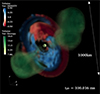 |
Fig. 1. 3D entropy plot for MHD jets (green region) at tpb = 100 ms. The red and blue region around the center is the normalized density deviation from the angle-averaged density on the equatorial plane. The central light yellow sphere is the PNS. |
The central PNS is strongly magnetized, with the PNS surface magnetic field strength reaching several times 1014 Gauss, and high rotation rates of several 100 rad s−1 (see Fig. 3 in Shibagaki et al. 2024). Consequently, the associated Maxwell stress decelerates the PNS rotation. In our model, the average angular velocity of the PNS starts to decrease around tpb ∼ 220 ms, and it vanishes at around tpb ∼ 350 ms.
The upper panel of Fig. 2 shows the plus and cross modes of the GW strains, h+ and h×, respectively, observed along the initial rotational axis, i.e., the direction of the north pole at a source distance of 10 kpc. The lower panel shows its V-mode spectrogram. We find the coherent large V-mode amplitude at tpb < 230 ms, which indicates strong circular polarization of the GW. Following Bugli et al. (2023), we compared this blue region in Fig. 2 to twice the maximum rotation frequency. As was indicated by Bugli et al. (2023) for the usual characteristic strain, we confirm here that for tpb < 230 ms, this blue region is always below twice the maximum rotation frequency, indicating that this feature originates from rotation. The moment-of-inertia–weighted average rotation rate of the PNS decreases rapidly at 220 ms < tpb < 340 ms, after which the PNS hardly rotates at all (Shibagaki et al. 2024). The V-mode amplitude is in a quiescent phase during 220 ms < tpb < 400 ms and irregularly shows both positive and negative values afterward. This is a clear indication that the V-mode amplitude does not stem from the rotational effect after tpb ∼ 220 ms alone.
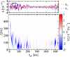 |
Fig. 2. GW strains of plus (solid red) and cross (dashed blue) modes (top) and spectrogram of its V-mode power spectrum (bottom) seen along the pole at a source distance of 10 kpc. |
In Fig. 3 we compare the spectra of the characteristic GW strains seen from the pole at a distance of 10 kpc for the I and V modes (see Appendix A for details) with the achieved O4 and target O5 sensitivity curves of LIGO (Abbott et al. 2022; Effler et al. 2025), Virgo (LIGO Scientific Collaboration 2025; Abbott et al. 2022), and KAGRA (Abbott et al. 2022; Enomoto & Komori 2019). Following Shibagaki et al. (2021), we calculated the sensitivity curves of the GW detectors for the V mode by assuming that two co-located detectors measure the GW plus and cross modes, respectively, and that the detector noises are Gaussian. Figure 3 shows that the I- and V-mode characteristic GW strains peak at ∼90 Hz. In this idealized situation, the signal-to-noise ratios of the GW peaks for the upcoming O5 run are expected to fall between the achieved O4 and target O5 levels, reaching ∼50−70 for the most sensitive detectors.
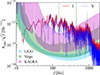 |
Fig. 3. Amplitude spectral densities of the I-mode (solid red) and V-mode (dotted blue) GW strains for a polar observer at 10 kpc. We also show the shaded sensitivity bands of current detectors: LIGO (light blue), Virgo (green), and KAGRA (magenta), bounded by the achieved O4 and target O5 sensitivities (dashed). |
To identify the origin of the coherent V-mode GW power spectrum at tpb < 230 ms shown in Fig. 2, we performed a mode analysis of the density on the equatorial plane, ρm(t, ϖ) = ∫02πρ(t, ϖ, ϕ, z = 0)cos(mϕ)dϕ. Figure 4 shows the m = 1 mode amplitude relative to the m = 0 mode amplitude (ρ1/ρ0) in the spacetime diagram. The largest relative amplitude is obtained at tpb ∼ 100 ms. This is also evident in the density deviation of Fig. 1 (red and blue disk). The regular appearance of alternating red and blue bands in Fig. 4 indicates that a density pattern rotates simultaneously with a given mode modulation. The finite slope of the red and blue bands refers to a nonvanishing radial velocity of the density pattern. The positive slope of the numerous bands, as shown in Fig. 4, indicates that the associated density patterns propagate outward. This is a characteristic feature of the low-T/|W| instability, which generates a quasi-periodic GW (e.g., Shibagaki et al. 2021). We note that this is not due to the spiral SASI because our model explodes almost without forming a standing shock. As shown in the previous studies (e.g., Takiwaki et al. 2021), the GW excited by the low-T/|W| instability appears at approximately twice the local angular velocity of the fluid. In our model, the ∼90 Hz GW signal corresponds to a region at a cylindrical radius of ∼50 km, where the angular velocity is ∼45 Hz (see Appendix B for a more detailed analysis).
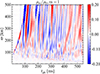 |
Fig. 4. Color map of the normalized m = 1 mode amplitude for the density deviation ρm/ρ0 as a function of time and cylindrical radius. |
The white region in the upper left corner of Fig. 4 corresponds to the outside of the shock surface, so the boundary between this white region and the red or blue region corresponds to the shock radius. After tpb ∼ 100 ms, the speed of the shock expansion and the propagation speed of the density pattern are comparable, such that the density pattern cannot reach the shock radius. This indicates that the advective-acoustic cycle, a mechanism that drives the SASI (Foglizzo & Tagger 2000; Scheck et al. 2008), is not involved in the generation of these density patterns after tpb ∼ 100 ms.
3. Conclusions
We investigated circular polarization of GWs from 3D GRMHD simulations of a magnetorotational supernova model (Shibagaki et al. 2024). Strong circular polarization emerges along the initial rotation axis during the early post-bounce phase (up to tpb ∼ 230 ms). This feature is associated with rotationally induced nonaxisymmetric deformations, in particular, the development of the low-T/|W| instability and spiral arm structures (e.g., Ott et al. 2005; Shibagaki et al. 2021).
The characteristic GW spectra are found to peak around 90 Hz, which can be interpreted as twice the local angular velocity of the fluid in the region where Ω ∼ 45 Hz at a cylindrical radius of ∼50 km. This interpretation is consistent with the theoretical expectation that the low-T/|W| instability excites GWs near twice the rotation frequency (e.g., Takiwaki et al. 2021). The frequency range of ∼90 Hz falls within the sensitivity bands of current ground-based detectors such as Advanced LIGO, Advanced Virgo, and KAGRA, suggesting a potential for detectability under idealized noise assumptions.
These results highlight the potential of GW polarization measurements as a diagnostic tool for probing the CCSN explosion mechanism and the dynamical PNS evolution. While previous studies mainly associated strong circular polarization with rapidly rotating nonmagnetized collapses (Hayama et al. 2016; Shibagaki et al. 2021), our findings have demonstrated that models that launch MHD jets can also exhibit distinct polarization signatures. Importantly, the circularly polarized GWs identified here originate predominantly from the low-T/|W| instabilities and nonaxisymmetric motions around the PNS surface and are not directly generated by the MHD jets themselves. This distinction suggests that future detector networks, with enhanced polarization analysis capabilities, can exploit these features to distinguish between different explosion scenarios.
Several limitations of this work should be mentioned. Our conclusions are based on a single progenitor model of a zero-age main-sequence mass of 20 M⊙ with rapid rotation and a strong magnetic field. A systematic exploration of the progenitor diversity, including variations in rotation rates and magnetic field strengths, will be necessary to confirm the robustness of these findings. Moreover, the role of turbulence and nonlinear instabilities requires further study, particularly with respect to numerical resolution and diffusion effects (Mösta et al. 2014; Bugli et al. 2021). Finally, a more realistic evaluation of detectability will require incorporating detector noise properties and advanced data-analysis strategies.
In summary, we identified circularly polarized GW emission as a robust feature of magnetorotational explosions and provided a pathway toward using polarization as a probe of the central engine in energetic core-collapse events. Our findings serve as a milestone for future studies, including broader parameter surveys and predictions for third-generation detectors. These will be crucial to fully exploit the diagnostic potential of GW polarization in multimessenger astrophysics.
Acknowledgments
Numerical computations were carried out on Cray XC50 at the Center for Computational Astrophysics, National Astronomical Observatory of Japan and on Cray XC40 at YITP in Kyoto University. This work was supported by JSPS KAKENHI Grant Number (JP17H06364, JP22H01223, JP21H01088, JP23H01199, JP23K03400, JP23K22494, JP24K00631, and JP26K07093), MEXT as “Program for Promoting researches on the Supercomputer Fugaku” (Structure and Evolution of the Universe Unraveled by Fusion of Simulation and AI; Grant Number JPMXP1020230406), and JICFuS. The authors acknowledge support from the program Excellence Initiative–Research University of the University of Wrocław of the Ministry of Education and Science and the Scultetus Visiting Scientist Program of the Center for Advanced Systems Understanding (S.S.) and the Polish National Science Centre (NCN) under grant number 2023/49/B/ST9/03941 (S.S. and T.F.) as well as by the WCSS Wrocław Centre for Scientific Computing and Networking (T.F.).
References
- Abbott, B. P., Abbott, R., Abbott, T. D., et al. 2019, Phys. Rev. X, 9, 031040 [Google Scholar]
- Abbott, R., Abbott, T. D., Abraham, S., et al. 2021, Phys. Rev. X, 11, 021053 [Google Scholar]
- Abbott, R., et al. 2022, Noise Curves Used for Simulations in the Update of the Observing Scenarios Paper, Tech. Rep. LIGO-T2000012-v2, LIGO Scientific Collaboration [Google Scholar]
- Abbott, R., Abbott, T. D., Acernese, F., et al. 2023, Phys. Rev. X, 13, 041039 [Google Scholar]
- Abdikamalov, E., Pagliaroli, G., & Radice, D. 2022, in Handbook of Gravitational Wave Astronomy, eds. C. Bambi, S. Katsanevas, & K. D. Kokkotas (Singapore: Springer Singapore), 1 [Google Scholar]
- Andresen, H., Müller, B., Müller, E., & Janka, H. T. 2017, MNRAS, 468, 2032 [NASA ADS] [CrossRef] [Google Scholar]
- Baumgarte, T. W., & Shapiro, S. L. 1999, Phys. Rev. D, 59, 024007 [Google Scholar]
- Blondin, J. M., Mezzacappa, A., & DeMarino, C. 2003, ApJ, 584, 971 [NASA ADS] [CrossRef] [Google Scholar]
- Bugli, M., Guilet, J., & Obergaulinger, M. 2021, MNRAS, 507, 443 [NASA ADS] [CrossRef] [Google Scholar]
- Bugli, M., Guilet, J., Foglizzo, T., & Obergaulinger, M. 2023, MNRAS, 520, 5622 [NASA ADS] [CrossRef] [Google Scholar]
- Burrows, A., & Vartanyan, D. 2021, Nature, 589, 29 [CrossRef] [PubMed] [Google Scholar]
- Choi, L., Burrows, A., & Vartanyan, D. 2024, ApJ, 975, 12 [Google Scholar]
- Dimmelmeier, H., Ott, C. D., Marek, A., & Janka, H.-T. 2008, Phys. Rev. D, 78, 064056 [Google Scholar]
- Effler, A., Fritschel, P., Kabagoz, B., & Kuns, K. 2025, A+/O5 Strain Curve Projections, Tech. Rep. LIGO-T2500310-v2, LIGO Scientific Collaboration [Google Scholar]
- Enomoto, Y., Komori, K., et al. 2019, Latest Estimated Sensitivity of KAGRA (v201708), Tech. Rep. JGW-T1707038-v9, KAGRA Collaboration [Google Scholar]
- Foglizzo, T., & Tagger, M. 2000, A&A, 363, 174 [NASA ADS] [Google Scholar]
- Hayama, K., Kuroda, T., Nakamura, K., & Yamada, S. 2016, Phys. Rev. Lett., 116, 151102 [Google Scholar]
- Hayama, K., Kuroda, T., Kotake, K., & Takiwaki, T. 2018, MNRAS, 477, L96 [Google Scholar]
- Janka, H.-T. 2025, Annu. Rev. Nucl. Part. Sci., 75, 425 [Google Scholar]
- Janka, H.-T., Melson, T., & Summa, A. 2016, Annu. Rev. Nucl. Part. Sci., 66, 341 [Google Scholar]
- Jerkstrand, A., Milisavljevic, D., & Müller, B. 2026, in Encyclopedia of Astrophysics First Edition, ed. I. Mandel (Oxford: Elsevier), 639 [Google Scholar]
- Kalogera, V., Sathyaprakash, B. S., Bailes, M., et al. 2021, ArXiv e-prints [arXiv:2111.06990] [Google Scholar]
- Kazeroni, R., Guilet, J., & Foglizzo, T. 2017, MNRAS, 471, 914 [NASA ADS] [CrossRef] [Google Scholar]
- Kotake, K., & Kuroda, T. 2017, in Handbook of Supernovae, eds. A. W. Alsabti, & P. Murdin (Springer International Publishing), 1671 [Google Scholar]
- Kotake, K., Sumiyoshi, K., Yamada, S., et al. 2012, Progr. Theor. Exp. Phys., 2012, 010000 [Google Scholar]
- Kuroda, T. 2021, ApJ, 906, 128 [Google Scholar]
- Kuroda, T., & Shibata, M. 2024, MNRAS, 533, L107 [Google Scholar]
- Kuroda, T., Takiwaki, T., & Kotake, K. 2014, Phys. Rev. D, 89, 044011 [CrossRef] [Google Scholar]
- Kuroda, T., Kawaguchi, K., & Shibata, M. 2025, MNRAS, 541, 1649 [Google Scholar]
- LIGO Scientific Collaboration, Virgo Collaboration,& KAGRA Collaboration 2025, https://doi.org/10.5281/zenodo.17151534 [Google Scholar]
- Marronetti, P., Tichy, W., Brügmann, B., González, J., & Sperhake, U. 2008, Phys. Rev. D, 77, 064010 [Google Scholar]
- Mezzacappa, A., Endeve, E., Messer, O. E. B., & Bruenn, S. W. 2020, Liv. Rev. Comput. Astrophys., 6, 4 [CrossRef] [Google Scholar]
- Mezzacappa, A., Marronetti, P., Landfield, R. E., et al. 2023, Phys. Rev. D, 107, 043008 [NASA ADS] [CrossRef] [Google Scholar]
- Mösta, P., Richers, S., Ott, C. D., et al. 2014, ApJ, 785, L29 [CrossRef] [Google Scholar]
- Müller, B. 2016, PASA, 33, e048 [Google Scholar]
- Müller, B. 2025, in Supernova Simulations, eds. C. Bambi, Y. Mizuno, S. Shashank, & F. Yuan (Singapore: Springer Nature Singapore), 663 [Google Scholar]
- Nakamura, K., Takiwaki, T., Matsumoto, J., & Kotake, K. 2025, MNRAS, 536, 280 [Google Scholar]
- Nomoto, K., Tominaga, N., Umeda, H., Kobayashi, C., & Maeda, K. 2006, Nucl. Phys. A, 777, 424 [CrossRef] [Google Scholar]
- Obergaulinger, M., & Aloy, M. Á. 2020, MNRAS, 492, 4613 [Google Scholar]
- Obergaulinger, M., & Aloy, M. Á. 2022, MNRAS, 512, 2489 [NASA ADS] [CrossRef] [Google Scholar]
- Ott, C. D., Ou, S., Tohline, J. E., & Burrows, A. 2005, ApJ, 625, L119 [NASA ADS] [CrossRef] [Google Scholar]
- Pajkos, M. A., VanCamp, S. J., Pan, K.-C., et al. 2023, ApJ, 959, 21 [Google Scholar]
- Powell, J., & Müller, B. 2019, MNRAS, 487, 1178 [NASA ADS] [CrossRef] [Google Scholar]
- Radice, D., Abdikamalov, E., Ott, C. D., et al. 2018, J. Phys. G Nucl. Phys., 45, 053003 [Google Scholar]
- Rampp, M., Mueller, E., & Ruffert, M. 1998, A&A, 332, 969 [Google Scholar]
- Scheck, L., Janka, H.-T., Foglizzo, T., & Kifonidis, K. 2008, A&A, 477, 931 [NASA ADS] [CrossRef] [EDP Sciences] [Google Scholar]
- Schnauck, S. C., Shankar, S., Mösta, P., Haas, R., & Schnetter, E. 2026, MNRAS, 546, stag056 [Google Scholar]
- Seto, N., & Taruya, A. 2007, Phys. Rev. Lett., 99, 121101 [Google Scholar]
- Shibagaki, S., Kuroda, T., Kotake, K., & Takiwaki, T. 2020, MNRAS, 493, L138 [Google Scholar]
- Shibagaki, S., Kuroda, T., Kotake, K., & Takiwaki, T. 2021, MNRAS, 502, 3066 [NASA ADS] [CrossRef] [Google Scholar]
- Shibagaki, S., Kuroda, T., Kotake, K., Takiwaki, T., & Fischer, T. 2024, MNRAS, 531, 3732 [NASA ADS] [CrossRef] [Google Scholar]
- Shibata, M., & Nakamura, T. 1995, Phys. Rev. D, 52, 5428 [Google Scholar]
- Shibata, M., & Sekiguchi, Y.-I. 2003, Phys. Rev. D, 68, 104020 [Google Scholar]
- Sotani, H., Takiwaki, T., & Togashi, H. 2021, Phys. Rev. D, 104, 123009 [NASA ADS] [CrossRef] [Google Scholar]
- Stritzinger, M. D., Taddia, F., Burns, C. R., et al. 2018, A&A, 609, A135 [NASA ADS] [CrossRef] [EDP Sciences] [Google Scholar]
- Szczepańczyk, M., & Zanolin, M. 2022, Galaxies, 10, 70 [Google Scholar]
- Szczepańczyk, M. J., Zheng, Y., Antelis, J. M., et al. 2024, Phys. Rev. D, 110, 042007 [Google Scholar]
- Takiwaki, T., & Kotake, K. 2018, MNRAS, 475, L91 [NASA ADS] [CrossRef] [Google Scholar]
- Takiwaki, T., Kotake, K., & Foglizzo, T. 2021, MNRAS, 508, 966 [NASA ADS] [CrossRef] [Google Scholar]
- Torres-Forné, A., Cerdá-Durán, P., Obergaulinger, M., Müller, B., & Font, J. A. 2019, Phys. Rev. Lett., 123, 051102 [CrossRef] [Google Scholar]
- Torres-Forné, A., Cerdá-Durán, P., Obergaulinger, M., Müller, B., & Font, J. A. 2021, Phys. Rev. Lett., 127, 239901 [CrossRef] [Google Scholar]
- Walk, L., Foglizzo, T., & Tamborra, I. 2023, Phys. Rev. D, 107, 063014 [NASA ADS] [CrossRef] [Google Scholar]
- Woosley, S. E., & Heger, A. 2007, Phys. Rep., 442, 269 [Google Scholar]
- Yamada, S., Nagakura, H., Akaho, R., et al. 2024, Proc. Jpn. Acad. Ser. B, 100, 190 [Google Scholar]
Appendix A: Numerical setup
A.1. Simulation code and initial condition
We carried out our simulations with the 3D GR neutrino-radiation ideal MHD code developed by Kuroda (2021). The spacetime metric is evolved using the Baumgarte–Shapiro–Shibata–Nakamura formulation (see, e.g., Shibata & Nakamura 1995; Baumgarte & Shapiro 1999; Marronetti et al. 2008) on a fixed Cartesian mesh. As in Kuroda (2021), the grid resolution is chosen such that the finest level near the center reaches Δx = 458 m. The computational domain covers a region of 1.5 × 10⁴ km in radius, with 10 nested refinement levels in a 2:1 ratio. Each refinement box contains 643 zones.
As the progenitor, we use the solar-metallicity 20 M⊙ model “s20a28n” from Woosley & Heger (2007), which is commonly employed in CCSN studies. A cylindrical rotation law is imposed, setting the initial angular momentum distribution as utuϕ = ϖ02 (Ω0 − Ω), where ut is the temporal component of the four-velocity, uϕ ≡ ϖ2Ω with 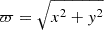 , and ϖ0 is taken to be 108 cm.
The initial magnetic field is specified through a purely toroidal vector potential, 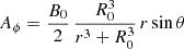 , Ar = Aθ = 0, which yields an approximately uniform vertical field inside r < R0 and a dipolar field outside. In this study we set R0 = 108 cm. For the present work we analyze the model with
 ![Mathematical equation: $ (\Omega_0\,[\mathrm{rad\,s^{-1}}], B_0[\mathrm{G}]/\sqrt{4\pi}) = (2.0, 10^{12}) $](/articles/aa/full_html/2026/07/aa59979-26/aa59979-26-eq3.gif) , denoted as R20B12 following Shibagaki et al. (2024).
, denoted as R20B12 following Shibagaki et al. (2024).
A.2. Gravitational wave analysis
We extract the GWs with a standard quadrupole formula (Shibata & Sekiguchi 2003; Kuroda et al. 2014). To investigate the spectral evolution of the circularly polarized component of the GWs, we evaluate the Stokes I and V parameters (Seto & Taruya 2007; Hayama et al. 2016),
 (A.1)
(A.1)
 (A.2)
(A.2)
where  is the Fourier amplitude of the GW strain, h, and Δf is the smallest frequency width of the Fourier transform, i.e., the inverse of the integration time for the Fourier transform. The hR and hL are the right-handed and left-handed polarization modes, which are defined by
  and
and  . The Stokes I parameter indicates the total power spectrum, while the Stokes V parameter represents the power spectrum of the difference between its clockwise circularly polarized component and counterclockwise one. For the discussion of the detectability of these modes, it is convenient to define the characteristic GW strain for the I and V modes,
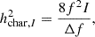 (A.3)
(A.3)
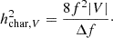 (A.4)
(A.4)
These quantities are defined so that hchar, I becomes identical to the well-known characteristic GW strain (Shibagaki et al. 2021).
To perform time-frequency analysis of these modes, we perform a short-time Fourier transform of the GW strain with the Hann window:
 (A.5)
(A.5)
 (A.6)
(A.6)
Replacing  in Eqs. (A.1) and (A.2) with H in Eq. (A.5), we can obtain time-frequency spectrograms of the I mode, I(t, f), and the V mode, V(t, f). In this study, we use 20 ms of Δt.
Appendix B: Emission Region
For further analysis of the GW emission regions, we compute V-mode spectrograms observed from the pole using quadrupole moments of limited spatial domains (|z|< z0). Figure B.1 shows the V-mode spectrograms normalized by the total V-mode amplitude. z0 is denoted on the upper right corner. To extract important parts of the spectrograms, we only plot regions where the total V-mode spectrogram is larger than 10−46. Looking at tpb < 230 ms, ∼60% of the V-mode amplitude is generated in the region of |z|< 100 km and ∼80% in the region of |z|< 200 km. This is consistent with our interpretation that the GWs are generated by not only the deformed PNS but also extended spiral arms driven by the low-T/|W| instability.
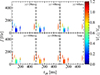 |
Fig. B.1. Relative contributions from each rectangular box defined by |z|< z0 to the total V-mode GW spectrogram (seen from the pole). We color only the t − f domains with |Vtot|> 10−46. The value of z0 is shown in the upper right corner of each panel. As a reference, the bottom right panel shows the total V-mode GW spectrogram. |
All Figures
|
Fig. 1. 3D entropy plot for MHD jets (green region) at tpb = 100 ms. The red and blue region around the center is the normalized density deviation from the angle-averaged density on the equatorial plane. The central light yellow sphere is the PNS. |
| In the text | |
|
Fig. 2. GW strains of plus (solid red) and cross (dashed blue) modes (top) and spectrogram of its V-mode power spectrum (bottom) seen along the pole at a source distance of 10 kpc. |
| In the text | |
|
Fig. 3. Amplitude spectral densities of the I-mode (solid red) and V-mode (dotted blue) GW strains for a polar observer at 10 kpc. We also show the shaded sensitivity bands of current detectors: LIGO (light blue), Virgo (green), and KAGRA (magenta), bounded by the achieved O4 and target O5 sensitivities (dashed). |
| In the text | |
|
Fig. 4. Color map of the normalized m = 1 mode amplitude for the density deviation ρm/ρ0 as a function of time and cylindrical radius. |
| In the text | |
|
Fig. B.1. Relative contributions from each rectangular box defined by |z|< z0 to the total V-mode GW spectrogram (seen from the pole). We color only the t − f domains with |Vtot|> 10−46. The value of z0 is shown in the upper right corner of each panel. As a reference, the bottom right panel shows the total V-mode GW spectrogram. |
| In the text | |
Current usage metrics show cumulative count of Article Views (full-text article views including HTML views, PDF and ePub downloads, according to the available data) and Abstracts Views on Vision4Press platform.
Data correspond to usage on the plateform after 2015. The current usage metrics is available 48-96 hours after online publication and is updated daily on week days.
Initial download of the metrics may take a while.