


| Issue |
A&A
Volume 711, July 2026
|
|
|---|---|---|
| Article Number | A70 | |
| Number of page(s) | 16 | |
| Section | Catalogs and data | |
| DOI | https://doi.org/10.1051/0004-6361/202659763 | |
| Published online | 06 July 2026 | |
Hot carbon-dominated, magnetic, and metal-polluted white dwarfs: Spectroscopic insights from a Gaia machine-learning-selected 500 pc sample
1
Departament de Física, Universitat Politècnica de Catalunya,
c/Esteve Terrades 5,
08860
Castelldefels,
Spain
2
Institut d’Estudis Espacials de Catalunya, Esteve Terrades,
1, Edifici RDIT, Campus PMT-UPC,
08860
Castelldefels,
Spain
★ Corresponding author: This email address is being protected from spambots. You need JavaScript enabled to view it.
Received:
9
March
2026
Accepted:
9
May
2026
Abstract
Context. The latest Gaia data release provides astrometric measurements for 1.8 billion sources and low-resolution spectra for 220 million sources, including approximately 100 000 white dwarfs. Although useful for pre-classification, Gaia spectra lack the resolution required for accurate spectral typing and reliable parameter determination, motivating dedicated spectroscopic follow-up observations.
Aims. We assessed the reliability of machine-learning spectral classifications derived from Gaia spectra by comparing them with medium-resolution spectroscopy. We determined the nature of objects classified as ‘massive helium-rich (DB)’ white dwarfs by automated methods, and characterised the properties of warm and hot carbon-dominated (DQ) white dwarfs, as well as magnetic and metal-polluted objects.
Methods. We observed 255 white dwarfs along the Gaia B- and Q-branches with the Gran Telescopio Canarias, equipped with the OSIRIS instrument (R≃1000). We assigned spectral types through visual inspection and compared them with machine-learning classifications applied to Gaia spectra. For objects labelled as ‘massive DBs’, we independently determined their atmospheric spectral compositions. We identified magnetic white dwarfs via Zeeman splitting and estimated first-order magnetic field strengths when possible.
Results. Machine-learning classifications are highly accurate (>90% for spectral types included in their training sets), despite the low resolution of Gaia spectra. We determine that objects classified as ‘massive DBs’ are largely magnetic white dwarfs and warm DQs, with only five of 112 observed objects (4.46%) confirmed as genuine DBs. Warm DQs are found along the Gaia Q-branch and exhibit unusually high tangential velocities.
Conclusions. We provide spectral classifications for 255 white dwarfs and demonstrate that random forest algorithms reliably classify low-resolution Gaia spectra for the main spectral types. We also determine the nature of objects classified as ‘massive DBs’ and identify a large population of magnetic white dwarfs and carbon-rich objects. We identify several rare subtypes including two DAB, one DBAZ, one DZAB, two DZBA, 14 DAH, one DAQ, one DQZA, four hot, and 29 warm DQ stars, along with 63 magnetic white dwarfs. The location and kinematics of warm DQs are consistent with previous studies, supporting their proposed origin as merger remnants.
Key words: catalogs / stars: atmospheres / Hertzsprung-Russell and C-M diagrams / white dwarfs
© The Authors 2026
 Open Access article, published by EDP Sciences, under the terms of the Creative Commons Attribution License (https://creativecommons.org/licenses/by/4.0), which permits unrestricted use, distribution, and reproduction in any medium, provided the original work is properly cited.
This article is published in open access under the Subscribe to Open model. This email address is being protected from spambots. You need JavaScript enabled to view it. to support open access publication.
1 Introduction
White dwarfs, the degenerate cores of stars with initial masses lower than 8–10 M⊙, are the most common stellar remnant in the Galaxy (Althaus et al. 2010). Spectroscopic observations provide information on their atmospheric composition, allowing classification into different spectral types and subtypes based on the most prominent spectral features. As such, a white dwarf that shows Balmer lines is classified as a DA, another that shows He I features is classified as a DB, and a spectrum with metallic lines as well as magnetic Zeeman splitting is classified as a DZH white dwarf. A more detailed description of the classification of white dwarfs is given in Sion et al. (1983).
An accurate spectral classification of white dwarfs is essential not only for an accurate determination of the white dwarf parameters (Bergeron et al. 2019; Tremblay et al. 2019a), but also for understanding the spectral evolution of white dwarfs (see Bédard 2024 and the references therein). Furthermore, features such as the high ratio of DQs (white dwarfs displaying carbon features) inside the Q-branch (Tremblay et al. 2019b), or the presence of carbon in hydrogen-deficient atmospheres, proposed as a possible explanation for the Gaia colour-magnitude bifurcation (Camisassa et al. 2023; Blouin et al. 2023), depend on correct spectral identification. This is also true for processes such as convective mixing or dilution in white dwarfs (Blouin et al. 2019; Cunningham et al. 2020). Metal-polluted DZ white dwarfs, in turn, allow us to investigate the origin and composition of the accreted material, as determined by their abundances (Zuckerman et al. 2007; Farihi et al. 2010).
In recent years, the Gaia mission (Gaia Collaboration 2016) has sparked a revolution in the astronomical community by providing astrometric and photometric measurements for 1.8 billion sources, as well as spectral information for 220 million objects (De Angeli et al. 2023), including more than 100 000 white dwarfs. The spectrophotometric data, however, have a modest resolving power (30 ≲ R ≲ 100; Carrasco et al. 2021), which limits their diagnostic capability. Despite the remarkable success of automated classification techniques applied to these data (e.g. García-Zamora et al. 2023; Vincent et al. 2023, 2024; Pérez-Couto et al. 2024; García-Zamora et al. 2025), the reliability of such classifications for rare or spectroscopically complex subtypes is lower and more uncertain, as these classes are typically under-represented in training sets (García-Zamora et al. 2023; García-Zamora et al. 2025). In particular, objects located along the Gaia B- and Q-branches may present atmospheric compositions or even magnetic features that are difficult to disentangle at Gaia resolution, potentially leading to misclassifications that propagate into population studies.
Motivated by the need to assess the robustness of automated classifications and to clarify the nature of peculiar sub-groups – such as the massive objects classified as DB in García-Zamora et al. (2025) and Vincent et al. (2024) – we conducted a series of spectroscopic follow-up campaigns using the Gran Telescopio Canarias (GTC). Its 10.4 m aperture enables efficient spectroscopy of intrinsically faint white dwarfs with moderate exposure times. We selected 321 white dwarfs within 500 pc of the Sun as targets, of which 255 were observed and subsequently analysed. The selected sample is well suited to testing the reliability of classification and investigate peculiar subtypes in critical regions of the Gaia colour–magnitude diagram.
This paper is organised as follows. In Section 2, we describe the selection of the white dwarf sample and the details of the observational campaigns. Section 3 presents the visual spectral classification of the targets based on medium-resolution spectroscopy. In Section 4, we present a general analysis of the sample, including a comparison with machine-learning classifications derived from Gaia spectra, as well as a detailed discussion of objects along the Q-branch, the DQ population, and magnetic white dwarfs. Finally, in Section 5 we summarise our main results and outline future perspectives.
Log of observations.
2 White dwarf sample and observing campaigns
Since the 2023B observing semester at the GTC (September 2023–February 2024), we conducted four observational campaigns in semesters 2023B, 2024B, 2025A, and 2025B with different scopes and aims. In all cases, we limited the declination (Dec > – 15 deg) and apparent magnitude (G ≤ 19.2 mag) to avoid excessively low sky altitudes and excessively long exposure times, respectively. Table 1 shows a log of the observations.
The 2023B and 2024B campaigns aimed to ascertain the spectral classifications obtained through the random forest algorithms described in García-Zamora et al. (2023); García-Zamora et al. (2025). More specifically, the campaigns evaluated the high precision (true positives to all positives ratio) obtained for the DB, DQ, DO, and DZ spectral types, as well as the correct classification of the three magnetic DAH white dwarfs identified in these two studies. For this reason, all selected targets belonged to these pre-classified spectral types. A total of 183 objects were intended for observation during these two semesters (see Table 1). The comparison between the predicted and observed types for these objects allowed us to test the capabilities of automatic classification algorithms (see Section 4.1).
In contrast, the 2025A and 2025B campaigns focused on uncovering the true nature of a subpopulation of approximately 350 white dwarfs classified as DB by the machine-learning algorithms of García-Zamora et al. (2025); Vincent et al. (2024). We refer to these objects as the ‘massive DB’ subpopulation since they are located below the M ≥ 0.95 M⊙ DB cooling track of Camisassa et al. (2019) in the Gaia Hertzsprung-Russell (HR) diagram, on and above the Q-branch, which we define as the region limited by the 0.83 M⊙ and 1.29 M⊙ DA cooling tracks from Camisassa et al. (2019) and the CO-core crystallisation onset (top track) and 80% mass crystallisation (bottom track) curves from Camisassa et al. (2024). It should be noted that this subpopulation has not been identified in other spectroscopic works (Genest-Beaulieu & Bergeron 2019; Bergeron et al. 2011) or in the volume-limited Gaia samples of Hollands et al. (2018), García-Zamora et al. (2023), and O’Brien et al. (2023). We selected a total of 138 objects from the García-Zamora et al. (2025) and Vincent et al. (2024) catalogues for observations (see Table 1). Sect. 4.2 and Table 6 provide a detailed account of these findings.
Of the 321 intended objects, we observed 255 (79.44%; Table 1). Of these, 213 are new, while the remaining 42 have been observed in recent papers (see Table 2). The observations were carried out under any lunar brightness with a maximum seeing of 1.5″ and a maximum airmass of 1.5. All four campaigns requested long-slit spectroscopy with the Optical System for Imaging and low-Intermediate-Resolution Integrated Spectroscopy (OSIRIS; see Cepa et al. 2013) instrument equipped with the R1000B grism and a 0.6″ slit width. This resulted in medium resolution spectra (R~1000) covering the 3600 ≲ λ ≲ 7800 Å wavelength range. Under the requested sky and atmospheric conditions described above, we defined exposure times to achieve a signal-to-noise ratio (S/N) of ~35 at Hβ for each spectrum in exposures of less than one hour. However, since the observations were performed in service mode, these conditions were not always met, which resulted in lower S/N spectra in some cases. The achieved S/N was sufficient to distinguish the spectral features of the observed white dwarfs, enabling a correct spectral classification. We reduced the GTC spectra using the pamela (Marsh 2014) and molly (Marsh 2019)1 packages.
Fig. 1 shows the Gaia HR diagram of the observed targets from each campaign, superimposed on the 100 pc Gaia white dwarf sample from Jiménez-Esteban et al. (2023).
Objects reported in recent papers.
Excerpt from the observed sample.
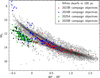 |
Fig. 1 Gaia HR diagram of the targets observed at the GTC during the 2023B, 2024B, 2025A, and 2025B semesters, superimposed on the Gaia 100 pc white dwarf sample of Jiménez-Esteban et al. (2023). |
3 Visual spectral classification
In this section, we present a breakdown of the spectral types and subtypes assigned through visual inspection of the GTC spectra. This includes both predicted and unexpected subtype characteristics, as well as classifications that were not included in the initial training sets and therefore could not be predicted by the algorithm, such as cataclysmic variables (CVs). We present selected spectra of objects described in this section in Appendix B. Table 3 shows an excerpt from the complete observed sample, while the full catalogue is available from the CDS.
3.1 DAs
In total, we identify 26 DA white dwarfs. Of these, three are DAH candidates correctly classified as such by our random forest algorithm, 11 are DAHs classified as ‘massive DB’ white dwarfs, and the remaining 12 are DAs misclassified as non-DAs. The misclassification of these objects was unexpected, as the DA versus non-DA validation tests in García-Zamora et al. (2023); García-Zamora et al. (2025) show very good performance.
Pure DAs. We identify nine of our targets as pure DAs, displaying only Balmer lines. These include J0239+3733, J0313–0131, J0641+2018 (classified as a DZs and a DQ, respectively), as well as J0016+5251, J0628+0622, J0726–0912, J1405–0932, J1643+6627, and J1810+1240, which were flagged as belonging to the ‘massive DB’ subpopulation. Figure B.1 of Appendix B shows an example spectrum.
DABs. Objects J0050+3138 and J1747+1701 display Balmer lines as well as helium features, namely the He I λλ = 4471, 5876 Å spectral lines. We therefore classify their spectra (see Fig. B.1 in Appendix B) as DAB.
DAHs. Fourteen of the identified DAs show magnetic Zeeman splitting, which is especially evident around the Hα and Hβ lines. They therefore belong to the DAH subtype. Fig. B.1 in Appendix B shows an example spectrum, while we estimate the strength of their magnetic fields in Sect. 4.9.1.
DAQs. The DAQ class is a recently discovered (Hollands et al. 2020), extremely rare (with only 26 known objects) class of white dwarfs, with spectra displaying Balmer and C I lines. They are characterised by high masses and peculiar kinematics (Hollands et al. 2020; Kilic et al. 2024, 2025), properties shared with warm and hot DQs (see Sect. 4.7 for a discussion and analysis of DQs, DQAs, and warm and hot DQs). This is because they belong to the same subpopulation. Kilic et al. (2024) show that warm DQs display a range of hydrogen atmospheric abundances: DAQs form the H-rich end, while DQAs and DQs are found at the H-deficient end (see also Fig. 7 of Kilic et al. 2025 and Fig. 28 of Kilic et al. 2026).
We visually identify one DAQ, J0325+2540. This object, also classified as such by Kilic et al. (2025), is a hot white dwarf found in the Q-branch. Figure B.1 of Appendix B shows its spectrum.
3.2 DBs
Among the objects observationally classified as DB, we identify nine pure DBs, eight DBAs, and one DBAZ. Most of these objects are not part of the ‘massive DB’ subpopulation, with only five belonging to it (three DBs and two DBAs).
Figure B.1 of Appendix B show two example spectra of a massive DB and a massive DBA.
Pure DBs. We identify nine pure DBs in our observational campaigns. Most of them are located in the −0.10 ≤ GBP − GRP ≤ 0.01 colour range (top-right panel of Fig. A.1 in Appendix A). The exceptions are J0622+6935, J0903–1311, and J1832+0856, which are located in the −0.40 ≤ GBP − GRP ≤ −0.30 colour range. Interestingly, these objects belong to the ‘massive DB’ subpopulation.
DBAs. We identify eight DBAs with both He I and Balmer lines of lesser intensity. Of these, one also displays the H and K Ca II lines and is treated in the following subsection. All white dwarfs are in the −0.07 ≤ GBP − GRP ≤ 0.03 colour range, except J0646+1151, with GBP − GRP = −0.11. Unlike Sect. 3.2, this outlier does not belong to the ‘massive DB’ subpopulation.
DBAZ. Among all the observationally classified DB white dwarfs in our sample, we also find a rare case of a DBAZ white dwarf. Only 39 such objects are listed in the Montreal White Dwarf Database2 (MWDD; see Dufour et al. 2017). This object, J0201+6221, displays helium and hydrogen features as well as the metallic Ca II H-K doublet lines in its spectrum. Fig. B.2 of Appendix B shows this spectrum.
3.3 DCs
We find 27 DC white dwarfs. Of these, three are cool DCs (0.43 ≤ GBP − GRP), while the remaining 24 are hot DCs (0.10 ≥ GBP − GRP). Fig. B.2 of Appendix B shows the spectrum of a hot DC.
3.4 DOs
We identify six DO white dwarfs. All are very hot objects (GBP − GRP < −0.40) and display the characteristic He II lines that define this spectral type. Additionally, all of them lack He I lines, except J0513+1147, which displays prominent absorption at λλ = 4471, 5876 Å, and J0536+5448, which displays a weak He I λ = 5876 Å line.
Pure DOs. Of the six identified DOs, two (J0513+1147 and J0536+5448) display exclusively helium spectral features. They are therefore classified as pure DOs. These are the only objects to display He I lines. Figure B.2 of Appendix B shows one of these spectra.
DOZs. Four of our DOs (J0447+0458, J0515+0728, J0519–0443, and J0602–1351) show C IV features most prominently around λλλ = 4441, 4658, 5470 Å, in addition to He II spectral lines, as well as a lack of He I lines. Such objects would be classified as DOQ but are instead designated as DOZs for historical reasons (see Footnote 3 in Bédard et al. 2022a). We follow this convention and assign the DOZ type to these objects. Figure B.2 of Appendix B shows one of these spectra.
3.5 DQs
We identify two distinct groups among the 47 visually identified DQs. On the one hand, there is the cool DQ subpopulation (Teff ≲ 10 000 K), which displays molecular C2 Swan bands in its spectra. On the other hand, there are the warm and hot DQ subpopulations (Teff ≳ 10 000 K), whose spectra are dominated by atomic lines of neutral C I and ionised C II, respectively. The limit between hot and warm DQs is not well defined, as the strength of the C I and C II spectral lines varies gradually with temperature rather than appearing and disappearing abruptly. Koester & Kepler (2019) arbitrarily sets Teff = 18 000 K as the temperature limit between hot and warm DQs.
Cool DQs. We identify 15 cool DQs. Of these, three (J0506+2030, J0722+6143, and J1942+3402) belong to the peculiar DQ subtype (DQpec, cool DQs in which the Swan bands appear slightly blue-shifted and with a more rounded appearance than in regular DQs; see Hall & Maxwell 2008 for further information). García-Zamora et al. (2023) correctly predicted all three as DQpecs. Figure B.2 of Appendix B shows example spectra of a cool DQ and a DQpec.
Warm DQs. We identify 28 warm DQs. Of these, 11 are pure warm DQs, displaying only carbon features, whereas 16 are warm DQAs that also display Balmer lines. One object is a warm DQZA with neutral oxygen features in addition to carbon and hydrogen. We note the absence of He I lines in all cases, in agreement with the results of Kilic et al. (2025). Figure B.3 in Appendix B shows sample spectra of warm DQ and DQA white dwarfs.
Hot DQs. Of the 170 ‘massive DB’ candidates, we visually identify four hot DQ candidates: J0034+7130, J0420+6450, J0446+7227, and J0642+0632. All four objects also display signatures of Zeeman splitting and are therefore classified as magnetic hot DQHs. Figure B.3 in Appendix B shows a sample spectrum.
DQZA. In J0328+5806, we identify O I spectral features in addition to CI and Balmer lines, which are especially evident at wavelengths λλλλ = 5330, 5436, 6158, 6456 Å. Figure B.3 of Appendix B shows the spectrum of this object.
Warm DQs with oxygen features are extremely rare. A literature search reveals that Liebert et al. (2003) reported two such cases, as did Gänsicke et al. (2010) and Kepler et al. (2015), while Kilic et al. (2025) identify an additional instance and a doubtful case. Figure B.3 of Appendix B shows the spectrum of this object.
3.6 DZs
We find 90 observed spectra of metal-polluted white dwarfs. The metals are varied, ranging from spectra showing only the Ca II H and K lines to those also displaying spectral lines of iron, magnesium, or sodium.
Pure DZs. Of the 90 DZs, 74 (82.2%) do not display additional subtype characteristics, showing only metallic lines. Fig. B.3 of Appendix B shows a pure DZ example spectrum.
DZAs. Seven other white dwarfs (J0410+0847, J0505+0048, J0543+3936, J0628+6636, J0709–1332, J1803+1634, and J2015+4742) show less intense hydrogen spectral features in addition to metals, in most cases only the Hα line. This combination places them in the DZA subtype. Figure B.4 of Appendix B shows an example.
DZAB. The spectrum of J0452–0214 shows He I spectral lines, in addition to metallic lines and hydrogen features. Since the hydrogen lines are more intense than the helium lines, we classify it as the rare DZAB subtype, of which only two such objects are listed in the MWDD. We show its spectrum in Fig. B.4 in Appendix B.
DZBA. Furthermore, we identify two additional objects, J0437+0051 and J0745+5551, that, like J0452–0214, show metallic lines, as well as HI and He I features. However, in these cases, the He lines are more intense. We therefore classify them as the DZBA type, of which only one other member (a magnetic DZBAH) is listed in the MWDD. Fig. B.4 of Appendix B shows the spectrum of J0745+5551.
DZHs. We identify six white dwarfs (J0342+2934, J0610–1402, J0738+7424, J0829–0818, J1543–0247, and J2357+2747) that show signatures of magnetic Zeeman splitting. This is particularly pronounced around the NaI doublet at λλ = 5890, 5895 Å, which becomes a triplet; the Mg I triplet at λλλ = 5167, 5173, 5184 Å, which splits into four components; and the Ca I line at λ = 4226 Å, which develops a complex structure. These magnetic splittings are also present in the spectra of the first discovered DZH white dwarf (Reid et al. 2001). We therefore place these objects in the magnetic DZH category. Figure B.4 of Appendix B shows an example spectrum of a magnetic DZH.
3.7 Magnetic white dwarfs
In total, we identify 63 magnetic objects, excluding the hot DCs described in Sect. 3.3. Of these, 14 correspond to the DAHs described in Sect. 3.1, four to the hot DQHs described in Sect. 3.5, and six to the DZHs described in Sect. 3.6.
The remaining 39 objects, 36 of which belong to the ‘massive DB’ population according to the random forest algorithm, span a wide range of morphologies, from spectra showing clear Zeeman splitting in J0557+1406 and J0336+0213 to broad absorption bands with widths of several hundred Å, without other distinguishable spectral features. The first case is illustrated in the fifth panel of Fig. B.4, Appendix B. Their spectral types remain uncertain, although we suspect that some of them may be DBHs. At present, they are grouped under the umbrella term unclassified magnetic objects (UMOs).
3.8 Cataclysmic variables
Cataclysmic variables (CVs) are binary stars composed of a white dwarf accreting from a non-degenerate companion, and may experience sudden and dramatic variations in brightness. The term covers different types, both in origin and magnitude of the energy released, such as novae, dwarf novae, and nova-likes (e.g. Warner 1995). When the accreted material undergoes nuclear fusion, the brightness of the system increases by several orders of magnitude.
This accreted material forms an accretion disc around the white dwarf due to its angular momentum (Williams 1983). The disc produces a two-component spectrum: a thermal continuum originating in its optically thick region and emission lines formed in the outer regions, which are optically thin in the continuum and optically thick in the lines (Williams 1980). For this reason, CV spectra are characterised by the presence of H and He emission lines.
We did not include this spectral type in the training set of any of our random forest algorithms, and it therefore could not be recognised as such by our classifier. We nevertheless identify two CVs through visual inspection in our GTC spectra: J2007+1742 and J2250+6328 (see Fig. B.4 in Appendix B for an example). Their hydrogen and helium emission lines are clearly visible. The algorithm classified both CVs as DQs. We can only speculate that the algorithm somehow confused the pattern of emission lines superimposed on the thermal continuum with C2 Swan bands.
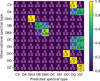 |
Fig. 2 Observed vs predicted (García-Zamora et al. 2025) spectral-type confusion matrix for the 143 white dwarfs assigned a spectral type. Unclassified magnetic white dwarfs as designated as ‘DH’. |
4 General analysis
In this section, we present a general analysis of the spectra of the 255 objects observed with the GTC. We first assessed the capabilities of our random forest algorithm and the correctness of its predictions. Subsequently, we determined the true nature of the ‘massive DB’ subpopulation described in García-Zamora et al. (2025) and Vincent et al. (2024) and its properties. Finally, we analysed the location of our identified objects in the Gaia HR diagram, compared the characteristics of our identified warm and hot DQs with the results of previous studies, and provide first-order estimates of the magnetic fields for selected objects.
4.1 Machine-learning performance
One of the objectives of our observational campaigns was to assess the accuracy of automatic classifications based on machine-learning algorithms. In this subsection, we compare the GTC-based spectral types (hereafter observational spectral types) of 143 objects with those provided in García-Zamora et al. (2025) and Vincent et al. (2024), and derive their classification metrics. We also compare the two automatic classifications against each other.
4.1.1 Comparison with García-Zamora et al. (2025)
We assigned spectroscopic type based on our optical GTC spectra to a total of 143 white dwarfs previously classified by our random forest algorithm as DAH (3), DBs (5), DBAs (8), DOs (6), DQs (25), or DZs (96). We assigned an observational spectral type to 140 of these, while we classified the remaining three objects as strongly magnetic, with no main spectral type assigned. Fig. 2 shows a confusion matrix comparing the predicted and observational classifications. Additionally, we present classification metrics in Table 4.
As can be seen from the nearly diagonal matrix, the results show very good agreement between machine-learning predictions and visually assigned spectroscopic classifications, with 129 objects (90.21%) assigned to the correct spectral type. Our algorithm correctly predicted all observed DAHs, DOs, DQs, and DZs. The main sources of discrepancy are the identification of DC and DA white dwarfs, as well as misclassification at the DB and DBA subtype level. Additionally, we identified two objects as CVs (Section 3.8), a class not included in the training set and therefore impossible to classify correctly.
Classification metrics for the observational sample vs. García-Zamora et al. (2025) comparison.
 |
Fig. 3 Observed vs predicted spectral-type (Vincent et al. 2024) confusion matrix for the 143 white dwarfs assigned a spectral type. Unclassified magnetic white dwarfs as designated as ‘DH’. |
4.1.2 Comparison with Vincent et al. (2024)
We also compared the observational classification of these 143 objects with the automatic classification by Vincent et al. (2024). This classification only considered the DA, DB, DC, DO, DQ, and DZ primary types; no subtypes such as DAH or DBA were considered. Additionally, we assigned objects with uncertain classification (e.g. DA:) to that primary type.
Fig. 3 shows the results. A total of 132 of the 143 objects (92.31% accuracy) are correctly classified. As mentioned above, CVs and magnetic objects could not be correctly classified due to their absence from the training set. All DAs and one DC are correctly classified. However, three DQs and one DZ appear to be misclassified. Table 5 shows the classification metrics for this comparison.
4.1.3 García-Zamora et al. (2025) and Vincent et al. (2024) classifications comparison
At first glance, the classification of Vincent et al. (2024) appears to be slightly more accurate than that of García-Zamora et al. (2025); however, it is important to emphasise that Vincent et al. (2024) does not perform spectral subtype classifications. Thus, if DAHs are grouped with DAs and DBAs with DBs, both works correctly classify 132 of the 143 objects (92.31%). This result demonstrates the robustness of independent machine-learning algorithms.
Classification metrics for the observational sample vs. Vincent et al. (2024) comparison.
Breakdown by spectral type of ‘massive DB’ white dwarfs observed in different spectroscopic campaigns.
4.2 True nature of massive DBs
For the 2024B, 2025A, and 2025B semesters, we selected 170 objects belonging to the ‘massive DB’ sample drawn from the García-Zamora et al. (2025) and Vincent et al. (2024) catalogues for follow-up spectroscopy. Of these, we eventually observed 112 (65.88%) and assigned spectral types to them. This sample is statistically significant enough to derive meaningful conclusions.
Prior to the observational campaigns, we conducted a preliminary search for these objects in the MWDD. We found only a few objects; at most 20% were classified as DB subtypes, while warm DQs and magnetic white dwarfs constitute the majority. However, in our observations, we identify only five DBs (4.46%) among the 112 classified objects. In contrast, we find one DAQ, 23 warm DQs, four hot DQs, and 51 magnetic objects. Of these, 11 are DAHs, four are hot DQHs, and 36 remain unclassified. Table 6 shows a detailed breakdown of these results.
These proportions indicate that, despite its designation, the ‘massive DB’ subpopulation is not composed of genuinely massive DB white dwarfs but rather of a collection of objects with peculiar spectra that are misclassified as DBs. We did not include these very rare spectral types nor the strongly magnetic objects in the training sets, and therefore these classifications were not available for the algorithm. As a result, the algorithm assigned these objects to the closest available category, which happened to be DBs.
4.3 DA analysis
The location of the observed DAs in the HR diagram separates them into two groups (see Fig. A.1 in Appendix A, top-left panel): the massive and the non-massive samples. The non-massive DAs are found along the upper part of the white dwarf locus and are relatively cool objects. Most of the massive DAs are located above the Q-branch, with a few within it and one DAB and one DAH below it.
Additionally, four DAs are massive and very hot (GBP − GRP < −0.36). These four objects may represent the hottest end of the DA→DAQ→DQA evolutionary sequence for warm DQs proposed by Kilic et al. (2024). For further details, we refer to Sect. 4.7.2.
4.4 DB analysis
As shown in the Gaia HR diagram (Appendix A, Fig. A.1, top-right panel), most of the identified DBs occupy a narrow colour range around GBP − GRP ≈ 0. Five of them (three DBs and two DBAs) are massive DB white dwarfs. Although they do not form a statistically meaningful sample, these objects still provide valuable information on massive DB white dwarfs. For instance, if they pulsate, their interiors can be studied through asteroseismology. Pulsating DB white dwarfs are expected to be hotter and considerably less crystallised than pulsating DAs (Córsico et al. 2021), allowing us to probe their deep interiors.
Interestingly, four of the objects have unusually high luminosities and are hence located slightly above the main cooling track. Currently, we have no observations that allow us to determine whether they are low-mass white dwarfs or unresolved binary objects.
4.5 DC analysis
As stated in Sect. 3.3, 24 of the DCs in our sample are hot objects with GBP − GRP < 0.1 (see Fig. A.1, Appendix A, second row, left panel). However, these two facts are contradictory since such high temperatures should be sufficient for these objects to display spectral lines. The most likely explanation is that these objects are highly magnetic, with magnetic field strengths high enough to suppress spectral lines in the optical range (Jewett et al. 2024). However, we did not carry out polarimetric observations during our campaigns that could measure their magnetic fields, and therefore we have no direct measurements of their field strengths.
4.6 DO analysis
We identify two pure DOs and four DOZs. The DOZ objects are a short intermediate phase between pre-degenerate PG 1159 objects and pure DOs, which takes place during the gravitational settling of heavier elements (Bédard et al. 2022a). Therefore, DOZ white dwarfs would be expected to be hotter than pure DOs, which is not what we observe in the Gaia HR diagram (Fig. A.1 in Appendix A, top-right panel). Although six objects do not constitute a statistically significant sample, it is worth noting that Unglaub & Bues (2000) suggest that different initial compositions of PG 1159 objects might cause the PG 1159 to DO transition to occur at different temperatures. By extension, the transitional DOZ phase would also take place at different temperatures, hence colours, for different objects. This difference would explain the observed distribution.
4.7 Carbon-rich stars
Warm and hot DQs are rare and poorly understood objects. In recent years, several studies (e.g. Koester & Kepler 2019; Coutu et al. 2019; Kilic et al. 2024, 2025) have shed light on the properties, parameters, and evolution of these white dwarfs.
In this section, we present an analysis of the different DQ subpopulations identified in this work. This includes both their location in the Gaia HR diagram and their kinematics, as well as a comparison with the results of recent studies such as Coutu et al. (2019) and Kilic et al. (2025).
4.7.1 DQ subpopulations
White dwarfs with carbon features do not constitute a homogeneous subpopulation. Rather, they separate into two distinct subpopulations: on the one hand, the cool, classical DQs; on the other hand, the warm and hot DQs (see, for instance, Dufour et al. 2013; Fortier & Dufour 2015; Coutu et al. 2019; Koester & Kepler 2019).
The distinction between the cool DQ and the warm-hot DQ subpopulations is not based only on their different temperatures but also on their stellar parameters (e.g. mass), atmospheric composition, and proposed origins. Both warm and hot DQs are more massive than classical cool DQs (see e.g. Koester & Kepler 2019; Coutu et al. 2019; Kilic et al. 2025; Ould Rouis et al. 2026). A very high proportion of hot DQs is also magnetic (Dufour et al. 2013); magnetic warm DQs, however, are much rarer (Ould Rouis et al. 2026), Williams et al. (2013) providing an example. Regarding their atmospheres, warm and hot DQs are dominated by carbon (Dufour et al. 2007, 2008), with hydrogen as a trace element (Koester & Kepler 2019; Kilic et al. 2025), while cool DQ atmospheres are helium dominated (Bues 1973), and carbon appears in their spectra as a result of convective dredge-up (Koester et al. 1982; Pelletier et al. 1986). Finally, the kinematics of warm DQs, more specifically their high velocity dispersion, reveal an inconsistency between their cooling and kinematic ages. That is, the cooling ages of warm DQs are small compared to the kinematic ages derived from their motions (Dunlap & Clemens 2015; Coutu et al. 2019; Kawka et al. 2023).
This combination of higher-than-average masses, peculiar atmospheric composition, a high incidence of magnetic fields, and unusual kinematics suggests that a merger-remnant origin may represent one of the most plausible formation channels for warm and hot DQs (Dunlap & Clemens 2015; Coutu et al. 2019; Kawka et al. 2023). Cool DQs, on the other hand, are the result of single-object evolution and are one of the final proposed steps in the evolutionary sequence of helium-rich objects (Bédard et al. (2022b), see also Fig. 13 in Bédard 2024). In the following subsections, we present an analysis of these aspects for the warm and hot DQs in our sample, focusing on whether our results agree with previous studies.
4.7.2 Location in the Gaia HR diagram
Once the DQs are placed in the Gaia HR diagram (Appendix A, Fig. A.1), the two subpopulations occupy markedly different regions. Cool DQs lie along the main cooling track, with GBP − GRP colours greater than ≃0.5 mag. Warm DQs are concentrated on the Q-branch and the crystallisation sequence. Finally, hot DQs at located in the bluer end of the white dwarf locus (GBP − GRP ≤ −0.3) and approximately one magnitude above the Q-branch.
The location of our warm DQs is consistent with those analysed by Kilic et al. 2025 (see the top panel of their Fig. 11, as well as their Fig. 12). That is, warm DQs appear along the Q-branch and crystallisation sequences, while hot DQs have not yet reached it. Our single identified DQZA also lies on the Q-branch; the DAQ we identify also lies there, but at a bluer location.
Lastly, we highlight the warm DQs J0517+2633, J0540+3205, J1902+2607, J2024–0234, J2046+3830, and J2323–0623, since, in addition to CI spectral lines, they also display shallow Swan bands centred around λλλ = 4370, 4700, 5100 Å (an example spectrum is shown in Appendix B, Fig. B.3). These objects, located at the cooler end of the Q-branch and displaying warm and cool DQ characteristics, fall under the warm DQ classification according to the definition in Koester & Kepler (2019).
Kilic et al. (2024) propose two evolutionary channels for warm and hot DQs. In the first, DA→DAQ→warm DQA, a thin hydrogen atmosphere is progressively diluted by the carbon-rich envelope as the white dwarf cools. In the second, hot DQ(A)→warm DQ(A), a hot DQ progressively cools into a warm DQ. We suggest that the six objects described in the previous paragraph may provide examples of the final stages of these evolutionary channels.
4.7.3 Magnetic incidence in warm and hot DQs
A very high proportion of hot DQs is reported as magnetic. For instance, Dufour et al. (2013) found ten magnetic objects in a sample of 14 hot DQs (71.43%). By contrast, magnetic fields in warm DQs are rarer, with only a few known examples. Different processes, such as white dwarf-subgiant mergers or magnetic field dissipation, have been invoked as possible explanations (Ould Rouis et al. 2026).
In our classification, we find that all four hot DQs (100%) harbour magnetic fields. However, their intensities vary. For instance, the splitting in J0034+7130 is of only a few Å, J0420+6450 shows a wavelength difference between the split components of a few tens of Å, while band-like structures appear in the spectra of J0446+7227 and J0642+0632. We present an estimate of the magnetic field of J0420+6450 in Sect. 4.9.3.
In contrast to this result, no magnetic warm DQs are found among our 29 identifications. The incidence of magnetism in hot and warm DQs, therefore, is consistent with previous results.
4.7.4 Kinematics of the DQ population
Recent studies suggest that the warm and hot DQ subpopulations display unusual kinematics. For instance, Dunlap & Clemens (2015) and Kilic et al. (2025) report inconsistencies between their kinematic ages and cooling ages, with the former being much greater than the latter. A high proportion of the warm DQ population displays unusually high tangential velocities (vtan ≥ 50 km s−1, used in Wegg & Phinney (2012) as a kinematic ‘smoking gun’ signature of a merger origin for high-mass white dwarfs). Coutu et al. (2019) finds that ten of the 22 warm DQs (45.5%) in their sample show vtan ≥ 50 km s−1. Kilic et al. (2025) report 41 out of 75 warm DQs (54.7%) above this value.
We obtained the tangential velocities of all white dwarfs in our observational campaigns and show them in a colour–vtan diagram (Fig. 4), following Fig. 13 of Kilic et al. 2025. We find that 52 of the 321 objects in our complete observational sample have vtan ≥ 50 km s−1. Of these, 13 are warm DQs. We find a total of 33 warm and hot DQs, of which 11 are pure DQs, 16 are DQAs, one is a DQZA, one is a DAQ, and four are hot DQs. Of these, 39.4% of our warm DQ sample has vtan ≥ 50 km s−1. Although the proportion of warm DQs with unusual kinematics is not as high as that found in Coutu et al. (2019) or Kilic et al. (2025), it is nevertheless unusually high.
For cool DQs, only three out of 15 (20%), two of which are DQpecs, show vtan ≥ 50 km s−1, a fraction close to that found for the whole sample (52 out of 321 objects, 16.20%). The kinematics of cool DQs is therefore compatible with single-object evolution.
 |
Fig. 4 Colour-tangential velocity diagram for our warm DQs. Thirteen of these warm DQs are above the vtan ≥ 50 km s−1 limit. |
4.8 DZ analysis
We display the 90 identified DZs in the Gaia HR diagram in Appendix A, Fig. A.1, third row, right panel. They are mainly found along the B branch. As discussed above, we identify the Ca II H and K lines in all objects, while other metals such as Mg, Fe, or Na are less frequent.
Ten of our objects display weak hydrogen signatures as well as metallic lines. This hydrogen is though to have been accreted from water-rich bodies (Jura & Xu 2012; Gentile Fusillo et al. 2017).
The DZ white dwarfs with helium features are extremely rare objects, with only four cases (two DZAB, one DZBAH, and one DZO) listed in the MWDD. In our campaigns, we identify three more such objects, namely two DZBAs (J0437+0051 and J0745+5551) and one DZAB (J0452–0214), therefore increasing the amount of known objects by 75%. When represented in the Gaia HR diagram (third row, right panel of Fig. A.1 in Appendix A), these objects are hot (GBP − GRP ~ 0), as expected from the presence of He I lines.
4.9 Magnetic object analysis
In addition to the spectroscopically confirmed magnetic white dwarfs discussed above, our sample contains a number of objects displaying clear magnetic signatures. Of the unclassified magnetic objects, 36 are hot and massive, whereas three are cooler and lie along the main cooling track. When represented in the Gaia HR diagram, these objects are located mostly above, albeit close to, the hotter end of the Q-branch, with only a minority lying directly on it. This behaviour is consistent with the location of magnetic white dwarfs reported in the MWDD. However, in the absence of polarimetric observations and without a reliable spectral classification, we cannot determine the magnetic field strengths of these objects from spectroscopy alone.
The Gaia location of these objects in the Gaia HR diagram is shown in the bottom-left panel of Fig. A.1 in Appendix A, while the bottom-right panel shows a zoom of the Q-branch region, highlighting the DAHs, hot DQHs, and massive unclassified magnetic objects.
In the following subsections we estimate the magnetic field strengths of the DAHs, DZHs, and hot DQHs in our sample.
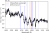 |
Fig. 5 Zeeman splitting of Hβ in DAH J1927+6938, with seven resolved components. |
4.9.1 Magnetic field estimates for DAHs
Based on the magnitude of the Zeeman splitting, we find two different cases, corresponding to different magnetic-field strengths. Three objects display three components in the split Hβ line, whereas the 11 remaining ones show seven. Additionally, the Zeeman splitting of Hα is larger for these objects. This indicates a stronger magnetic field. Fig. 5 shows an example of the seven-component splitting of the Hβ line.
We also performed a first-order estimate of the magnetic field strengths by fitting Gaussian profiles to the visible components of the Hα and Hβ lines. We took the line centre as the mean of the Gaussian fits, and computed the spectral displacement as the wavelength difference between the lateral and central peaks for both components.
Having calculated the spectral displacements, we used Eq. (1) of Reid et al. (2001) to obtain a magnetic-field estimate for each displacement and then averaged them to obtain a final magnetic field for each spectral line. We then obtained the final magnetic field of the white dwarf by averaging the fields inferred from Hα and Hβ. In cases where the Hβ line is further divided into seven components rather than three, we only used the three components of the Hα line for magnetic field estimation.
We present the magnetic fields for each line, as well as the final magnetic field for each of the white dwarfs in Table 7. As expected, the white dwarfs with larger Zeeman splitting have stronger magnetic fields, of the order of 20 MG, whereas objects with narrower splitting have magnetic fields of the order of 10 MG.
Finally, it should be noted that all of our identified DAHs are hot objects (GBP − GRP ≤ 0.02). This contrasts with the distribution of known DAH objects registered in the MWDD, which span a wide range of temperatures, from the hot to the cool end of the white dwarf locus. This result is due to our own selection bias, as we mostly observed hot (GBP − GRP ≤ 0) objects, which precluded us from observing cooler DAHs.
Magnetic field estimations for spectroscopically confirmed DAH white dwarfs.
Magnetic field strengths of identified DZH white dwarfs.
4.9.2 Magnetic field estimates for DZHs
Following the approach we adopted for the magnetic splitting of the Balmer lines in the previous section, we estimated the magnetic field strengths of this subsample using the splitting of the Na I doublet by fitting the three peaks to Gaussian profiles and using Eq. (1) in Reid et al. (2001). Our estimates indicate four objects with magnetic fields of a few MG. Table 8 lists the results.
It is important to note that, in the cases of J0829–0818 and J1543–0247, we were unable to estimate their magnetic fields. For J1543–0247, the low S/N of the spectra prevents a fit to the split components. For J0829–0818, the large number of split components prevents a reliable identification of the lines that belong to each element. However, due to the similarity of this spectrum to that described in Hollands et al. (2023), which corresponded to a DZH with a magnetic field of approximately 30 MG, we suggest that the magnetic field of this object may be of the same order. This would make J0829–0818 one of the DZs with the most intense magnetic fields registered.
4.9.3 Magnetic field estimates for hot DQHs
All four identified hot DQHs are, as expected, very hot objects with colour GBP − GRP < −0.32, and are located about one magnitude above the Q-branch. We attempted to estimate the magnetic field strengths of the identified DQHs. However, this was only possible for J0420+6450, for which the field was derived by fitting the split components of the C II λλ = 6579, 6582 Å doublet. As in the case of the Na I doublet described in Sect. 4.9.2, this C II doublet becomes a triplet in the presence of a strong magnetic field. The resulting estimate for this object is B = 1.87 ± 0.11 MG.
In the case of J0034+7130, the Zeeman splitting is too weak to reliably identify this split triplet. However, judging by its similarity to the spectra shown in Fig. 2 of Dufour et al. (2013), which have magnetic fields of a few hundred kG, we conclude that this object likely harbours a magnetic field weaker than 1 MG.
Finally, the band structure of the spectra of J0446+7227 and J0642+0632 also prevents the correct identification of the split components. Their fields, however, must be stronger than that of J0420+6450.
5 Conclusions and future perspectives
In this work, we obtain medium-resolution optical spectra of 255 white dwarfs with GTC over four observing campaigns. We investigated the reliability of machine-learning-based spectral classifications derived from Gaia data, by comparing visual classifications from the GTC spectra with those predicted by García-Zamora et al. (2023); García-Zamora et al. (2025). We also clarified the nature of specific subpopulations identified by these methods, in particular the so-called massive (M ≥ 0.95 M⊙) DB white dwarfs.
This analysis enables both a direct validation of automated classifications through comparison with spectroscopic observations and a detailed characterisation of the underlying white dwarf population. Our main contributions can be summarised as follows.
We present a quantitative evaluation of the performance of machine-learning algorithms for spectral classification within a large Gaia-selected sample of white dwarfs. This allows a direct comparison between automated classifications based on Gaia data and those obtained by medium-resolution spectroscopy.
We provide a definitive characterisation of the so-called ‘massive DB’ population, showing that only ~4.5% of these objects are genuine DB white dwarfs, while the majority are magnetic white dwarfs or warm and hot DQs, thus providing the first systematic spectroscopic confirmation of their true nature.
We present an observational characterisation of warm and hot DQ white dwarfs, including their location in the Gaia HR diagram and their kinematic properties, which are consistent with previous works (Coutu et al. 2019; Kilic et al. 2024, 2025) and support a merger-origin scenario.
We identify a significant population of magnetic white dwarfs (63 objects), many of them massive and located near the Q-branch, contributing to our understanding of the incidence of magnetism in this region.
A more detailed breakdown of the results is given below:
We identify a total of 26 DAs, 18 DBs, 27 DCs, six DOs, 47 DQs, 90 DZs, two CVs, and 39 unclassified magnetic objects.
We confirm the high precision of the random forest algorithm described in García-Zamora et al. (2023) and García-Zamora et al. (2025) for spectral type classification. Only 14 objects (9.79%) deviate from the predicted spectral type, five of which belong to types not included in the training set;
Only five of the 112 ‘massive DB’ white dwarfs (MWD ≥ 0.95 M⊙) pre-classified by machine learning algorithms are true DBs. Of these, three (J0622+6935, J0903–1311, and J1832+0856) are pure DBs and two (J0737+5728 and J0847+3222) are DBAs. We assigned spectral types to the remaining 107 objects, classifying them as DAs, DAHs, DCs, or warm and hot DQ(A)s, or unclassified magnetic.
We detect secondary spectral characteristics in 63 of the GTC spectra that were undetected in the low-resolution Gaia spectra, allowing a more precise subclassification of these objects. These objects belong to rare and extremely rare spectral types including two DABs, 14 DAHs, one DAQ, 8 DBAs, one DBAZ, four DOZs, 16 warm DQAs, one DQZA, seven DZAs, one DZAB, two DZBAs, and six DZHs;
The identified subspectral characteristics increase the number of such known objects in the MWDD by two DABs (1.82%), nine DAHs (1.37%), seven DBAs (1.51%), one DBAZ (2.6%), four DOZs (10.25%), 12 warm DQAs (16.22%), one DQZA (50%), seven DZAs (7.45%), one DZAB (50%), two DZBAs (200%), and four DZHs (20%);
We find 24 massive (MWD ≥ 0.95 M⊙) and hot (0.10 ≥ GBP − GRP) DCs, which are expected to be highly magnetic;
Excluding the 24 DCs, we identify 63 newly identified magnetic objects. Of these, 14 are DAHs, six are DZHs, four are hot DQHs, and 39 remain unclassified due to their spectral features not matching any known spectral lines. Of these 63 objects, 51 (11 DAHs, four hot DQHs, and 36 unclassified) are massive (M ≥ 0.95 M⊙). These 51 objects, together with the 24 massive DCs identified above, will help to improve our understanding of the origin and incidence of magnetic fields in massive white dwarfs;
We confirm 14 new magnetic DAHs objects, 11 of which are massive (MWD ≥ 0.95 M⊙). From the field estimate described in Sect. 4.9.1, three DAHs have magnetic fields of the order of 10 MG; while the remaining 11 have fields of the order of 20 MG;
We identify six new magnetic DZH white dwarfs. First-order estimates for their magnetic fields (see Sect. 4.9.2) place them in the 1–4 MG range;
We identify four new magnetic hot DQHs (J0034+7130, J0420+6450, J0446+7227 and J0642+0632) with different field strengths. The magnetic field of J0420+6450 is estimated to be of the order of 2 MG.
We identify two new CVs (J2007+1742 and J2250+6328).
For the warm and hot DQs, our main findings can be summarised as follows:
We identify a total of 29 warm DQs and four hot DQs have been identified;
Of the 29 warm DQs, 11 are pure DQs, 16 are DQAs, one is a DQZA (J0328+5806), and one is a DAQ (J0325+2540);
Of the warm DQs, six of them show weak Swan bands in addition to CI lines. These objects may provide examples of the evolutionary pipelines for warm DQs described in Kilic et al. (2024);
The location of our 29 warm DQs in the Gaia HR diagram agrees with the findings of Kilic et al. (2025) as they are located in the Q-branch and the CO-core crystallisation sequence.
Our four hot DQs are located approximately one magnitude above the Q-branch;
The magnetic fraction for hot and warm DQs is consistent with previously published results;
We find that 13 of our 33 (39.4%) warm and hot DQs exhibit unusually high tangential velocities (vtan ≥ 50 km s−1). Our kinematics results are consistent with those reported by Coutu et al. (2019) and Kilic et al. (2025);
Our only identified DAQ (J0325+2540) is located on the Q-branch and shows a very high (vtan ≥ 140 km s−1) tangential velocity. This is consistent with previously reported DAQs and supports the idea that DAQs and warm DQs differ only in their atmospheric carbon abundances (Kilic et al. 2024).
Future perspectives on this work are twofold:
Although we have obtained new insights into massive magnetic objects, as well as warm and hot DQs, further information is still required regarding their connection with the rest of the Q-branch population. To address this, new spectroscopical campaigns have been proposed targeting Q-branch objects without prior spectral type distinction. These data will be complemented by future data releases from the DESI (Levi et al. 2019), 4MOST (de Jong et al. 2019), and WEAVE (Jin et al. 2024) surveys;
Despite some magnetic ‘massive DBs’ being identified as DAH and hot DQH white dwarfs, 36 out of 51 (70.59%) still lack a reliable spectral type. Polarimetric observations to determine their magnetic field intensity would be valuable for constraining their nature.
Data availability
The data underlying this article are available in the article. Supplementary material will be shared on reasonable request to the corresponding author. Table 3 is available at the CDS via https://cdsarc.cds.unistra.fr/viz-bin/cat/J/A+A/711/A70.
Acknowledgements
We acknowledge support from MINECO under the PID2023-148661NB-I00 grant and by the AGAUR/Generalitat de Catalunya grant SGR-386/2021. Enrique Miguel García Zamora also acknowledges financial support from Banco de Santander, under a Becas Santander Investigación/Ajuts de Formació de Professorat Universitari (2022_FPU-UPC_16) grant. Based on observations made with the Gran Telescopio Canarias (programmes GTC20-23B, GTC28-24B, GTC36-25A, GTC8-25B), installed in the Spanish Observatorio del Roque de los Muchachos of the Instituto de Astrofísica de Canarias, in the island of La Palma.
References
- Althaus, L. G., Córsico, A. H., Isern, J., & García-Berro, E. 2010, A&A Rev., 18, 471 [NASA ADS] [CrossRef] [Google Scholar]
- Bédard, A. 2024, Ap&SS, 369, 43 [CrossRef] [Google Scholar]
- Bédard, A., Bergeron, P., & Brassard, P. 2022a, ApJ, 930, 8 [Google Scholar]
- Bédard, A., Brassard, P., Bergeron, P., & Blouin, S. 2022b, ApJ, 927, 128 [Google Scholar]
- Bergeron, P., Wesemael, F., Dufour, P., et al. 2011, ApJ, 737, 28 [Google Scholar]
- Bergeron, P., Dufour, P., Fontaine, G., et al. 2019, ApJ, 876, 67 [NASA ADS] [CrossRef] [Google Scholar]
- Blouin, S., Dufour, P., Thibeault, C., & Allard, N. F. 2019, ApJ, 878, 63 [NASA ADS] [CrossRef] [Google Scholar]
- Blouin, S., Bédard, A., & Tremblay, P.-E. 2023, MNRAS, 523, 3363 [NASA ADS] [CrossRef] [Google Scholar]
- Bues, I. 1973, A&A, 28, 181 [Google Scholar]
- Camisassa, M. E., Althaus, L. G., Córsico, A. H., et al. 2019, A&A, 625, A87 [NASA ADS] [CrossRef] [EDP Sciences] [Google Scholar]
- Camisassa, M., Torres, S., Hollands, M., et al. 2023, A&A, 674, A213 [NASA ADS] [CrossRef] [EDP Sciences] [Google Scholar]
- Camisassa, M., Baiko, D. A., Torres, S., & Rebassa-Mansergas, A. 2024, A&A, 683, A101 [NASA ADS] [CrossRef] [EDP Sciences] [Google Scholar]
- Carrasco, J. M., Weiler, M., Jordi, C., et al. 2021, A&A, 652, A86 [NASA ADS] [CrossRef] [EDP Sciences] [Google Scholar]
- Cepa, J., Bongiovanni, A., Pérez García, A. M., et al. 2013, in Highlights of Spanish Astrophysics VII, eds. J. C. Guirado, L. M. Lara, V. Quilis, & J. Gorgas, 868 [Google Scholar]
- Córsico, A. H., Althaus, L. G., Gil-Pons, P., & Torres, S. 2021, A&A, 646, A60 [NASA ADS] [CrossRef] [EDP Sciences] [Google Scholar]
- Coutu, S., Dufour, P., Bergeron, P., et al. 2019, ApJ, 885, 74 [NASA ADS] [CrossRef] [Google Scholar]
- Cunningham, T., Tremblay, P.-E., Gentile Fusillo, N. P., Hollands, M., & Cukanovaite, E. 2020, MNRAS, 492, 3540 [NASA ADS] [CrossRef] [Google Scholar]
- De Angeli, F., Weiler, M., Montegriffo, P., et al. 2023, A&A, 674, A2 [NASA ADS] [CrossRef] [EDP Sciences] [Google Scholar]
- de Jong, R. S., Agertz, O., Berbel, A. A., et al. 2019, The Messenger, 175, 3 [NASA ADS] [Google Scholar]
- Dufour, P., Liebert, J., Fontaine, G., & Behara, N. 2007, Nature, 450, 522 [Google Scholar]
- Dufour, P., Fontaine, G., Liebert, J., Schmidt, G. D., & Behara, N. 2008, ApJ, 683, 978 [Google Scholar]
- Dufour, P., Blouin, S., Coutu, S., et al. 2017, in Astronomical Society of the Pacific Conference Series, 509, 20th European White Dwarf Workshop, eds. P. E. Tremblay, B. Gaensicke, & T. Marsh, 3 [Google Scholar]
- Dufour, P., Vornanen, T., Bergeron, P., & Fontaine, A. B., 2013, in Astronomical Society of the Pacific Conference Series, 469, 18th European White Dwarf Workshop., eds. J. Krzesiński, G. Stachowski, P. Moskalik, & K. Bajan, 167 [Google Scholar]
- Dunlap, B. H., & Clemens, J. C. 2015, in Astronomical Society of the Pacific Conference Series, 493, 19th European Workshop on White Dwarfs, eds. P. Dufour, P. Bergeron, & G. Fontaine, 547 [Google Scholar]
- Farihi, J., Barstow, M. A., Redfield, S., Dufour, P., & Hambly, N. C. 2010, MNRAS, 404, 2123 [NASA ADS] [Google Scholar]
- Fortier, A., & Dufour, P. 2015, in Astronomical Society of the Pacific Conference Series, 493, 19th European Workshop on White Dwarfs, eds. P. Dufour, P. Bergeron, & G. Fontaine, 41 [Google Scholar]
- Gaia Collaboration (Prusti, T., et al.) 2016, A&A, 595, A1 [NASA ADS] [CrossRef] [EDP Sciences] [Google Scholar]
- Gänsicke, B. T., Koester, D., Girven, J., Marsh, T. R., & Steeghs, D. 2010, Science, 327, 188 [Google Scholar]
- García-Zamora, E. M., Torres, S., & Rebassa-Mansergas, A. 2023, A&A, 679, A127 [NASA ADS] [CrossRef] [EDP Sciences] [Google Scholar]
- García-Zamora, E. M., Torres, S., Rebassa-Mansergas, A., & Ferrer-Burjachs, A. 2025, A&A, 699, A3 [NASA ADS] [CrossRef] [EDP Sciences] [Google Scholar]
- Genest-Beaulieu, C., & Bergeron, P. 2019, ApJ, 871, 169 [NASA ADS] [CrossRef] [Google Scholar]
- Gentile Fusillo, N. P., Gänsicke, B. T., Farihi, J., et al. 2017, MNRAS, 468, 971 [NASA ADS] [CrossRef] [Google Scholar]
- Hall, P. B., & Maxwell, A. J. 2008, ApJ, 678, 1292 [Google Scholar]
- Hollands, M. A., Tremblay, P. E., Gänsicke, B. T., Gentile-Fusillo, N. P., & Toonen, S. 2018, MNRAS, 480, 3942 [NASA ADS] [CrossRef] [Google Scholar]
- Hollands, M. A., Tremblay, P.-E., Gänsicke, B. T., et al. 2020, Nat. Astron., 4, 663 [CrossRef] [Google Scholar]
- Hollands, M. A., Stopkowicz, S., Kitsaras, M.-P., et al. 2023, MNRAS, 520, 3560 [NASA ADS] [CrossRef] [Google Scholar]
- Jewett, G., Kilic, M., Bergeron, P., et al. 2024, ApJ, 974, 12 [Google Scholar]
- Jiménez-Esteban, F. M., Torres, S., Rebassa-Mansergas, A., et al. 2023, MNRAS, 518, 5106 [Google Scholar]
- Jin, S., Trager, S. C., Dalton, G. B., et al. 2024, MNRAS, 530, 2688 [NASA ADS] [CrossRef] [Google Scholar]
- Jura, M., & Xu, S. 2012, AJ, 143, 6 [NASA ADS] [CrossRef] [Google Scholar]
- Kawka, A., Ferrario, L., & Vennes, S. 2023, MNRAS, 520, 6299 [NASA ADS] [CrossRef] [Google Scholar]
- Kepler, S. O., Pelisoli, I., Koester, D., et al. 2015, MNRAS, 446, 4078 [Google Scholar]
- Kilic, M., Bergeron, P., Blouin, S., et al. 2024, ApJ, 965, 159 [Google Scholar]
- Kilic, M., Bergeron, P., Brown, W. R., et al. 2025, ApJ, 990, 62 [Google Scholar]
- Kilic, M., Bergeron, P., Moss, A., et al. 2026, arXiv e-prints [arXiv:2602.07246] [Google Scholar]
- Koester, D., & Kepler, S. O. 2019, A&A, 628, A102 [NASA ADS] [CrossRef] [EDP Sciences] [Google Scholar]
- Koester, D., Weidemann, V., & Zeidler, E.-M. 1982, A&A, 116, 147 [NASA ADS] [Google Scholar]
- Levi, M., Allen, L. E., Raichoor, A., et al. 2019, in Bulletin of the American Astronomical Society, 51, 57 [Google Scholar]
- Liebert, J., Harris, H. C., Dahn, C. C., et al. 2003, AJ, 126, 2521 [Google Scholar]
- Marsh, T. R. 2014, PAMELA: Optimal extraction code for long-slit CCD spectroscopy, Astrophysics Source Code Library [record ascl:1406.002] [Google Scholar]
- Marsh, T. 2019, molly: 1D astronomical spectra analyzer, Astrophysics Source Code Library [record ascl:1907.012] [Google Scholar]
- O’Brien, M. W., Tremblay, P. E., Gentile Fusillo, N. P., et al. 2023, MNRAS, 518, 3055 [Google Scholar]
- Ould Rouis, L. B., Hermes, J. J., Guidry, J. A., et al. 2026, arXiv e-prints [arXiv:2602.02670] [Google Scholar]
- Pelletier, C., Fontaine, G., Wesemael, F., Michaud, G., & Wegner, G. 1986, ApJ, 307, 242 [NASA ADS] [CrossRef] [Google Scholar]
- Pérez-Couto, X., Pallas-Quintela, L., Manteiga, M., Villaver, E., & Dafonte, C. 2024, ApJ, 977, 31 [Google Scholar]
- Reid, I. N., Liebert, J., & Schmidt, G. D. 2001, ApJ, 550, L61 [Google Scholar]
- Sion, E. M., Greenstein, J. L., Landstreet, J. D., et al. 1983, ApJ, 269, 253 [CrossRef] [Google Scholar]
- Tremblay, P. E., Cukanovaite, E., Gentile Fusillo, N. P., Cunningham, T., & Hollands, M. A. 2019a, MNRAS, 482, 5222 [Google Scholar]
- Tremblay, P.-E., Fontaine, G., Gentile Fusillo, N. P., et al. 2019b, Nature, 565, 202 [Google Scholar]
- Unglaub, K., & Bues, I. 2000, A&A, 359, 1042 [NASA ADS] [Google Scholar]
- Vincent, O., Bergeron, P., & Dufour, P. 2023, MNRAS, 521, 760 [NASA ADS] [CrossRef] [Google Scholar]
- Vincent, O., Barstow, M. A., Jordan, S., et al. 2024, A&A, 682, A5 [NASA ADS] [CrossRef] [EDP Sciences] [Google Scholar]
- Warner, B. 1995, Cataclysmic Variable Stars, 28 [Google Scholar]
- Wegg, C., & Phinney, E. S. 2012, MNRAS, 426, 427 [NASA ADS] [CrossRef] [Google Scholar]
- Williams, R. E. 1980, ApJ, 235, 939 [Google Scholar]
- Williams, G. 1983, ApJS, 53, 523 [NASA ADS] [CrossRef] [Google Scholar]
- Williams, K. A., Winget, D. E., Montgomery, M. H., et al. 2013, ApJ, 769, 123 [NASA ADS] [CrossRef] [Google Scholar]
- Zuckerman, B., Koester, D., Melis, C., Hansen, B. M., & Jura, M. 2007, ApJ, 671, 872 [Google Scholar]
Appendix A Gaia colour-magnitude diagrams for the visually identified spectral types and subtypes
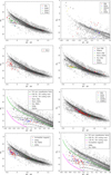 |
Fig. A.1 Gaia HR diagram for the identified DAs (first row, left panel), DBs and DOs (first row, right panel), DCs (second row, left panel), DQs (second row, right; and third row, left panels), DZs (third row, right panel) and magnetic objects (fourth row, both panels). |
Appendix B Sample spectra of selected objects
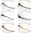 |
Fig. B.1 GTC spectra of a pure DA (first panel), a DAB (second panel), a DAH (third panel), a DAQ (fourth panel), a pure DB (fifth panel) and a DBA (sixth panel). |
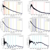 |
Fig. B.2 GTC spectra of a DBAZ (first panel), a DC (second panel), a pure DO (third panel), a DOZ (fourth panel), a cool DQ (fifth panel) and a DQpec (sixth panel). |
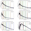 |
Fig. B.3 GTC spectra of a warm DQ (first panel), a warm DQA (second panel), a warm DQ displaying both weak C2 Swan bands and C I spectral lines (third panel), a hot DQ (fourth panel), a warm DQZA (fifth panel) and a pure DZ (sixth panel). |
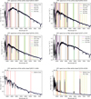 |
Fig. B.4 GTC spectra of a DZA (first panel), a DZAB (second panel), a DZBZ (third panel), a DZH (fourth panel), an unclassified magnetic white dwarf with clear signs of Zeeman splitting (fifth panel) and a CV (sixth panel). |
Developed by Tom Marsh and available at https://cygnus.astro.warwick.ac.uk/phsaap/software/molly/html/INDEX.html
All Tables
Classification metrics for the observational sample vs. García-Zamora et al. (2025) comparison.
Classification metrics for the observational sample vs. Vincent et al. (2024) comparison.
Breakdown by spectral type of ‘massive DB’ white dwarfs observed in different spectroscopic campaigns.
All Figures
|
Fig. 1 Gaia HR diagram of the targets observed at the GTC during the 2023B, 2024B, 2025A, and 2025B semesters, superimposed on the Gaia 100 pc white dwarf sample of Jiménez-Esteban et al. (2023). |
| In the text | |
|
Fig. 2 Observed vs predicted (García-Zamora et al. 2025) spectral-type confusion matrix for the 143 white dwarfs assigned a spectral type. Unclassified magnetic white dwarfs as designated as ‘DH’. |
| In the text | |
|
Fig. 3 Observed vs predicted spectral-type (Vincent et al. 2024) confusion matrix for the 143 white dwarfs assigned a spectral type. Unclassified magnetic white dwarfs as designated as ‘DH’. |
| In the text | |
|
Fig. 4 Colour-tangential velocity diagram for our warm DQs. Thirteen of these warm DQs are above the vtan ≥ 50 km s−1 limit. |
| In the text | |
|
Fig. 5 Zeeman splitting of Hβ in DAH J1927+6938, with seven resolved components. |
| In the text | |
|
Fig. A.1 Gaia HR diagram for the identified DAs (first row, left panel), DBs and DOs (first row, right panel), DCs (second row, left panel), DQs (second row, right; and third row, left panels), DZs (third row, right panel) and magnetic objects (fourth row, both panels). |
| In the text | |
|
Fig. B.1 GTC spectra of a pure DA (first panel), a DAB (second panel), a DAH (third panel), a DAQ (fourth panel), a pure DB (fifth panel) and a DBA (sixth panel). |
| In the text | |
|
Fig. B.2 GTC spectra of a DBAZ (first panel), a DC (second panel), a pure DO (third panel), a DOZ (fourth panel), a cool DQ (fifth panel) and a DQpec (sixth panel). |
| In the text | |
|
Fig. B.3 GTC spectra of a warm DQ (first panel), a warm DQA (second panel), a warm DQ displaying both weak C2 Swan bands and C I spectral lines (third panel), a hot DQ (fourth panel), a warm DQZA (fifth panel) and a pure DZ (sixth panel). |
| In the text | |
|
Fig. B.4 GTC spectra of a DZA (first panel), a DZAB (second panel), a DZBZ (third panel), a DZH (fourth panel), an unclassified magnetic white dwarf with clear signs of Zeeman splitting (fifth panel) and a CV (sixth panel). |
| In the text | |
Current usage metrics show cumulative count of Article Views (full-text article views including HTML views, PDF and ePub downloads, according to the available data) and Abstracts Views on Vision4Press platform.
Data correspond to usage on the plateform after 2015. The current usage metrics is available 48-96 hours after online publication and is updated daily on week days.
Initial download of the metrics may take a while.