


| Issue |
A&A
Volume 711, July 2026
|
|
|---|---|---|
| Article Number | A186 | |
| Number of page(s) | 15 | |
| Section | Cosmology (including clusters of galaxies) | |
| DOI | https://doi.org/10.1051/0004-6361/202659262 | |
| Published online | 16 July 2026 | |
Predicting galaxy bias using machine learning
1
Departamento de Física, Universidad Técnica Federico Santa María, Av. España 1680, Valparaíso, Chile
2
HEP Division, Argonne National Laboratory, 9700 South Cass Avenue, Lemont, IL, 60439, USA
3
Berkeley Center for Cosmological Physics, University of California, Berkeley, 341 Campbell Hall, Berkeley, CA, 94720, U.S.A.
4
Physics Division, Lawrence Berkeley National Laboratory, 1 Cyclotron Road, Berkeley, CA, 94720, U.S.A.
5
Departamento de Física Matemática, Instituto de Física, Universidade de São Paulo, Rua do Matão 1371, CEP 05508-090, São Paulo, Brazil
6
Universidad Andres Bello, Facultad de Ciencias Exactas, Departamento de Fisica y Astronomia, Instituto de Astrofisica, Fernandez Concha 700, Las Condes, Santiago RM, Chile
7
Independent Researcher., Camino El Pino 68D, 38208, La Laguna, Spain
★ Corresponding authors: This email address is being protected from spambots. You need JavaScript enabled to view it.
; This email address is being protected from spambots. You need JavaScript enabled to view it.
Received:
2
February
2026
Accepted:
4
May
2026
Abstract
Context. Understanding how galaxies trace the underlying matter density field is essential for characterizing the influence of the large-scale structure on galaxy formation, being therefore a key ingredient in observational cosmology. This connection, commonly described through the galaxy bias, b, can be studied effectively using machine-learning (ML) techniques, which offer strong predictive capabilities and can capture nonlinear relationships in high-dimensional data. Recent work has also highlighted the need for probabilistic methods to properly account for the intrinsic stochasticity of this connection.
Aims. We aim to incorporate the linear bias parameter assigned to individual galaxies into a ML framework, quantify its dependence on various halo and environmental properties, and evaluate whether different algorithms can accurately predict this parameter and reproduce the scatter in several bias relations.
Methods. We use data from the IllustrisTNG300 magnetohydrodynamical simulation, including the distance to different cosmic web structures computed with DisPerSE. These data are complemented with an object-by-object estimator of the large-scale linear bias (bi), providing the individual contribution of each galaxy to the bias of the entire population. Our ML framework uses three models to predict bi: a random forest regressor, a single-output neural network and a probabilistic method (normalizing flows).
Results. We recover the full hierarchy of galaxy bias dependencies, showing that the most informative features are the overdensities, particularly δ8, followed by the distances to cosmic-web structures and selected internal halo properties, most notably the formation redshift (z1/2). We also demonstrate that normalizing flows clearly outperform deterministic methods in predicting galaxy bias, including its joint distributions with galaxy properties, owing to their ability to capture the intrinsic variance associated with the stochastic nature of the matter-halo-galaxy connection. Our ML framework provides a foundation for future efforts to measure the individual bias with upcoming spectroscopic surveys.
Key words: galaxies: evolution / galaxies: formation / galaxies: halos / galaxies: statistics / dark matter / large-scale structure of Universe
© The Authors 2026
 Open Access article, published by EDP Sciences, under the terms of the Creative Commons Attribution License (https://creativecommons.org/licenses/by/4.0), which permits unrestricted use, distribution, and reproduction in any medium, provided the original work is properly cited.
This article is published in open access under the Subscribe to Open model. This email address is being protected from spambots. You need JavaScript enabled to view it. to support open access publication.
1. Introduction
From a cosmological perspective, it is often useful to view the Universe as composed of three interconnected layers: the continuous matter density field, the discrete field of dark matter (DM) halos, and the discrete field of galaxies, which form through the cooling and condensation of gas within the halos’ potential wells (White & Rees 1978). Characterizing the mapping between these cosmic fields has key implications for models of galaxy formation and for the extraction of cosmological information from galaxy surveys, motivating the ongoing development of innovative analytical, computational, and theoretical techniques (Wechsler & Tinker 2018).
In this context, machine learning (ML) has emerged as a powerful approach for capturing nonlinear relationships in high-dimensional data, improving the efficiency and accuracy of simulations, emulators, and cosmological inference as a whole (e.g., Lucie-Smith et al. 2018; Peel et al. 2019; Villaescusa-Navarro et al. 2021; Kreisch et al. 2022; Perez et al. 2024). ML has also become an integral part of the standard toolkit for exploring the halo-galaxy connection, not only for its ability to reproduce the complex relationships between galaxies and DM halos, but also for its potential to shed light on the physical mechanisms underlying this fundamental link (Jo & Kim 2019; Stiskalek et al. 2022; de Santi et al. 2022; Jespersen et al. 2022; Rodrigues et al. 2023; Lovell et al. 2023; Sullivan et al. 2023; Chuang et al. 2024; Rodrigues et al. 2025). Importantly, recent studies have emphasized the need for a probabilistic framework to predict galaxy properties based on halo and environmental properties, reflecting the inherent stochasticity of the underlying physical processes (Rodrigues et al. 2023; Balaguera-Antolínez et al. 2023; Rodrigues et al. 2025).
The bias of halos and galaxies – relating their overdensities and clustering to those of the underlying matter density field – provides an analytical bridge between the aforementioned cosmic fields (e.g., Kaiser 1984; Efstathiou et al. 1988; Mo & White 1996; Desjacques et al. 2018). In this framework, linear halo bias is often defined as the ratio of power spectra (or correlation functions), b = Phm(k)/Pmm(k)1, which on large scales recovers the expectation from peak–background split theory for a given population of objects (see e.g., Paranjape & Sheth 2012; Schmidt et al. 2013). It has also been recently shown that it is possible to isolate the individual contribution of each object to the global bias of the population (Paranjape et al. 2018; Han et al. 2019; Stücker et al. 2025). In this work, we leverage the analytical advantages of an object-by-object formalism to incorporate the bias into a ML-based reproduction framework to investigate the dependence of galaxy bias on halo and environmental properties.
In this context, halo bias is known to primarily depend on the peak height of density fluctuations ν and consequently, the halo mass, as it can be analytically derived from structure formation formalisms (see, e.g., Kaiser 1984; Bardeen et al. 1986; Mo & White 1996; Sheth & Tormen 1999; Sheth et al. 2001; Tinker et al. 2010). At a fixed ν or halo mass, however, halo bias has been shown to depend on a variety of additional internal halo properties, including the formation time, concentration, spin, or shape (see, e.g., Sheth & Tormen 2004; Gao et al. 2005; Wechsler et al. 2006; Gao & White 2007; Dalal et al. 2008; Angulo et al. 2008; Li et al. 2008; Lazeyras et al. 2017; Salcedo et al. 2018; Han et al. 2019; Sato-Polito et al. 2019; Johnson et al. 2019; Paranjape et al. 2018; Ramakrishnan et al. 2019; Contreras et al. 2019; Tucci et al. 2021; Contreras et al. 2021b; Montero-Dorta et al. 2021b; Montero-Dorta & Rodriguez 2024; Balaguera-Antolínez et al. 2024; Montero-Dorta et al. 2025b). As it can also be inferred from analytical models of structure formation, halo bias is also naturally connected to the environment. At a fixed halo mass, the dependencies on the local density across multiple scales–on the geometry of the tidal field and its anisotropic (traceless) component and on the specific location of halos within the cosmic web–have been extensively characterized in simulations (e.g., Borzyszkowski et al. 2017; Musso et al. 2018; Paranjape et al. 2018; Ramakrishnan et al. 2019; Balaguera-Antolínez et al. 2023; Montero-Dorta & Rodriguez 2024; Balaguera-Antolínez et al. 2024).
The intrinsic relation between galaxies and halos translates into galaxy bias, which is naturally dominated by the bias of the galaxies’ hosting halos. The dependence of galaxy clustering on galaxy properties and the environment has been extensively investigated using spectroscopic surveys, showing that galaxies of higher mass, redder colors, early-type morphologies, and those in denser regions are more tightly clustered across a wide range of scales than the rest of the population (e.g., Abbas & Sheth 2006; Meneux et al. 2006; Coil et al. 2006; Abbas & Sheth 2007; Skibba et al. 2009; Zehavi et al. 2011; Hartley et al. 2013; McNaught-Roberts et al. 2014; Zhai et al. 2023). These general trends mostly persist when the analysis is performed at fixed stellar mass (e.g., Li et al. 2006; Zehavi et al. 2011; Law-Smith & Eisenstein 2017), and even group mass (Wang et al. 2008; Rodriguez & Montero-Dorta 2026).
In order to evaluate the predictive power of ML in terms of reproducing galaxy bias and uncovering its dependencies on halo and environmental properties, we employ several models applied to the ILLUSTRISTNG2 hydrodynamical simulation, following a methodology similar to that of de Santi et al. (2022), Rodrigues et al. (2023, 2025). We test both deterministic models, such as a random forest regressor (RF) and a neural network (NN), and probabilistic approaches, such as normalizing flows (NFs), to demonstrate the ability of the latter to naturally capture the stochasticity of the linear bias3. Developing this framework is particularly valuable for measuring galaxy bias, a key quantity at the interface between astrophysics and cosmology that not only encodes the relationship between galaxies and dark matter, but also carries cosmological information.
The paper is organized as follows. Section 2 describes the IllustrisTNG data with the distances computed with DisPerSE used in this work, in addition to the method for computing the galaxy-by-galaxy individual bias. The ML models employed in this study, along with the selected evaluation metrics are specified in Sect. 3. In Sect. 4 we analyze the dependence of bi on all selected features. Section 5 exhibits the predictions of the three ML algorithms with their performance and the individual probability distributions obtained with NFs. The main results of this work are summarized in Sect. 6, together with an interpretation of the key findings.
2. Data
Our study employs data from the IllustrisTNG suite of magnetohydrodynamical cosmological simulations (hereafter referred to as TNG; Pillepich et al. 2018a,b; Nelson et al. 2018, 2019; Marinacci et al. 2018; Naiman et al. 2018; Springel et al. 2018). These simulations were carried out with the AREPO moving-mesh code (Springel 2010), which numerically solves the equations of magnetohydrodynamics coupled with self-gravity, and is considered a major improvement over the original Illustris framework (Vogelsberger et al. 2014b,a; Genel et al. 2014). The updated TNG sub-grid physics models include processes such as star formation, radiative cooling with metal-line contributions, chemical enrichment from type II and type Ia supernovae as well as AGB stars, and feedback from both stellar populations and supermassive black holes, calibrated to reproduce key observables.
For the purposes of this work, which focuses on studying a large-scale property, we adopt the TNG300-1 simulation (referred to as TNG3004 throughout this paper) at z = 0, as it provides a great trade-off between resolution and cosmological volume within the TNG suite, making it a suitable choice for this scenario. TNG300 is the largest box among the TNG simulations–a periodic cube with a side length of 205 h−1 Mpc. It follows the evolution of 25003 DM particles (each with mass 4.0 × 10⁷ h−1 M⊙) and an equal number of initial gas cells (each of mass 7.6 × 10⁶ h−1 M⊙). The IllustrisTNG300 simulation adopts the standard Λ cold dark matter (ΛCDM) cosmology (Planck Collaboration XIII 2016), with parameters Ωm = 0.3089, Ωb = 0.0486, ΩΛ = 0.6911, H0 = 100 h km s−1 Mpc−1 with h = 0.6774, σ8 = 0.8159, and ns = 0.9667. This simulation has proven to be a powerful tool for investigating galaxy formation and the connection between DM halos and galaxies, and it has contributed to a wide range of scientific studies (e.g., Springel et al. 2018; Pillepich et al. 2018b; Beltz-Mohrmann et al. 2020; Gu et al. 2020; Hadzhiyska et al. 2020, 2021; Shi et al. 2020; Montero-Dorta et al. 2020, 2021a,b; Engler et al. 2021; Montero-Dorta et al. 2024).
Dark matter halos in TNG are identified using a friends-of-friends (FOF) algorithm with a linking length equal to 0.2 times the mean inter-particle separation (Davis et al. 1985). Gravitationally bound substructures (termed subhalos) are detected using the SUBFIND algorithm (Springel et al. 2001; Dolag et al. 2009). Subhalos containing a nonzero stellar component are classified as galaxies.
In this work, we restrict the analysis to central galaxies in the TNG300 catalog, which simplifies the modeling of galaxy clustering in terms of the selected halo and environmental properties. To exclude nonphysical values within the dataset, we apply two selection cuts: log10Mvir[h−1 M⊙]> 10.5 and log10M*[h−1 M⊙]> 8.75, for halo and stellar mass, respectively. These thresholds ensure that each halo contains more than 500 DM particles and each galaxy at least 50 stellar particles. After these selections, the final sample consists of 174 607 objects.
2.1. Internal halo and galaxy properties
Several halo and galaxy properties from TNG300 are considered in this work. For halos, we selected the following features:
-
Virial mass (Mvir [h−1 M⊙]), defined as the total mass enclosed within a sphere whose mean density equals 200 times the critical density, and computed in TNG by adding up the mass of all the gas cells contained within a sphere of radius Rvir.
-
Age (z form), defined as the redshift at which half of the present-day halo mass has been accreted into a single subhalo for the first time, reason why this age is described in terms of the formation redshift (z1/2). To compute this, as in de Santi et al. (2022), the progenitors of the main branch of the subhalo merger tree determined using SUBLINK (which is initialized at z = 6) were considered.
-
Concentration (cvir), defined as the ratio between the virial radius (Rvir) and the scale radius (Rs),
 (1)
(1)where Rs is derived by fitting a Navarro-Frenk-White dark matter density profile (Navarro et al. 1997) to individual halos.
-
Spin (λhalo), defined as in Bullock et al. (2001), namely,
 (2)
(2)where J and Vvir correspond to the angular momentum of the halo and its circular velocity at Rvir respectively.
For the galaxies (i.e., subhalos with nonzero stellar components in TNG), we considered the following properties:
-
Stellar mass (M* [h−1 M⊙]), defined as the total mass of all stellar particles gravitationally bound to each subhalo.
-
Galaxy color (g − i), computed using the magnitudes provided by IllustrisTNG. These are obtained by summing the luminosities of all stellar particles from each subhalo (see Buser 1978). The TNG magnitudes are intrinsic, i.e., they do not include attenuation due to dust.
2.2. Local environment and cosmic web
In this work, we employ multiple environmental properties to characterize both the local environment and the location of galaxies within the structures that make up the cosmic web. Regarding the local environment, we use the overdensities around halos on scales of 3, 5 and 8 h-1 Mpc, i.e., δ3, δ5 and δ8, respectively. These overdensities are defined as the number of subhalos within a sphere, center at each halo, of radius equal to the corresponding scale, normalized by the total number density of subhalos in the TNG300 box (e.g., Artale et al. 2018; Bose et al. 2019).
The position of galaxies within the cosmic web is characterized by means of their distance to the critical points of the density field provided by the Discrete Persistent Structures Extractor (DisPerSE; Sousbie 2011) TNG300 public catalog (Duckworth et al. 2020b,a)5. DisPerSE is a computational framework designed to automatically identify persistent topological structures such as peaks, voids, walls, and particularly filaments from the density field using Morse theory. The catalog employs a value of σ = 4 for the “persistence” parameter without any additional smoothing; for more information, we refer the reader to the aforementioned works (see also, e.g., Montero-Dorta & Rodriguez 2024).
Each galaxy in our parent catalog was assigned a distance to the closest critical point corresponding to each type, namely:
-
dmin ckpc/h: Distance to the nearest minimum (roughly corresponding to voids centers).
-
dnode ckpc/h: Distance to the nearest maximum (nodes).
-
dsaddle 1 ckpc/h and dsaddle 2 ckpc/h: Distance to the nearest n-saddle point (n = 1, 2). Saddle 1 corresponds to a critical point where one dimension is collapsing (wall saddles), while saddle 2 corresponds to a critical point where two dimensions are collapsing (filament saddles).
-
dskel ckpc/h: Distance to the nearest filament segment.
2.3. Large-scale bias
The large-scale linear bias characterizes, in a statistical sense, the relation between the spatial distribution of galaxies (or DM halos) and the underlying matter density field. It is commonly defined as the ratio between correlation functions or power spectra. For instance, in configuration space one can write b = ξgm/ξmm, where ξmm denotes the auto-correlation of the DM density field, and ξgm represents the cross-correlation between galaxies and DM. Analogously, the bias can also be inferred from ratios of auto- or cross-power spectra (see, e.g., Pollack et al. 2012). A limitation of these traditional approaches is that bias measurements are typically obtained for halo subsamples selected according to a given property of interest. This subdivision can significantly reduce the signal-to-noise ratio of the measured power spectra, making them increasingly dominated by shot noise. Moreover, it restricts the range of Fourier modes available for the analysis, an effect that is particularly severe for rare tracers such as high-mass halos. As a result, disentangling the specific dependence of bias on halo internal or environmental properties becomes challenging.
To address this issue, a convenient object-by-object large-scale bias estimator was introduced by Paranjape et al. (2018). This method exploits basic properties of the discrete Fourier transform to build an estimator whose ensemble average reproduces the trends measured by conventional large-scale estimators (Pollack et al. 2012). Within this framework, the effective large-scale bias of a galaxy sample is interpreted as the mean of a distribution of individual bias values, each corresponding to a single galaxy or halo. This or similar individual-bias approaches have been successfully employed in several works (e.g., Han et al. 2019; Ramakrishnan et al. 2019; Contreras et al. 2021a; Balaguera-Antolínez et al. 2024; Balaguera-Antolínez & Montero-Dorta 2024; Montero-Dorta et al. 2025b,a), which have shown that the mean individual halo bias as a function of halo mass (the so-called bias function) agrees remarkably well with both traditional measurements (e.g. Tinker et al. 2010) and theoretical predictions based on the peak-height formalism of density fluctuations (e.g., Mo & White 1996).
In this study, we adopt the philosophy of Paranjape et al. (2018) to estimate the large-scale linear bias for each galaxy in our TNG300 sample. This approach allows us to assign a bias value to each galaxy in the sample and include it as one of its individual properties, among the other extracted features. Unlike standard techniques that deliver population-averaged values, this method provides a conceptually straightforward and flexible way to analyze galaxy clustering as a function of various halo and environmental features.
Following the formalism of Balaguera-Antolínez et al. (2024), the individual linear bias of a galaxy i located at position r, bi, is computed as
![Mathematical equation: $$ \begin{aligned} b_i =\frac{\sum _{j,k_{j}<k_{\rm max}}N^{j}_{k}\langle \exp [-i\mathbf{k}\cdot \mathbf{r}_{i}]\delta _{\mathrm{DM} }^{*}(\mathbf{k}) \rangle _{k_{j}}}{\sum _{j,k_{j} < k_{\rm max}} N^{j}_{k}P_{\rm DM}(k_{j})}, \end{aligned} $$](/articles/aa/full_html/2026/07/aa59262-26/aa59262-26-eq3.gif) (3)
(3)
where  is the Fourier transform of the DM density contrast field, PDM(kj) is the matter power spectrum, and
  is the number of Fourier modes in the j-th spherical shell6.
The sum in Eq. (3) extends over the range of wavenumbers where the ratio between galaxy and dark matter power spectra remains constant. Given the simulation volume, we adopt kmax ≤ 0.2 h Mpc−1, up to which this ratio remains consistent with a constant value. Within this framework, the effective large-scale bias of a population containing NG galaxies is simply obtained, as mentioned above, as the mean of their individual biases:
 (4)
(4)
It is important to emphasize that Eq. (3) does not describe a local galaxy–matter connection. Instead, it quantifies the contribution of each galaxy to the large-scale bias of the sample (Eq. (4)).
3. Machine-learning framework
In this work, we aim to predict the individual linear bias of galaxies in TNG300 based on internal halo properties and local-environment features along with cosmic web distances7. For this purpose, the performance of three different ML models is carefully evaluated.
3.1. Models
To cover a representative range of options, we compare the performance of two different single-point deterministic estimators to that of a probabilistic approach. In the case of the deterministic models, we employ a RF and a fully connected NN with a single output. As a prominent example of a probabilistic model, we use NFs.
Random forest regressor (Breiman 2001) is a supervised learning algorithm, built as an ensemble of regression trees to obtain a more robust and accurate model. RFs introduce randomness through two mechanisms: bootstrap sampling and random feature selection. This randomness increases robustness and generalization, as well as reduces overfitting. Each tree is trained on a bootstrap sample drawn from the training set, and at each node the algorithm randomly selects a subset of features (without replacement) to determine the best split, forcing the trees to use different combinations of features. The predictions from all trees are then aggregated to produce the final result. Owing to its simplicity and interpretability, this model has been increasingly applied in extragalactic astrophysics and cosmology (e.g., Carliles et al. 2007; Wang et al. 2013; Qiu et al. 2024; Bluck et al. 2025). In this work, we employ the RandomForestRegressor implementation from the scikit-learn library (Pedregosa et al. 2018).
Neural networks are a deep learning technique widely applied to a variety of tasks, including both regression and classification. They consist of interconnected nodes (neurons) organized into layers, where each node has an associated weight (ω) and bias (b), which are used to process the input and pass the result to the next layer through a nonlinear transformation called the activation function (e.g., ReLU, LeakyReLU, SiLU). Both ω and b are iteratively adjusted to minimize a loss function, chosen here to be the mean squared error (MSE), which quantifies the difference between the true targets (ytrue) and the predicted values (ypred). To update the parameters (weights and biases), we employ the Adam optimizer (Kingma & Ba 2017). Our models are implemented using the PyTorch library (Paszke et al. 2019). Recent applications of NNs in this context include Calderon & Berlind (2019), de Santi et al. (2022), Shao et al. (2022), and Rodrigues et al. (2023).
Following Rodrigues et al. (2025), we adopt a NF as a probabilistic, generative framework to model galaxy clustering. NFs learn a bijective transformation that maps samples from a simple base distribution pZ(z), typically a standard Gaussian, to a complex target distribution pX(x) through a sequence of invertible and differentiable mappings, with probability densities related via the change-of-variables formula:
 (5)
(5)
In this work we choose pZ(z) to be a standard Normal distribution. These transformations are commonly parameterized using affine functions (Papamakarios et al. 2018) or monotonic spline bijections (Durkan et al. 2019; Dolatabadi et al. 2020), whose parameters are learned by NNs.
To efficiently handle high-dimensional distributions, NFs employ structured transformations such as coupling and autoregressive flows. Coupling layers partition the variables into subsets, where one subset parametrizes the transformation of the other, while autoregressive flows (Kingma et al. 2017) generalize this approach by modeling each dimension sequentially, yielding a fully factorized conditional structure. This framework naturally extends to conditional density estimation by conditioning the transformation parameters on additional inputs.
In this work, we implement neural spline flows to model the conditional distribution p(bi|{x}i), where {x}i denotes the set of halo and environmental properties associated with that particular galaxy. The model is optimized via the negative log-likelihood loss function:
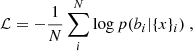 (6)
(6)
where N is the number of instances in the dataset. The inference is then performed by sampling the Gaussian base distribution and pushing these samples forward through the conditional transformation, parameterized by the input features ({x}), to give the posterior samples. See some examples of the use of NFs in astrophysics in, for example, Lovell et al. (2023), Sun et al. (2024), and Sun et al. (2025).
For higher-dimensional conditioned outputs, we employ neural spline autoregressive flows to jointly predict multiple galaxy properties conditioned on the set of halo and environment properties. The model is implemented using the Pyro library (Bingham et al. 2018).
3.2. Evaluation metrics
When assessing the performance of a ML model, it is essential to quantify how close the predicted values (ypred) are to the true ones (ytrue). This can be achieved using a set of evaluation metrics. In this work, we evaluate the performance of each model on the test set using three metrics: the Pearson correlation coefficient (PCC), the Kolmogorov–Smirnov test (K–S test), and the Wasserstein distance (WD). These metrics provide distinct but complementary perspectives: the PCC estimates linear correlation, the K–S test evaluates distributional similarity, and the WD measures global similarity between the entire predicted and true distributions.
The PCC, defined in Eq. (7) below, provides a normalized measure of covariance, yielding values between −1 and 1. It quantifies the degree of linear correlation between the predicted and true values, where +1 indicates a perfect positive linear relation and −1 a perfect negative one:
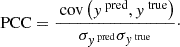 (7)
(7)
A higher PCC value corresponds to a stronger agreement between predictions and targets in terms of linear trends.
For the 1D K–S test, we adopted the statistic D computed using the scipy.stats.ks_2samp function from the scipy.stats module (Virtanen et al. 2020). This statistic quantifies the maximum difference between the cumulative distribution functions (CDFs) of two distributions, f1(x1) and f2(x2), namely:
 (8)
(8)
where F1(x1) = CDF[f1(x1)] and F2(x2) = CDF[f2(x2)]. This test evaluates whether two samples are drawn from the same underlying distribution; larger D values indicate greater discrepancies between them. For the 2D K-S test, we used the (Taillon 2018) repository.
Finally, the WD (also known as the earth mover’s distance) is a measure of the similarity between two probability distributions. It can be interpreted as the minimum “cost” required to transform one distribution into the other through optimal transport. Given two probability distributions u and v, defined over ℛ, the one-dimensional Wasserstein distance is expressed as:
 (9)
(9)
where Γ(u, v) represents the set of all joint probability distributions π on ℛ × ℛ with marginals u(x) and v(x) (Ramdas et al. 2015; Virtanen et al. 2020). Intuitively, this formulation seeks the joint distribution π(x, y) that minimizes the expected distance between points x and y when the values (x, y) are sampled from π(x, y). The WD accounts for the global structure of the distributions, making it particularly sensitive to differences in both location and shape. Consequently, lower WD values indicate a better match between the predicted and true distributions. This metric is widely employed in optimal transport theory and generative modeling applications (e.g., Arjovsky et al. 2017). In this work, we compute the 1D WD using the SciPy library (Virtanen et al. 2020), and the 2D WD using Flamary et al. (2021).
These metrics (PCC, K-S test and WD) are evaluated using point estimates (i.e., ypred is directly compared to ytrue). Since NFs predict the full posterior, it is necessary to summarize the posterior into a single number. Then, for the NF model, we computed the metrics in two ways. First, ypred was taken as a single random realization selected from the sampled outputs. Second, we used the mean value on all realizations, denoted as “avg”.
To evaluate the accuracy and calibration of the probabilistic predictions produced by the NF model, we performed a Test of Accuracy with Ranked Posteriors (TARP8; Lemos et al. 2023), which quantifies whether the posterior distributions predicted by the model are statistically well calibrated, namely, whether the true values are contained within the predicted credibility intervals at the expected rates. This test can be found in Appendix A.
4. Correlation between features
It is expected that many of the properties that we analyze in this work display a certain degree of correlation between them, and also with respect to linear bias. We assess the degree of correlation among features using the PCC, which quantifies the linear relationship between pairs of properties. This constitutes an important step, as ML algorithms do not rely on prior physical assumptions. As a means of providing a general view of the data set, we evaluate here how each property relates to bi.
Figure 1 shows the correlation of each selected property with the individual galaxy bias across the entire halo mass range. As expected, the local environment exhibits a greater connection with galaxy clustering compared to the remaining properties, with δ8 being the property most strongly correlated with the bias. For the cosmic web distances, an anticorrelation is observed for all distances except for that to the nearest void. This behavior is not surprising, as we approach denser environments (e.g., filaments and nodes), the bias increases, whereas proximity to less dense regions leads to weaker clustering (Montero-Dorta & Rodriguez 2024; Wang et al. 2024; Rodríguez-Torres et al. 2016).
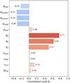 |
Fig. 1. Correlation of each selected property with individual galaxy bias, considering the entire mass range. Each bar is accompanied with the value of the linear correlation (PCC) between both features. |
Regarding the internal properties of halos, due to intrinsic scatter presented in the bias parameter, the correlation between this parameter and the internal properties of halos is also expected to be small9 (Paranjape et al. 2018; Han et al. 2019; Montero-Dorta et al. 2020; Balaguera-Antolínez et al. 2024), which is consistent with the values presented in Fig. 1. Interestingly, the internal property that presents the stronger correlation with galaxy bias is z1/2, instead of halo mass. This can be explained by the fact that the measurement, when taken globally for the entire population, is dominated by the more abundant low-mass halos, for which the dependence on halo mass is known to be weak (e.g., Tinker et al. 2010). Note also that there is an intrinsic connection between halo mass and age, which can be understood in terms of halo assembly history, where more massive halos–associated with stronger galaxy clustering–tend to form later through hierarchical merging.
The relation between halo mass and large-scale linear bias has been widely studied, both analytically and in simulations (Kaiser 1984; Bardeen et al. 1986; Mo & White 1996; Sheth & Tormen 1999; Sheth et al. 2001; Tinker et al. 2010). To explore additional dependencies, it is convenient to fix the halo mass. A practical approach to achieve this is by dividing the sample into narrow mass bins, as shown in Fig. 2, where the following bins are considered: 11.25 ≤ log10Mvir[h−1 M⊙]< 11.50; 12.05 ≤ log10Mvir[h−1 M⊙]< 12.30; 13.00 ≤ log10Mvir[h−1 M⊙]< 13.25; 14.02 ≤ log10Mvir[h−1 M⊙]< 15.02. All these bins span 0.25 dex, except for the most massive one, which is broader due to the limited number of objects in this region within the TNG300 simulation box. This simple exercise illustrates the power of individual bias to capture correlations at fixed halo mass, an effect commonly referred to as secondary halo bias (or halo assembly bias). The complete set of correlations between all features can be seen in the correlation matrices of Fig. B.1 in Appendix B.
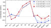 |
Fig. 2. Correlation coefficient between bi and each selected feature within four different halo mass bins. The bins span 0.25 dex, except for the most massive bin. |
At fixed halo mass, the correlation between the individual galaxy bias and halo mass increases for the most massive bin, consistent with the bias–mass relation. Furthermore, δ8 remains the property most strongly correlated with galaxy bias across all mass bins. As halo mass increases, the correlation between galaxy clustering and the formation redshift of the host halos decreases, whereas the opposite trend is observed for the spin, consistent with the well-known halo assembly bias and spin bias trends, respectively (see, e.g., Sato-Polito et al. 2019). In addition, decreasing halo mass strengthens the correlation between individual galaxy bias and proximity to different cosmic web structures, except for voids, in agreement with Montero-Dorta & Rodriguez (2024).
The trends observed in both Figures 1 and 2 are consistent with theoretical expectations and previous studies (see, e.g., Sato-Polito et al. 2019; Han et al. 2019; Paranjape et al. 2018; Alam et al. 2019; Montero-Dorta et al. 2020; Montero-Dorta & Rodriguez 2024; Balaguera-Antolínez et al. 2024), and form the foundation of the predictions of this work, as we want to test whether the different ML algorithms employed can successfully capture the underlying physical relationships among the various features. In addition, we also address feature importance using permutational feature importance in Sect. 5.2, allowing us to compare the relevance assigned by each model with the trends identified in this correlation analysis.
5. Predicting galaxy bias
5.1. Training procedure and model optimization
From the total sample of 174 607 objects used in this analysis, 58% were assigned to the training set, 30% to the test set, and 12% to the validation set. To determine the optimal architecture of each model, we employed the OPTUNA framework (Akiba et al. 2019) to perform Bayesian optimization using the Tree-structured Parzen Estimator (TPE; Bergstra et al. 2011), with 100 trials per model.
For the RF, the explored hyperparameters included the number of trees in the forest (n. estimators), the maximum depth of the trees (max. depth), the minimum number of samples required to split an internal node (min. samples split), and the maximum number of leaf nodes allowed (max. leaf nodes). The final set of hyperparameters corresponded to the configuration that achieved the lowest MSE on the validation set.
For the NN, we optimized the number of hidden layers, the layer sizes (i.e., number of nodes per layer), the activation function, the learning rate of the Adam optimizer, and the dropout rate. For the activation function, we considered ReLU, SiLU and LeakyReLU during the optimization process, with the latter yielding the best performance. Similarly, for the NF model, we explored the number of hidden layers, layer sizes, number of spline segments (bins), and batch size, and we sampled 1000 realizations from the learned conditional probability distributions. For both NN and NF models, the final hyperparameters were selected as those yielding the lowest value of the corresponding loss function (see Sect. 3.1) in the validation set. The final set of hyperparameters for the three models are presented in Tables 1, 2, and 3.
Explored hyperparameters for the RF.
Explored hyperparameters for the NN.
Explored hyperparameters for the NF.
5.2. Model comparison
Figure 3 presents the predictions from the three models compared to the true values. The top row shows the distributions of the predicted and true individual galaxy bias values for each model, while the bottom row displays scatter plots of predicted versus true values, color-coded by normalized density, which was estimated using Gaussian kernel density estimation (KDE) implemented through the scipy.stats.gaussian_kde function (Virtanen et al. 2020).
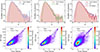 |
Fig. 3. Performance of each model in predicting the individual galaxy bias. The top row shows the true bias values distribution (in pink), along with the predictions from each model in different colors. The NF predictions present both a random realization (NF) and the expected value across the entire sample of realizations (NF Mean). The bottom row displays scatter plots comparing the predicted values (by each model) as a function of the true values, colored by normalized density. Notably, the bottom-right plot emphasizes the use of the NF random realization. The black dashed lines represent the ideal case where predicted values match the true values. |
It is evident that the deterministic models (RF and NN) are unable to closely reproduce the tails of the true bias values histogram, while increasing their precision in the high-density regions where most galaxies are found (see the top row of Fig. 3). This behavior is consistent with the corresponding scatter plots (bottom row of Fig. 3), where regions of higher normalized density lie closer to the ideal one-to-one relation, while other regions are more dispersed or deviate from the black dashed line.
For the generative model, selecting a single realization10 per galaxy reproduces the true bias values distribution more faithfully (see the purple line in the top row of Fig. 3). In contrast, taking the mean value across the entire sampled catalog for each galaxy fails to accurately reproduce the histogram of true values, as it approximates a deterministic model (i.e., the resulting distribution, shown in crimson in Fig. 3, has a similar shape to those of the NN and RF). This is the same behavior observed in the halo–galaxy connection previously identified and addressed in de Santi et al. (2022) using the SMOGN augmentation technique, and in Rodrigues et al. (2023, 2025) using binning classification schemes with NNs and generative models such as NFs. In Fig. 3, both cases (random realization and expected value) are shown alongside the true distribution, while the scatter plot corresponds to the single random realization case (purple line in the histogram).
We also computed the evaluation metrics described in Sect. 3.2 for each model on the test set to enable a quantitative comparison. The results for the deterministic estimators are presented in Table 4, while those for the probabilistic approach are listed in Table 5. In the latter, “avg” refers to metrics computed using the mean values, whereas the metrics without “avg” correspond to the case in which a single realization is selected.
Metric values for each single-point estimator (RF and NN).
Metric values for the probabilistic approach (NF).
For the deterministic models, RF exhibits slightly better performance than the NN across all three evaluation metrics, indicated by a higher PCC and lower values of the K–S test and WD. In the case of the NF model, when considering a single random realization, both the K–S test and the WD indicate that the predicted and true distributions are remarkably similar. This can be observed by comparing the pink histogram and the purple line in Fig. 3, demonstrating the ability of this probabilistic approach to accurately reproduce the true individual bias distribution.
However, selecting a single random realization from the NF-predicted conditional distributions also results in a low PCC value. This is evident in the corresponding scatter plot in Fig. 3, where the values are widely spread around the ideal case (black dashed line). Nevertheless, this scatter is highly symmetric, indicating that the model does not exhibit a systematic tendency to overestimate or underestimate the bias values, and that it is able to capture the global behavior of the data. When the expected value over the full set of 1000 sampled realizations is computed, the PCC increases and, when considering all three evaluation metrics, the model achieves a performance comparable to that of the RF.
Altogether, these results suggest that, although both deterministic models are robust in terms or their predictive capability, their predictions remain less accurate, capturing well the mean but not the width of the distributions. Their performance could be likely due to the intrinsic stochasticity of the bias parameter, reinforcing the notion that probabilistic methods are better suited for modeling and reproducing galaxy bias.
We also examined the relative impact of each input feature for the three ML algorithms used to predict galaxy bias. To this end, we employed permutation feature importance (PFI), performing 50 permutations per feature for each model on the test set. This method quantifies the contribution of an individual feature by measuring the degradation in the performance of the model when the relationship between that feature and the target is “broken”. A key advantage of PFI is that it is model-agnostic, allowing it to be applied consistently across different algorithms.
In this section, we consider a feature to be important when its PFI value is high, meaning that shuffling its values leads to a significant decrease in the performance of the model, in other words, the model strongly depends on that feature to make accurate predictions. The full set of importance values for each model is listed in Table 6, where the values are normalized such that the total importance for each model sums to unity.
Feature importance values for the three ML models.
All three models identify environmental properties as more relevant than the internal properties of the halos for predicting galaxy bias. In particular, δ8 emerges as the most influential feature, in agreement with the correlation analysis presented in Sect. 4, and exhibits a significantly higher importance than the remaining variables. This pronounced difference between the importance of δ8 and that of the other features further suggests that the models could potentially achieve acceptable predictive performance using only this single property.
Some features exhibit negative importance values, indicating that the performance of the model slightly improves when those variables are shuffled. This behavior suggests that such features do not contribute meaningful information to the predictions and may instead act as noise, and could therefore be discarded in future analyses. It is important to note that, because δ8 has such a strong impact, even when other features are permuted the algorithms still count on δ8, which provides most of the relevant information.
As shown in Fig. B.1 in Appendix B, there is a level of correlation among the features within each selected bin. In particular, the parameters exhibiting the highest degree of linear correlation (i.e., larger PCC values across bins) are δ3, δ5, and δ8. Consequently, despite their individual correlations with galaxy bias, permuting a single feature may not lead to a significant degradation in model performance (i.e., its PFI value remains relatively small). This does not imply that these features are not physically connected to galaxy bias, but rather that their contribution can be captured by other inputs.
Finally, an interesting aspect of NFs is that this technique enables the prediction of joint probability distributions. While deterministic estimators can also model such distributions, they generally do so with less fidelity than generative methods. To complement our analysis, we predicted pairs of properties and examined the performance of NFs in reproducing the scatter in these relations. As shown in Appendix C, NFs successfully reproduce the scatter in the bias–stellar mass and bias–color relations, yielding a 2D K–S statistic of 0.017 and a 2D WD of 0.030 for the bi–log10(M*[h−1 M⊙]) relation, and a 2D K–S statistic of 0.029 and a 2D WD of 0.052 for the bi–(g − i) relation. This scatter at fixed stellar mass and color reflects the intrinsic complexity of the physical processes governing halo and galaxy formation and evolution.
5.3. Individual probability distributions
One of the most useful features of NFs is their probabilistic treatment of the predicted outputs, which is particularly well suited to modeling galaxy bias given its highly stochastic nature. The NF model learns a family of conditional probability distributions p(bi|{x}i), where i indexes individual galaxies and {x}i denotes the set of selected input properties used to predict the individual bias of the galaxy (see Sect. 2). This approach enables us to model, for each galaxy in the sample, a full probability distribution of bias values rather than a single point estimate. We refer to these as individual probability distributions, and their shape depends on the selected input features. These distributions–examined in detail in this section–are obtained by sampling 1000 realizations per galaxy from the learned conditional model.
The shape of these individual probability distributions is sensitive to the choice of input properties, varying according to the information provided to the model. To explore this dependence, we compare the impact of two representative inputs: an internal halo property with low importance according to Table 6, being this λhalo, and the most influential feature, δ8. Using the same NF architecture exhibited in Table 3, we trained the model three times: (i) using only λhalo, (ii) using only δ8, and (iii) using the full set of selected properties. Figure 4 shows an example of the resulting individual bias distribution for the same randomly chosen galaxy under these different input configurations in purple, the blue dash line corresponds to the true bias value of the same galaxy, while the cyan distributions correspond to the true individual bias values histograms for the entire test set (as shown in pink in Fig. 3).
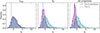 |
Fig. 4. Individual probability distributions (in purple) for one random galaxy in the sample obtained with the NF model trained with three different inputs. The left panel corresponds to the predicted values using λhalo as input, the center panel to the case only using δ8 as input while the right panel to the case using the complete set of properties described in Sect. 2. The blue dashed line corresponds to the true individual bias value of the galaxy (bi = −1.19), while the cyan distributions show the true bias values as shown in pink in Fig. 3. |
We find that when using features with low predictive power, such as λhalo, and therefore limited information content, the NF tends to reproduce a distribution similar to the overall distribution of the true bias values (see the left panel in Fig. 4), meaning that the model is unable to meaningfully constrain the conditional distributions on a per-object basis, particularly in the tails. This behavior arises because the conditioner network is unable to infer much information from this single property and therefore outputs similar spline parameters for all galaxies, resulting in nearly identical conditional distributions (p(bi|λhalo)). This effect becomes progressively less pronounced as more informative features are introduced, such as δ8, and is further mitigated when additional properties are included, as the model can extract more information from the inputs to infer object-dependent spline parameters and better constrain the conditional distributions, leading to variations in the shapes of these distributions that reflect the differences between the galaxies.
It is noteworthy that, regardless of the chosen input features for the generative model, selecting a single random realization from the full set of samples yields an overall distribution of bias values that closely matches the true one, as shown in the top panel of Fig. 5.
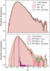 |
Fig. 5. Predicted individual probability distributions obtained with the NF model when using different input properties (only λhalo in purple, only δ8 in crimson, and the full set of halo and environmental properties in green). The top panel shows the distributions obtained when considering one random realization from the entire set of sampled values from the conditional probability distributions, while the bottom panel shows the case when taking the mean values of the individual probability distributions of each galaxy. |
However, caution must be exercised, as predictions for individual galaxies can be inaccurate when the input features are weakly informative, which is clearly visible when taking the mean value across all sampled realizations. This behavior is illustrated in the bottom panel of Fig. 5, where the contrast between models trained with less informative versus more influential features is evident. In particular, conditioning only on λhalo leads to mean values that cluster around the global average, producing the narrow peak observed in the figure (purple line).
Since NFs can be used to produce bias distributions for individual objects, it is interesting to evaluate how the internal variance of specific galaxy populations can be recovered. To this end, we placed galaxies in the color–stellar mass plane (features that were not predicted in this case) divided into 15 × 15 pixels, as shown in Fig. 6, where only pixels containing 30 objects or more were considered. For the true bias values, we computed the interquartile range (IQR) of the bias distribution for all objects within each pixel. For the predicted values, we used the full set of properties listed in Sect. 2 as input. Since in this case each galaxy in a pixel has its own bias distribution, we calculated the IQR for each individual distribution and then took the mean of all these IQR values. This mean IQR corresponds to the color scale shown for the predicted case in Fig. 6.
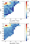 |
Fig. 6. 2D colormap of the IQR of the bias distributions per pixel. Each plot is divided into a 15 × 15 grid, and only pixels containing 30 objects or more are considered. The top panel shows the IQR of the true bias values for all objects within each pixel, while the bottom panel displays the mean IQR obtained by averaging the IQRs of the individual bias distributions of the galaxies contained in each pixel. |
The first notable result is the clear trend of the IQR increasing diagonally toward the red, low-mass corner of the parameter space, in both the real and the predicted case, which exhibit similar range of IQR values according to Fig. 6. To visualize this comparison more clearly, Fig. 7 displays a scatter plot of the predicted mean IQR as a function of the true IQR, along with the corresponding error bars, representing the standard deviation of the predicted IQR within each pixel. Although some discrepancies between the two cases exist, they follow the same general trend: the larger the dispersion in the data, the larger the predicted one. This result demonstrates that NFs can effectively capture the scatter of the bias parameter when using halo and environmental features as input, representing an important step toward characterizing its stochastic nature.
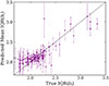 |
Fig. 7. Scatter plot of the predicted mean IQR as a function of the true IQR. Each purple dot represents a pixel (see Fig. 6), and the error bars correspond to the standard deviation of the predicted IQR within each pixel. The black dashed line indicates the ideal one-to-one relation (x = y), where the predicted and true IQRs are equal. |
6. Summary and conclusions
In this work, we present a ML framework aimed at reproducing the bias of galaxies as a function of internal halo properties and environmental diagnostics, as well as information on the location of galaxies within the cosmic web provided by DisPerSE. One of the main innovations of this framework is the adoption of the prescription of Paranjape et al. (2018) and Balaguera-Antolínez et al. (2024) to assign an individual bias value to each galaxy in the TNG300 hydrodynamical simulation, allowing us to incorporate bias into the ML machinery as an additional object-by-object property. We subsequently apply three different ML algorithms: two deterministic single-point estimators (a random forest regressor and a single-output neural network) and one probabilistic approach (normalizing flows) to predict the individual bias values following the methodologies of de Santi et al. (2022) and Rodrigues et al. (2023, 2025). The performance of all models is compared using three complementary evaluation metrics: the Pearson correlation coefficient, the Kolmogorov–Smirnov test, and the Wasserstein distance. Finally, we study the individual conditional probability distributions provided by the NF and analyze the ability of this generative method to reproduce the intrinsic variance of the bias parameter. The main conclusions of this paper can be summarized as follows:
-
Using a correlation analysis, we show that galaxy bias exhibits strong correlations with the overdensities measured on different scales (δ3, δ5, and δ8). These correlations strengthen with increasing scale, with δ8 emerging as the most strongly correlated feature. For sufficiently large R, both δR and bi probe a similar underlying quantity (Paranjape et al. 2018), which explains this tight connection (see also Pujol et al. 2017; Balaguera-Antolínez et al. 2023; Montero-Dorta & Rodriguez 2024). In order of decreasing strength, these correlations are followed by distances to cosmic-web critical points and, finally, by internal halo properties, with z1/2 being the most strongly correlated among them.
-
When analyzing the importance of each selected property in predicting galaxy bias across the different ML models, we find that all three models also identify δ8 as the most important feature, followed by δ5. Overall, the models are consistent with our correlation analysis in indicating that the environment has a greater impact on predicting the individual galaxy bias than the internal halo properties. The most notable difference is that δ3 becomes mostly uninformative once the larger-scale overdensities are included in the analysis.
-
We have shown that deterministic estimators are inherently limited in their ability to reproduce the true galaxy bias distributions with high fidelity, given the stochastic nature of the halo-galaxy connection. Rodrigues et al. (2025) proposes generative models to address this problem, and our results also demonstrate that NFs provide an effective approach to predict galaxy bias. In the bias-only case, the model achieves a K-S statistic of 0.010 and a Wasserstein distance of 0.046, considering a random realization. When predicting joint probability distributions, the model reaches a 2D K-S statistic of 0.017 and a 2D WD of 0.030 for the bi–log10(M∗[h−1 M⊙]) relation, and a 2D K-S statistic of 0.029 and a 2D WD of 0.052 for the bi–(g − i).
-
We find that when conditioning the NF model on properties that exhibit little or no correlation with the individual galaxy bias, such as halo spin, the model struggles to properly constrain the conditional individual probability distributions. In this case, the NF lacks sufficient information to distinguish between galaxies and therefore the conditioner network assigns similar conditional distributions to all objects. In contrast, the predicted distributions change significantly as more informative inputs are included, particularly features that are strongly correlated with the bias and therefore have greater predictive power.
-
We demonstrate that the NF predictions capture the behavior of the dispersion of the real data in a color–mass diagram, by following the same trend: the larger the variance in the true values, the larger the predicted one. These results, combined with the 1D and 2D distributions, demonstrate that such techniques are well suited to recover the intrinsic scatter of galaxy bias, reflecting the underlying complexity of the physical processes driving halo and galaxy formation and evolution.
Although the performance of all employed methods reflects the inherent challenges associated with predicting stochastic parameters, the predictive capability of each model also depends on the choice of input features. This highlights the potential benefit of incorporating additional information in future work, for example by including more informative environmental diagnostics such as refined cosmic web classification schemes (Galárraga-Espinosa et al. 2023), more sophisticated anisotropy estimators (Riveros-Jara, in prep.), or more complete evolutionary information from merger trees (e.g., Jespersen et al. 2022). Additionally, it is important to note that the proposed methods were trained on a specific simulation (in this case, TNG300), and variations in subgrid physics or halo-finding algorithms may affect the inferred bias dependencies and, consequently, the model predictions. Assessing the robustness of the framework across different simulations would therefore be a valuable next step.
This work is expected to have important future applications. In particular, our results constitute a meaningful advancement to measure galaxy bias observationally using data from upcoming surveys, such as the Dark Energy Spectroscopic Instrument (DESI; DESI Collaboration 2016). A natural next step for the observational applicability of our work is to assess whether individual bias can be similarly recovered from observable quantities – such as galaxy properties, halo mass estimates, and environmental indicators – within realistic mock catalogs, while properly accounting for survey selection effects and geometry in the estimator. These catalogs would also play a fundamental role in disentangling and quantifying the contributions of different sources of stochasticity, including those emerging from instrumental and modeling uncertainties.
We expect that the presented approach, particularly its probabilistic formulation, can facilitate the incorporation of individual galaxy bias into observational cosmology as a complementary probe to standard population-based bias measurements. A further promising direction is to extend this methodology to mock catalog generation, treating individual bias as an additional tracer property predicted from the matter density field within approximate mock-generation methods (e.g., Scoccimarro & Sheth 2002; Manera et al. 2013; Monaco et al. 2013; Balaguera-Antolínez et al. 2023; Balaguera-Antolínez & Montero-Dorta 2024).
Acknowledgments
We thank the anonymous referee for their insightful comments, which have significantly improved the quality of this paper. CRJ aknowledges Ricardo Ñanculef and the Department of Informatics of the Universidad Técnica Federico Santa María (UTFSM) for the computational resources provided for this project. CRJ and ADMD acknowledge support from the UTFSM through the Proyecto Interno Regular PI_LIR_25_04. CRJ and ADMD acknowledge the constant support of the AstroGainz research group. ABA acknowledges the Servicio Público de Empleo del Gobierno de España. NSMS acknowledges partial support from the NSF CDSE grant AST-2408026 and the NASA TCAN grant 80NSSC24K0101. MCA acknowledges partial support from ANID BASAL project FB210003. NVNR’s work at Argonne was supported under the DOE contract DE-AC02-06CH11357.
References
- Abbas, U., & Sheth, R. K. 2006, MNRAS, 372, 1749 [Google Scholar]
- Abbas, U., & Sheth, R. K. 2007, MNRAS, 378, 641 [Google Scholar]
- Akiba, T., Sano, S., Yanase, T., Ohta, T., & Koyama, M. 2019, Optuna: A Next-generation Hyperparameter Optimization Framework [Google Scholar]
- Alam, S., Zu, Y., Peacock, J. A., & Mandelbaum, R. 2019, MNRAS, 483, 4501 [NASA ADS] [CrossRef] [Google Scholar]
- Angulo, R. E., Baugh, C. M., & Lacey, C. G. 2008, MNRAS, 387, 921 [NASA ADS] [CrossRef] [Google Scholar]
- Arjovsky, M., Chintala, S., & Bottou, L. 2017, Wasserstein GAN [Google Scholar]
- Artale, M. C., Zehavi, I., Contreras, S., & Norberg, P. 2018, MNRAS, 480, 3978 [NASA ADS] [CrossRef] [Google Scholar]
- Balaguera-Antolínez, A., & Montero-Dorta, A. D. 2024, A&A, 692, A32 [NASA ADS] [CrossRef] [EDP Sciences] [Google Scholar]
- Balaguera-Antolínez, A., Kitaura, F.-S., Alam, S., et al. 2023, A&A, 673, A130 [NASA ADS] [CrossRef] [EDP Sciences] [Google Scholar]
- Balaguera-Antolínez, A., Montero-Dorta, A. D., & Favole, G. 2024, A&A, 685, A61 [NASA ADS] [CrossRef] [EDP Sciences] [Google Scholar]
- Bardeen, J. M., Bond, J. R., Kaiser, N., & Szalay, A. S. 1986, ApJ, 304, 15 [Google Scholar]
- Behroozi, P., Wechsler, R. H., Hearin, A. P., & Conroy, C. 2019, MNRAS, 488, 3143 [NASA ADS] [CrossRef] [Google Scholar]
- Beltz-Mohrmann, G. D., Berlind, A. A., & Szewciw, A. O. 2020, MNRAS, 491, 5771 [NASA ADS] [CrossRef] [Google Scholar]
- Bergstra, J., Bardenet, R., Bengio, Y., & Kégl, B. 2011, in Advances in Neural Information Processing Systems, eds. J. Shawe-Taylor, R. Zemel, P. Bartlett, F. Pereira, & K. Weinberger (Curran Associates, Inc.), 24 [Google Scholar]
- Bingham, E., Chen, J. P., Jankowiak, M., et al. 2018, Pyro: Deep Universal Probabilistic Programming [Google Scholar]
- Bluck, A. F. L., Piotrowska, J. M., Goubert, P., et al. 2025, A&A, 700, A272 [NASA ADS] [CrossRef] [EDP Sciences] [Google Scholar]
- Borzyszkowski, M., Porciani, C., Romano-Díaz, E., & Garaldi, E. 2017, MNRAS, 469, 594 [NASA ADS] [CrossRef] [Google Scholar]
- Bose, S., Eisenstein, D. J., Hernquist, L., et al. 2019, MNRAS, 490, 5693 [CrossRef] [Google Scholar]
- Breiman, L. 2001, Mach. Learn., 45, 5 [Google Scholar]
- Bullock, J. S., Dekel, A., Kolatt, T. S., et al. 2001, ApJ, 555, 240 [NASA ADS] [CrossRef] [Google Scholar]
- Buser, R. 1978, A&A, 62, 411 [NASA ADS] [Google Scholar]
- Calderon, V. F., & Berlind, A. A. 2019, MNRAS, 490, 2367 [NASA ADS] [CrossRef] [Google Scholar]
- Carliles, S., Budavári, T., Heinis, S., Priebe, C., & Szalay, A. 2007, Photometric Redshift Estimation on SDSS Data Using Random Forests [Google Scholar]
- Chaves-Montero, J., & Hearin, A. 2020, MNRAS, 495, 2088 [NASA ADS] [CrossRef] [Google Scholar]
- Chuang, C.-Y., Jespersen, C. K., Lin, Y.-T., Ho, S., & Genel, S. 2024, ApJ, 965, 101 [Google Scholar]
- Coil, A. L., Newman, J. A., Cooper, M. C., et al. 2006, ApJ, 644, 671 [NASA ADS] [CrossRef] [Google Scholar]
- Contreras, S., Zehavi, I., Padilla, N., et al. 2019, MNRAS, 484, 1133 [NASA ADS] [CrossRef] [Google Scholar]
- Contreras, S., Angulo, R. E., & Zennaro, M. 2021a, MNRAS, 504, 5205 [CrossRef] [Google Scholar]
- Contreras, S., Chaves-Montero, J., Zennaro, M., & Angulo, R. E. 2021b, MNRAS, 507, 3412 [NASA ADS] [CrossRef] [Google Scholar]
- Dalal, N., White, M., Bond, J. R., & Shirokov, A. 2008, ApJ, 687, 12 [NASA ADS] [CrossRef] [Google Scholar]
- Davis, M., Efstathiou, G., Frenk, C. S., & White, S. D. M. 1985, ApJ, 292, 371 [Google Scholar]
- de Santi, N. S. M., Rodrigues, N. V. N., Montero-Dorta, A. D., et al. 2022, MNRAS, 514, 2463 [CrossRef] [Google Scholar]
- DESI Collaboration (Aghamousa, A., et al.) 2016, ArXiv e-prints [arXiv:1611.00036] [Google Scholar]
- Desjacques, V., Jeong, D., & Schmidt, F. 2018, Phys. Rep., 733, 1 [Google Scholar]
- Dolag, K., Borgani, S., Murante, G., & Springel, V. 2009, MNRAS, 399, 497 [Google Scholar]
- Dolatabadi, H. M., Erfani, S., & Leckie, C. 2020, Invertible Generative Modeling Using Linear Rational Splines [Google Scholar]
- Duckworth, C., Starkenburg, T. K., Genel, S., et al. 2020a, MNRAS, 495, 4542 [Google Scholar]
- Duckworth, C., Tojeiro, R., & Kraljic, K. 2020b, MNRAS, 492, 1869 [NASA ADS] [CrossRef] [Google Scholar]
- Durkan, C., Bekasov, A., Murray, I., & Papamakarios, G. 2019, Neural Spline Flows [Google Scholar]
- Efstathiou, G., Ellis, R. S., & Peterson, B. A. 1988, MNRAS, 232, 431 [Google Scholar]
- Engler, C., Pillepich, A., Joshi, G. D., et al. 2021, MNRAS, 500, 3957 [Google Scholar]
- Flamary, R., Courty, N., Gramfort, A., et al. 2021, JMLR, 22, 1 [Google Scholar]
- Galárraga-Espinosa, D., Garaldi, E., & Kauffmann, G. 2023, A&A, 671, A160 [NASA ADS] [CrossRef] [EDP Sciences] [Google Scholar]
- Gao, L., & White, S. D. M. 2007, MNRAS, 377, L5 [NASA ADS] [CrossRef] [Google Scholar]
- Gao, L., Springel, V., & White, S. D. M. 2005, MNRAS, 363, L66 [NASA ADS] [CrossRef] [Google Scholar]
- Genel, S., Vogelsberger, M., Springel, V., et al. 2014, MNRAS, 445, 175 [Google Scholar]
- Gu, M., Conroy, C., Diemer, B., et al. 2020, ApJ, submitted [arXiv:2010.04166] [Google Scholar]
- Hadzhiyska, B., Bose, S., Eisenstein, D., Hernquist, L., & Spergel, D. N. 2020, MNRAS, 493, 5506 [NASA ADS] [CrossRef] [Google Scholar]
- Hadzhiyska, B., Bose, S., Eisenstein, D., & Hernquist, L. 2021, MNRAS, 501, 1603 [Google Scholar]
- Han, J., Li, Y., Jing, Y., et al. 2019, MNRAS, 482, 1900 [NASA ADS] [CrossRef] [Google Scholar]
- Hartley, W. G., Wilkins, S. M., Conselice, C. J., et al. 2013, MNRAS, 431, 3045 [Google Scholar]
- Hearin, A. P., & Watson, D. F. 2013, MNRAS, 435, 1313 [Google Scholar]
- Jespersen, C. K., Cranmer, M., Melchior, P., et al. 2022, ApJ, 941, 7 [NASA ADS] [CrossRef] [Google Scholar]
- Jo, Y., & Kim, J.-H. 2019, MNRAS, 489, 3565 [Google Scholar]
- Johnson, J. W., Maller, A. H., Berlind, A. A., Sinha, M., & Holley-Bockelmann, J. K. 2019, MNRAS, 486, 1156 [CrossRef] [Google Scholar]
- Kaiser, N. 1984, ApJ, 284, L9 [NASA ADS] [CrossRef] [Google Scholar]
- Kingma, D. P., & Ba, J. 2017, Adam: A Method for Stochastic Optimization [Google Scholar]
- Kingma, D. P., Salimans, T., Jozefowicz, R., et al. 2017, Improving Variational Inference with Inverse Autoregressive Flow [Google Scholar]
- Kreisch, C. D., Pisani, A., Villaescusa-Navarro, F., et al. 2022, ApJ, 935, 100 [NASA ADS] [CrossRef] [Google Scholar]
- Law-Smith, J., & Eisenstein, D. J. 2017, ApJ, 836, 87 [Google Scholar]
- Lazeyras, T., Musso, M., & Schmidt, F. 2017, JCAP, 2017, 059 [Google Scholar]
- Lemos, P., Coogan, A., Hezaveh, Y., & Perreault-Levasseur, L. 2023, Sampling-Based Accuracy Testing of Posterior Estimators for General Inference [Google Scholar]
- Li, C., Kauffmann, G., Wang, L., et al. 2006, MNRAS, 373, 457 [Google Scholar]
- Li, Y., Mo, H. J., & Gao, L. 2008, MNRAS, 389, 1419 [NASA ADS] [CrossRef] [Google Scholar]
- Lovell, C. C., Hassan, S., Villaescusa-Navarro, F., et al. 2023, Machine Learning for Astrophysics, 21 [Google Scholar]
- Lucie-Smith, L., Peiris, H. V., Pontzen, A., & Lochner, M. 2018, MNRAS, 479, 3405 [NASA ADS] [CrossRef] [Google Scholar]
- Manera, M., Scoccimarro, R., Percival, W. J., et al. 2013, MNRAS, 428, 1036 [Google Scholar]
- Marinacci, F., Vogelsberger, M., Pakmor, R., et al. 2018, MNRAS, 480, 5113 [NASA ADS] [Google Scholar]
- McNaught-Roberts, T., Norberg, P., Driver, S. P., et al. 2014, MNRAS, 445, 2125 [Google Scholar]
- Meneux, B., Le Fèvre, O., Guzzo, L., et al. 2006, A&A, 452, 387 [NASA ADS] [CrossRef] [EDP Sciences] [Google Scholar]
- Mo, H. J., & White, S. D. M. 1996, MNRAS, 282, 347 [Google Scholar]
- Monaco, P., Sefusatti, E., Borgani, S., et al. 2013, MNRAS, 433, 2389 [NASA ADS] [CrossRef] [Google Scholar]
- Montero-Dorta, A. D., & Rodriguez, F. 2024, MNRAS, 531, 290 [NASA ADS] [CrossRef] [Google Scholar]
- Montero-Dorta, A. D., Artale, M. C., Abramo, L. R., et al. 2020, MNRAS, 496, 1182 [NASA ADS] [CrossRef] [Google Scholar]
- Montero-Dorta, A. D., Artale, M. C., Abramo, L. R., & Tucci, B. 2021a, MNRAS, 504, 4568 [Google Scholar]
- Montero-Dorta, A. D., Chaves-Montero, J., Artale, M. C., & Favole, G. 2021b, MNRAS, 508, 940 [NASA ADS] [CrossRef] [Google Scholar]
- Montero-Dorta, A. D., Rodriguez, F., Artale, M. C., Smith, R., & Chaves-Montero, J. 2024, MNRAS, 527, 5868 [Google Scholar]
- Montero-Dorta, A. D., Balaguera-Antolínez, A., Alfaro, I. G., et al. 2025a, A&A, 703, A58 [NASA ADS] [CrossRef] [EDP Sciences] [Google Scholar]
- Montero-Dorta, A. D., Contreras, S., Artale, M. C., Rodriguez, F., & Favole, G. 2025b, A&A, 695, A159 [NASA ADS] [CrossRef] [EDP Sciences] [Google Scholar]
- Musso, M., Cadiou, C., Pichon, C., et al. 2018, MNRAS, 476, 4877 [Google Scholar]
- Naiman, J. P., Pillepich, A., Springel, V., et al. 2018, MNRAS, 477, 1206 [Google Scholar]
- Navarro, J. F., Frenk, C. S., & White, S. D. M. 1997, ApJ, 490, 493 [Google Scholar]
- Nelson, D., Pillepich, A., Springel, V., et al. 2018, MNRAS, 475, 624 [Google Scholar]
- Nelson, D., Springel, V., Pillepich, A., et al. 2019, Comput. Astrophys. Cosmol., 6, 2 [Google Scholar]
- Papamakarios, G., Pavlakou, T., & Murray, I. 2018, Masked Autoregressive Flow for Density Estimation [Google Scholar]
- Paranjape, A., & Sheth, R. K. 2012, MNRAS, 419, 132 [Google Scholar]
- Paranjape, A., Hahn, O., & Sheth, R. K. 2018, MNRAS, 476, 3631 [NASA ADS] [CrossRef] [Google Scholar]
- Paszke, A., Gross, S., Massa, F., et al. 2019, PyTorch: An Imperative Style High-Performance Deep Learning Library [Google Scholar]
- Pedregosa, F., Varoquaux, G., Gramfort, A., et al. 2018, Scikit-learn: Machine Learning in Python [Google Scholar]
- Peel, A., Lalande, F., Starck, J.-L., et al. 2019, Phys. Rev. D, 100, 023508 [Google Scholar]
- Perez, N. R., Pereyra, L. A., Coldwell, G., et al. 2024, MNRAS, 528, 3186 [Google Scholar]
- Pillepich, A., Nelson, D., Hernquist, L., et al. 2018a, MNRAS, 475, 648 [Google Scholar]
- Pillepich, A., Springel, V., Nelson, D., et al. 2018b, MNRAS, 473, 4077 [Google Scholar]
- Planck Collaboration XIII. 2016, A&A, 594, A13 [NASA ADS] [CrossRef] [EDP Sciences] [Google Scholar]
- Pollack, J. E., Smith, R. E., & Porciani, C. 2012, MNRAS, 420, 3469 [NASA ADS] [CrossRef] [Google Scholar]
- Pujol, A., Hoffmann, K., Jiménez, N., & Gaztañaga, E. 2017, A&A, 598, A103 [NASA ADS] [CrossRef] [EDP Sciences] [Google Scholar]
- Qiu, L., Napolitano, N. R., & Borgani, S., et al. 2024, A&A, 687, A1 [NASA ADS] [CrossRef] [EDP Sciences] [Google Scholar]
- Ramakrishnan, S., Paranjape, A., Hahn, O., & Sheth, R. K. 2019, MNRAS, 489, 2977 [NASA ADS] [CrossRef] [Google Scholar]
- Ramdas, A., Garcia, N., & Cuturi, M. 2015, On Wasserstein Two Sample Testing and Related Families of Nonparametric Tests [Google Scholar]
- Rodrigues, N. V. N., de Santi, N. S. M., Montero-Dorta, A. D., & Abramo, L. R. 2023, MNRAS, 522, 3236 [NASA ADS] [CrossRef] [Google Scholar]
- Rodrigues, N. V. N., de Santi, N. S. M., Abramo, R., & Montero-Dorta, A. D. 2025, A&A, 698, A3 [NASA ADS] [CrossRef] [EDP Sciences] [Google Scholar]
- Rodriguez, F., & Montero-Dorta, A. D. 2026, A&A, 707, A34 [NASA ADS] [CrossRef] [EDP Sciences] [Google Scholar]
- Rodríguez-Torres, S. A., Chuang, C.-H., Prada, F., et al. 2016, MNRAS, 460, 1173 [CrossRef] [Google Scholar]
- Salcedo, A. N., Maller, A. H., Berlind, A. A., et al. 2018, MNRAS, 475, 4411 [NASA ADS] [CrossRef] [Google Scholar]
- Sato-Polito, G., Montero-Dorta, A. D., Abramo, L. R., Prada, F., & Klypin, A. 2019, MNRAS, 487, 1570 [NASA ADS] [CrossRef] [Google Scholar]
- Schmidt, F., Jeong, D., & Desjacques, V. 2013, Phys. Rev. D, 88, 023515 [CrossRef] [Google Scholar]
- Scoccimarro, R., & Sheth, R. K. 2002, MNRAS, 329, 629 [NASA ADS] [CrossRef] [Google Scholar]
- Shao, H., Villaescusa-Navarro, F., Genel, S., et al. 2022, ApJ, 927, 85 [NASA ADS] [CrossRef] [Google Scholar]
- Sheth, R. K., & Tormen, G. 1999, MNRAS, 308, 119 [Google Scholar]
- Sheth, R. K., & Tormen, G. 2004, MNRAS, 350, 1385 [NASA ADS] [CrossRef] [Google Scholar]
- Sheth, R. K., Mo, H. J., & Tormen, G. 2001, MNRAS, 323, 1 [NASA ADS] [CrossRef] [Google Scholar]
- Shi, J., Wang, H., Mo, H., et al. 2020, ApJ, 893, 139 [Google Scholar]
- Skibba, R. A., Bamford, S. P., Nichol, R. C., et al. 2009, MNRAS, 399, 966 [NASA ADS] [CrossRef] [Google Scholar]
- Sousbie, T. 2011, MNRAS, 414, 350 [NASA ADS] [CrossRef] [Google Scholar]
- Springel, V. 2010, MNRAS, 401, 791 [Google Scholar]
- Springel, V., White, S. D. M., Tormen, G., & Kauffmann, G. 2001, MNRAS, 328, 726 [Google Scholar]
- Springel, V., Pakmor, R., Pillepich, A., et al. 2018, MNRAS, 475, 676 [Google Scholar]
- Stiskalek, R., Bartlett, D. J., Desmond, H., & Anbajagane, D. 2022, MNRAS, 514, 4026 [Google Scholar]
- Stücker, J., Pellejero-Ibáñez, M., Angulo, R. E., Maion, F., & Voivodic, R. 2025, A&A, 699, A197 [NASA ADS] [CrossRef] [EDP Sciences] [Google Scholar]
- Sullivan, J. M., Prijon, T., & Seljak, U. 2023, JCAP, 2023, 004 [Google Scholar]
- Sun, T.-Y., Xiong, C.-Y., Jin, S.-J., et al. 2024, Chin. Phys. C, 48, 045108 [Google Scholar]
- Sun, T.-Y., Shao, Y., Li, Y., et al. 2025, Commun. Phys., 8, 220 [Google Scholar]
- Taillon, G. 2018, 2DKS: Two-dimensional Kolmogorov–Smirnov Test Implementation, https://github.com/Gabinou/2DKS, accessed: 2025-11-08 [Google Scholar]
- Tinker, J. L., Robertson, B. E., Kravtsov, A. V., et al. 2010, ApJ, 724, 878 [NASA ADS] [CrossRef] [Google Scholar]
- Tucci, B., Montero-Dorta, A. D., Abramo, L. R., Sato-Polito, G., & Artale, M. C. 2021, MNRAS, 500, 2777 [Google Scholar]
- Villaescusa-Navarro, F., Anglés-Alcázar, D., Genel, S., et al. 2021, ApJ, 915, 71 [NASA ADS] [CrossRef] [Google Scholar]
- Virtanen, P., Gommers, R., Oliphant, T. E., et al. 2020, Nat. Methods, 17, 261 [Google Scholar]
- Vogelsberger, M., Genel, S., Springel, V., et al. 2014a, Nature, 509, 177 [Google Scholar]
- Vogelsberger, M., Genel, S., Springel, V., et al. 2014b, MNRAS, 444, 1518 [Google Scholar]
- Wang, Y., Yang, X., Mo, H. J., et al. 2008, ApJ, 687, 919 [NASA ADS] [CrossRef] [Google Scholar]
- Wang, L., Weinmann, S. M., De Lucia, G., & Yang, X. 2013, MNRAS, 433, 515 [NASA ADS] [CrossRef] [Google Scholar]
- Wang, K., Avestruz, C., Guo, H., Wang, W., & Wang, P. 2024, MNRAS, 532, 4616 [NASA ADS] [CrossRef] [Google Scholar]
- Wechsler, R. H., & Tinker, J. L. 2018, ARA&A, 56, 435 [NASA ADS] [CrossRef] [Google Scholar]
- Wechsler, R. H., Zentner, A. R., Bullock, J. S., Kravtsov, A. V., & Allgood, B. 2006, ApJ, 652, 71 [NASA ADS] [CrossRef] [Google Scholar]
- White, S. D. M., & Rees, M. J. 1978, MNRAS, 183, 341 [Google Scholar]
- Zehavi, I., Zheng, Z., Weinberg, D. H., et al. 2011, ApJ, 736, 59 [NASA ADS] [CrossRef] [Google Scholar]
- Zhai, Z., Percival, W. J., & Guo, H. 2023, MNRAS, 523, 5538 [Google Scholar]
In this expression, Phm(k) and Pmm(k) represent the halo-matter and matter-matter power spectra, respectively.
For simplicity, by stochasticity in this context we mean the intrinsic variance in the sample, once the different properties employed to reproduce the bias are taken into account.
The catalog can be directly downloaded from the TNG webpage. It can also be accessed from the GitHub link github.com/Chris-Duckworth/disperse_TNG
The assignment of individual galaxy bias has been performed using the CosmiCCcodes library at https://github.com/balaguera/CosmicCodes. A comprehensive derivation and interpretation of Eq. (3) can be found in Paranjape et al. (2018).
See Balaguera-Antolínez & Montero-Dorta (2024) for an inverse approach to the one described here, in which bias is used to assign halo properties in a probabilistic manner without relying on ML.
This test only applies for generative methods.
Montero-Dorta et al. (2020) showed that, albeit small, these correlations are enough to produce significant level of galaxy assembly bias, understood there as the secondary dependencies of galaxy bias at fixed halo mass.
Each realization is obtained by drawing one sample from the conditional distribution p(bi|{x}i). Fixing a single realization corresponds to one possible draw from the population-level distribution.
In this context, it is straightforward to extend our framework to predict secondary bias.
Appendix A: Coverage test
In order to assess the accuracy of the NF predictions, we performed a coverage test utilizing the TARP test. The coverage test evaluates the accuracy and calibration of probabilistic predictions by verifying whether the estimated posterior distributions correctly contain the true values at the expected credibility levels.
For each data point, many samples are drawn from the predicted posterior and compared to the true value from the simulation. The test measures the expected coverage probability (ECP) of credible regions at different credibility levels. If the posterior estimator is accurate, the empirical coverage should match the nominal credibility, yielding a one-to-one relation between coverage and credibility. Deviations from this diagonal indicate miscalibration: under-coverage signals overconfident or biased posteriors, while over-coverage indicates underconfident or overly broad predictions. A more detailed description of this test can be found in Rodrigues et al. (2025).
Figure A.1 shows the coverage test for the bias-only (1D case) predictions made with the NF model on the test set, suggesting our model is well calibrated, as it only presents small deviations from the one-to-one expected correspondence.
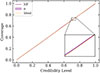 |
Fig. A.1. TARP coverage test for the 1-D case predictions with NF. The dashed orange line corresponds to the ideal one-to-one relation. The purple line exhibits the mean TARP for the model while the purple area covers one σ around the mean value. |
Appendix B: Correlation between features
One of the main advantages of adopting an object-by-object prescription to estimate the large-scale linear bias for each galaxy in a given sample (in this work, within the TNG300 simulation box) is that it allows us to disentangle its dependence on various properties, such as those related to the host halos and the local environment. In this work, we begin by analyzing how each property in the catalog correlates with the individual galaxy bias (bi), as shown in Fig. 1 and Fig. 2 for different halo mass bins. However, there are additional interesting relations among the selected properties that may be of interest to the reader and/or could be explored in future studies using the same techniques proposed here. For this reason, to complement the analysis presented in Sec. 4, here we describe the full correlation matrices in Fig. B.1, which show the linear correlations within the four distinct halo mass bins described in Sec. 4. In this appendix, we focus on the relationships among the features excluding bi, as the correlations involving the bias are already discussed.
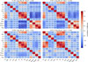 |
Fig. B.1. Complete correlation matrices for the four different mass bins presented in Fig. 2. Each plot shows the linear correlation between all features within the given mass bin. |
A notable trend in Fig. B.1 is the evolution of the correlation between the overdensities (δ3, δ5, and δ8) and the distances to critical points (dnode, dsaddle1, dsaddle2, and dskel). For the lower mass bins, these correlations are predominantly negative, whereas they shift toward positive values as the halo mass increases. This behavior suggests a mass-dependent correlation between the overdensities and the distances to critical points, which becomes more pronounced for more massive halos. In contrast, no clear trend is observed in the correlation between the overdensities and the distance to the nearest void (dmin).
Small variations are found in the correlations involving z1/2 and c200, which increase up to the second mass bin and then decrease for higher masses. A similar behavior is observed for their anticorrelation with the halo spin parameter.
Appendix C: Multiproperty predictions
Following the approach of Rodrigues et al. (2023, 2025), we jointly predict two pairs of properties as relevant examples: (i) the individual galaxy bias and stellar mass (p({bi, M*}|{x}i), and (ii) the individual galaxy bias and galaxy color (p({bi, g − i}|{x}i), adopting the same architecture presented in Table 3. These choices are motivated by two main considerations. First, both properties are observationally measurable. Second, the stellar mass of a galaxy is strongly correlated with the mass of its host halo, and galaxy color is linked to its accretion history (Hearin & Watson 2013; Wechsler & Tinker 2018; Behroozi et al. 2019; Chaves-Montero & Hearin 2020; Montero-Dorta et al. 2021b).
The predictions for both cases are presented in Fig. C.1, obtained by selecting a single random realization from the sampled catalog. Here, the main panels display the predicted values, color-coded by normalized density, while the contour lines represent the density of the true values from the catalog. The panels located above and to the right of each main panel show the marginal density distributions for both the predicted (gray area) and true (black lines) values. All densities (both in the scatter plots and histograms) were estimated using Gaussian KDE from the scipy.stats module.
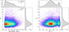 |
Fig. C.1. Joint probability distribution of both individual galaxy bias and stellar mass (left panel), as well as individual galaxy bias and galaxy color (right panel). The main panels show predicted values from one random realization, while black contour lines represent the density of the true values. The panels on the top and to the right of the main ones show the marginal density distributions for predicted values (gray) and true values (black lines). |
To quantify the difference between the predicted and true values for these multiproperty cases, we used the 2D K-S test and the 2D Wasserstein distance. The obtained values of each metric on the test set are listed in Table C.1.
Metric values for the NF multiproperty case.
The low values listed in Table C.1 demonstrate that NFs can effectively and accurately predict joint features, proving to be a powerful framework capable of predicting multiple correlated properties jointly rather than a single one. Although this study focuses on pairs of features, the method can be extended to include higher-dimensional joint predictions11 (see further discussion in Rodrigues et al. 2025).
A key result of this analysis is that NFs successfully reproduce the scatter in the bias–stellar mass and bias–color relations presented in Fig. C.1. This scatter at fixed stellar mass and color reflects the underlying complexity of the physical processes driving halo and galaxy formation and evolution.
All Tables
All Figures
|
Fig. 1. Correlation of each selected property with individual galaxy bias, considering the entire mass range. Each bar is accompanied with the value of the linear correlation (PCC) between both features. |
| In the text | |
|
Fig. 2. Correlation coefficient between bi and each selected feature within four different halo mass bins. The bins span 0.25 dex, except for the most massive bin. |
| In the text | |
|
Fig. 3. Performance of each model in predicting the individual galaxy bias. The top row shows the true bias values distribution (in pink), along with the predictions from each model in different colors. The NF predictions present both a random realization (NF) and the expected value across the entire sample of realizations (NF Mean). The bottom row displays scatter plots comparing the predicted values (by each model) as a function of the true values, colored by normalized density. Notably, the bottom-right plot emphasizes the use of the NF random realization. The black dashed lines represent the ideal case where predicted values match the true values. |
| In the text | |
|
Fig. 4. Individual probability distributions (in purple) for one random galaxy in the sample obtained with the NF model trained with three different inputs. The left panel corresponds to the predicted values using λhalo as input, the center panel to the case only using δ8 as input while the right panel to the case using the complete set of properties described in Sect. 2. The blue dashed line corresponds to the true individual bias value of the galaxy (bi = −1.19), while the cyan distributions show the true bias values as shown in pink in Fig. 3. |
| In the text | |
|
Fig. 5. Predicted individual probability distributions obtained with the NF model when using different input properties (only λhalo in purple, only δ8 in crimson, and the full set of halo and environmental properties in green). The top panel shows the distributions obtained when considering one random realization from the entire set of sampled values from the conditional probability distributions, while the bottom panel shows the case when taking the mean values of the individual probability distributions of each galaxy. |
| In the text | |
|
Fig. 6. 2D colormap of the IQR of the bias distributions per pixel. Each plot is divided into a 15 × 15 grid, and only pixels containing 30 objects or more are considered. The top panel shows the IQR of the true bias values for all objects within each pixel, while the bottom panel displays the mean IQR obtained by averaging the IQRs of the individual bias distributions of the galaxies contained in each pixel. |
| In the text | |
|
Fig. 7. Scatter plot of the predicted mean IQR as a function of the true IQR. Each purple dot represents a pixel (see Fig. 6), and the error bars correspond to the standard deviation of the predicted IQR within each pixel. The black dashed line indicates the ideal one-to-one relation (x = y), where the predicted and true IQRs are equal. |
| In the text | |
|
Fig. A.1. TARP coverage test for the 1-D case predictions with NF. The dashed orange line corresponds to the ideal one-to-one relation. The purple line exhibits the mean TARP for the model while the purple area covers one σ around the mean value. |
| In the text | |
|
Fig. B.1. Complete correlation matrices for the four different mass bins presented in Fig. 2. Each plot shows the linear correlation between all features within the given mass bin. |
| In the text | |
|
Fig. C.1. Joint probability distribution of both individual galaxy bias and stellar mass (left panel), as well as individual galaxy bias and galaxy color (right panel). The main panels show predicted values from one random realization, while black contour lines represent the density of the true values. The panels on the top and to the right of the main ones show the marginal density distributions for predicted values (gray) and true values (black lines). |
| In the text | |
Current usage metrics show cumulative count of Article Views (full-text article views including HTML views, PDF and ePub downloads, according to the available data) and Abstracts Views on Vision4Press platform.
Data correspond to usage on the plateform after 2015. The current usage metrics is available 48-96 hours after online publication and is updated daily on week days.
Initial download of the metrics may take a while.