


| Issue |
A&A
Volume 711, July 2026
|
|
|---|---|---|
| Article Number | A210 | |
| Number of page(s) | 16 | |
| Section | Numerical methods and codes | |
| DOI | https://doi.org/10.1051/0004-6361/202558408 | |
| Published online | 16 July 2026 | |
aim-resolve: Automatic identification and modeling for Bayesian radio interferometric imaging
1
Technical University of Munich, TUM School of Natural Sciences,
Boltzmannstr. 2,
85748
Garching,
Germany
2
Department of Astrophysics, Radboud University,
Heyendaalseweg 135,
Nijmegen,
6525 AJ,
The Netherlands
3
Max Planck Institute for Astrophysics,
Karl-Schwarzschild-Str. 1,
85748
Garching,
Germany
4
Technische Universität München (TUM),
Boltzmannstr. 3,
85748
Garching,
Germany
5
Faculty of Physics, Ludwig-Maximilians-Universität (LMU),
Geschwister-Scholl-Platz 1,
80539
Munich,
Germany
6
Kavli Institute for Particle Astrophysics & Cosmology (KIPAC), Stanford University,
Stanford,
CA
94305,
USA
7
German Center for Astrophysics,
Postplatz 1,
02826
Görlitz,
Germany
★ Corresponding author: This email address is being protected from spambots. You need JavaScript enabled to view it.
Received:
4
December
2025
Accepted:
4
May
2026
Abstract
Modern radio interferometers deliver large volumes of data containing high-sensitivity sky maps over wide fields of view. These large-area observations can contain various and superposed structures such as point sources, extended objects, and large-scale diffuse emission. To fully realize the potential of these observations, it is crucial to build appropriate sky emission models that separate and reconstruct the underlying astrophysical components. We introduce aim-resolve, an automatic and iterative method that combines the Bayesian imaging algorithm resolve with deep learning and clustering algorithms in order to jointly solve the reconstruction and source extraction problem. The method identifies and models different astrophysical components in radio observations while providing uncertainty quantification of the results. By using different model descriptions for point sources, extended objects, and diffuse background emission, the method efficiently separates the individual components and improves the overall reconstruction. We demonstrate the effectiveness of this method on synthetic image data containing multiple different sources. We further show the application of aim-resolve to an L-band (856–1712 MHz) MeerKAT observation of the radio galaxy ESO 137-006 and other radio galaxies in that environment. We observe a reasonable object identification for both applications, yielding a clean separation of the individual components and precise reconstructions of point sources and extended objects along with detailed uncertainty quantification. In particular, the method enables the creation of catalogs containing source positions and brightnesses and the corresponding uncertainties. The full decoupling of sky emission model and instrument response makes the method applicable to a wide variety of instruments or wavelength bands.
Key words: instrumentation: interferometers / methods: data analysis / methods: statistical / techniques: image processing
© The Authors 2026
 Open Access article, published by EDP Sciences, under the terms of the Creative Commons Attribution License (https://creativecommons.org/licenses/by/4.0), which permits unrestricted use, distribution, and reproduction in any medium, provided the original work is properly cited.
This article is published in open access under the Subscribe to Open model. This email address is being protected from spambots. You need JavaScript enabled to view it. to support open access publication.
1 Introduction
Modern and upcoming radio interferometers, notably the Australian Square Kilometre Array Pathfinder, MeerKAT, and the Square Kilometre Array (SKA), are leading to major improvements in radio astronomical imaging. These arrays are starting to produce large volumes of data containing high-sensitivity sky maps over wide fields of view (FOVs). These large-area observations often contain various and superposed structures such as point sources, extended objects, and large-scale diffuse emission. To fully realize the potential of these observations, it is crucial to build appropriate sky emission models that reconstruct and separate the underlying astrophysical components.
This is a challenging task for several reasons. In general, radio interferometric imaging is an underconstrained problem that requires some form of regularization. As the individual sources vary in both type and size, they cannot be sufficiently described by a single sky emission model. In addition, the exact locations of point sources and extended objects are often not known beforehand. Finally, the entire imaging process should be fully automated; this would allow it to be applied to new and unknown datasets. To solve these problems, we combined Bayesian imaging with object identification and source extraction to an automatic and iterative method named aim-resolve.
Determining the locations of individual objects, often referred to as source finding, is a well-known task in radio astronomy. A summary and comparison of different tools can be found in Hopkins et al. (2015). Recent advances in machine learning have enabled further improvements to source finding. In particular, convolutional neural networks (CNNs) have been successfully used to detect point sources (Lukic et al. 2019; Vafaei Sadr et al. 2019; Tilley et al. 2021) or to classify the morphology of radio galaxies (Bowles et al. 2021; Schmidt et al. 2022; Taran et al. 2023).
Most of these source finding algorithms run on images reconstructed using some variant of the CLEAN algorithm, originally proposed by Högbom (1974), which is a commonly employed imaging algorithm in radio interferometry, due to its computational efficiency and simplicity. Although it has been significantly improved over the last decades, in particular for diffuse emission, wide-field imaging, and spectral imaging (Schwab & Cotton 1983; Bhatnagar & Cornwell 2004; Cornwell 2008; Offringa & Smirnov 2017), CLEAN-based algorithms still have a few drawbacks. They do not output any uncertainty information, they often require manual guidance to ensure their stability, and CLEAN restored images often exhibit limited image quality and resolution (Arras et al. 2021; Terris et al. 2022). In addition, CLEAN can produce imaging artifacts, which often need to be excluded manually before or during the source finding process.
Many other imaging algorithms have been developed to improve these limitations. One large class are convex or noncon-vex optimization algorithms using sparsity-based regularizers, originally proposed by Wiaux et al. (2009). Recent examples of such algorithms (Birdi et al. 2019; Dabbech et al. 2022; Thouvenin et al. 2022) have led to improvements in terms of image fidelity and resolution compared to advanced versions of CLEAN. Repetti et al. (2019) proposed some form of uncertainty quantification for these methods.
A second large class of novel imaging algorithms builds on Bayesian inference. By accessing the posterior distribution, Bayesian imaging algorithms address the uncertainty quantification problem from first principles. Many Bayesian imaging algorithms (Cai et al. 2018; Tiede 2022) are based on posterior sampling techniques. The Bayesian imaging algorithm resolve1 (Junklewitz et al. 2016; Arras et al. 2019) employed in this work builds on variational inference (VI) for computational efficiency. Recent examples are Arras et al. (2022) applying resolve to Event Horizon Telescope (EHT) data and Roth et al. (2023) joining Bayesian imaging with directiondependent calibration. Arras et al. (2021) shows the enhancements of resolve compared to CLEAN, such as higher image fidelity, super-resolution, and uncertainty quantification of the results. However, the improvements come at the cost of higher computational effort. The recently presented fast-resolve algorithm (Roth et al. 2024) addresses this problem and significantly reduces the computational complexity compared to classical resolve, enabling Bayesian image reconstruction of large datasets similar to a MeerKAT wide-field observation.
resolve is built on the numerical information field theory (NIFTy2) Python package (Selig et al. 2013; Arras et al. 2019; Edenhofer et al. 2024), which relies on accurate VI algorithms yielding posterior samples of the reconstructed quantities. NIFTy allows us to build complex forward models and to separate different components during the reconstruction of the data. These features have already been successfully applied to X-ray and γ-ray observations separating point sources or even extended objects from a diffuse background (Scheel-Platz et al. 2023; Westerkamp et al. 2024; Eberle et al. 2026). Very recently, Guardiani et al. (2025) introduced a NIFTy-based method to automatically detect and model point sources in astronomical surveys using model latent-space information and applied it to X-ray data. However, the FOV and model parameters for the extended objects have been set manually in these examples. This becomes infeasible for a large number of extended components as they can occur in radio wide-field observations.
In aim-resolve, we utilize traditional deep learning and clustering algorithms to detect both point sources and extended sources in radio observations. The method first produces a preliminary reconstruction of the radio sky with fast-resolve. Next, it identifies point sources and extended objects within this reconstruction and uses the available information, such as the localization and brightness of the sources, to build a multicomponent sky model. By utilizing different model descriptions for different types of sources, the method successfully separates the individual sources from each other. The following joint optimization of the multi-component sky model with the data improves the overall reconstruction while providing uncertainty quantification of the results. The whole method is executed in an automatic and iterative manner.
The remaining paper is organized as follows. Section 2 discusses the imaging problem in radio interferometry and the corresponding measurement equation. In Sect. 3, we first describe the underlying tools used for modeling, optimization, and object identification, before we combine them to the iterative method of aim-resolve. In Sect. 4, we validate the method on synthetic radio data, and show its application to a MeerKAT radio wide-field observation.
2 Imaging in radio interferometry
For a general image reconstruction task with additive noise the measurement equation reads
 (1)
(1)
where d is the observed data, I is the image or signal to be reconstructed, R is the signal response mapping the image to the data, and n is an additive noise realization. The response function depends on the particular instrument.
In radio interferometry we do not measure the sky brightness distribution I directly. Instead, data from a large number of telescopes is combined to measure Fourier components of the sky brightness, often referred to as visibilities. For an ideal unpolarized interferometer the visibilities V are given by the radio interferometric measurement equation (Thompson et al. 2017)
![Mathematical equation: \mathcal{V}(u,v,w) = R\,I = \int \frac{I(l,m)}{n(l,m)} e^{-2\pi i [ul + vm + w(n(l,m) -1)]} dl \, dm,](/articles/aa/full_html/2026/07/aa58408-25/aa58408-25-eq2.png) (2)
(2)
where I(l, m) is the sky brightness distribution, (l, m, n(l, m) =  ) are the sky coordinates, and (u, v, w) are the relative positions of antenna pairs. We further assume uncorrelated Gaussian noise.
By combining Eqs. (1) and (2), one can easily generate model visibilities for given sky brightness distributions and noise statistics. However, directly inverting the operation is impossible as the data is corrupted by noise and is measured only at sparse locations in Fourier space. For this reason, several different images might be consistent with the same data. Solving this underconstraint problem requires additional regularization, for example through the incorporation of prior distributions.
3 Method
In this section, we introduce the iterative method of aim-resolve. The general approach has been outlined in Fuchs et al. (2025). We first give an overview over the frameworks and tools used within the method. This includes the setup of a flexible generative model that allows a full description of the radio sky (Sect. 3.1), followed by the utilized optimization algorithms of NIFTy and fast-resolve (Sect. 3.2). Next, we demonstrate how objects can be identified in a reconstruction using deep learning and clustering techniques (Sect. 3.3), and finally combine everything to the aim-resolve method (Sect. 3.4).
3.1 Modeling
resolve infers the posterior probability distribution P(I|d) of the sky brightness conditioned on the measured data, instead of using a point estimate. The posterior distribution can be expressed in terms of the evidence P(d), the likelihood P(d|I), and the prior distribution P(I) via Bayes’ Theorem:
 (3)
(3)
Because of the size and complexity of our imaging problem, we approximate the posterior using the optimization algorithms of NIFTy and fast-resolve, which are discussed in Sect. 3.2. In the next two subsections we set up a versatile and adjustable model for the full sky brightness distribution and formulate the underlying NIFTy prior models. We furthermore describe the likelihood assumed in resolve.
3.1.1 Sky description
As stated before, the observed radio sky often contains various different sources with widely varying physical properties. Therefore, a single sky emission model is not sufficient to describe all structures present in radio observations.
Especially diffuse emission and point sources have very different morphologies. For this reason, we use different prior models for point sources and extended objects. Previous applications of resolve followed similar approaches. For example, Arras et al. (2021) introduced a separate model for two point sources with known positions to improve the imaging of Cygnus A. In this work, we extend this ansatz to an arbitrary number of point sources whose locations are determined throughout our method.
In addition to the separation between extended objects and point sources discussed above, there is also a wide variety of extended sources. To address this, we introduce tile components, pointing to specific subparts of the signal field. Additionally, we incorporate a diffuse background component to capture any remaining objects and large-scale structures that are not represented by one of the tiles. Together with the point sources, the full forward model for the sky brightness distribution reads
 (4)
(4)
where Ib represents the diffuse background, Iit denotes N individual tile components, and Ipj signifies the M point sources. By pairing this model description with sensible prior distributions for the individual components, we can describe various structures and sources at different scales.
3.1.2 Prior models
We employ NIFTy to set up the prior models for the three different types of components. A central requirement for all prior models is positivity, as the observed flux in radio astronomy is strictly positive. Additionally, they must be able to model significant variations in sky brightness, which can span several orders of magnitude.
Nearly all continuous quantities, such as galaxies and large-scale diffuse emission, can be described as correlated structures. To capture this behavior, we describe these structures using Gaussian processes (GPs), which model correlations between nearby pixels represented by a power spectrum in Fourier space. As the exact correlation structure of a component is not known a priori, we use a nonparametric model for this power spectrum and infer it jointly with the GP. Further details of this correlation model can be found in Arras et al. (2022).
In general, we encode our prior models as standardized generative models (Knollmüller & Enßlin 2018), which map a set of standard normal distributed random variables {ξ} to the desired target distribution. To ensure the non-negativity of the diffuse model, we simply exponentiate the GP model to encode a correlated log-normal distribution
![Mathematical equation: I^{\text{d}}(\xi) = \exp{(\mathcal{F}^{-1} [\sqrt{P_\Psi (\xi_\Psi) }~ \xi_k ] )},](/articles/aa/full_html/2026/07/aa58408-25/aa58408-25-eq6.png) (5)
(5)
where F−1 is the inverse Fourier transform operator, and Pψ(ξψ) is the nonparametric power spectrum modeling the spatial correlations.
Since this model is quite flexible, we can utilize it to describe background and tile components by adjusting the hyperparameters. Thus, we can express each compact object with its individual correlation structure. For the tile components, we further multiply the output of the log-normal correlation model with a two-dimensional Gaussian with a learnable covariance, similarly to the prior model of Rüstig et al. (2024). This reduces the degeneracies in parameter space between the background and the tile components, and ensures that the tile components fall off to zero toward the edges. These tile components are then inserted to the specific subparts of the signal field.
While the correlation model works well with different kinds of extended objects, it has problems in describing point sources. In this work, we aim to predict the exact pixel locations of point sources throughout our method. Moreover, we are able to determine the flux of each detected point source. Thus, instead of having a point source prior everywhere in the image space, which would lead to a high degeneracy, we insert an individual model for each identified source j at its predicted pixel coordinates and describe its brightness with a log-normal distribution
 (6)
(6)
which maintains the necessary positivity constraint. It transforms the standard normal distributed random variables ξpj to a normal distribution with mean µj and standard deviation σj.
3.1.3 resolve likelihood
Following Arras et al. (2021), we assume Gaussian noise statistics with diagonal covariance N,  . The likelihood is therefore Gaussian as well, given by
 (7)
(7)
For numerical reasons, we work with the negative log-likelihood,
 (8)
(8)
where the dagger (†) denotes the complex conjugate transpose. We note that I is the full sky brightness model specified in Eq. (4) and may consist of a varying number of different components during the iterative method.
3.2 Optimization
Given the full model for the sky brightness distribution and the likelihood, we want to estimate the posterior distribution in Eq. (3). For radio interferometric data with millions of visibilities, we employ the fast-resolve optimization scheme, presented in Sect. 3.2.2. This algorithm relies on accurate VI algorithms of NIFTy, which are introduced first.
3.2.1 NIFTy posterior inference
In VI, we approximate the posterior distribution using a family of distributions by minimizing the Kullback–Leibler divergence between the approximation and the true distribution. In this work, we employ geometric variational inference (geoVI, Frank et al. 2021) to efficiently approximate the posterior distribution with a set of samples allowing us to produce reliable uncertainty estimates for the results.
In general, VI methods scale much better with the number of parameters compared to sampling techniques such as MCMC and HMC, making them still applicable to high-resolution imaging problems (Blei et al. 2017). However, they still involve many likelihood calls within the inference, which increases the computational costs if the evaluation of the likelihood is expensive. In resolve, each evaluation of the likelihood requires the computation of RI and thus the integral in Eq. (2). In practice, this boils down to computing a discrete non-uniform Fourier transformation. Although resolve relies on the parallelizable wgridder implemented in the ducc3 library to perform this operation, the evaluation of RI becomes computationally expensive for large datasets with millions of visibilities.
3.2.2 fast-resolve inference
To eliminate this bottleneck, Roth et al. (2024) introduced the fast-resolve algorithm with the aim of reducing the number of response evaluations. The basic idea is to perform most of the computations in image space by multiplying both sides of Eq. (1) with R†N−1 from the left. By approximating the response function of the new likelihood by a convolution with the point spread function of the interferometer and the application of the noise inverse with an appropriate noise kernel, the evaluation time of the new likelihood can be reduced significantly.
Inspired by the CLEAN algorithm, fast-resolve uses a major–minor cycle inference scheme. In the minor cycles, it optimizes the current estimate of the posterior distribution of the sky brightness using the above approximations. The major cycles then correct for approximation errors by applying the exact response function. For more detail on the exact inference scheme and the gained speedup refer to Roth et al. (2024).
3.3 Object identification
In order to build a full multi-component model (MCM), we need to predict the locations of both point sources and extended objects in a resolve reconstruction. There are three major challenges in this task. First, the number of objects is unknown before; second, we strive for a highly precise localization of the individual objects, especially the point sources; and third, the prediction should work on inputs with variable resolutions.
3.3.1 Semantic segmentation
We tackle these problems using semantic segmentation, which provides a detailed understanding of the image’s content at the pixel level by assigning labels to every pixel. We chose the U-Net architecture (Ronneberger et al. 2015) for our prediction network, which features an encoder–decoder structure with skip connections that enable the precise localization of features, while maintaining spatial details. Due to its fully convolutional architecture, it can even process inputs with different resolutions.
We set up the network in a way that it takes a reconstructed image as input and produces two output segmentation maps, indicating whether a pixel represents a point source or not, or whether it belongs to an extended object or not. After training the U-Net on synthetic image and label pairs, we can get fast predictions of the source locations when running our iterative method.
3.3.2 Training data
For the training data, we set up a generative model to produce synthetic images and labels at various resolutions. The images contain many different structures to resemble actual resolve reconstructions of radio wide-field observations.
To achieve this, we introduce some diffuse background emission in the middle of the FOV by multiplying the lognormal correlation model from Sect. 3.1.2 with a two-dimensional Gaussian. We generate extended objects that look like real radio galaxies by using part of the RadioGalaxyDataset4, a collection of several radio catalogs (Becker et al. 1995; Miraghaei & Best 2017; Gendre & Wall 2008; Gendre et al. 2010; Capetti et al. 2017b,a; Baldi et al. 2018; Proctor 2011), and add them to the background. We further add variable numbers of point sources and small extended objects at random locations. The point sources can be blurred over several pixels, since our correlation model cannot perfectly represent them. At the same time, we generate the two output segmentation maps using the pixel locations of the inserted point sources and compact objects, as well as the pixels occupied by the extended objects from the RadioGalaxyDataset images. A subset of the training data can be found in Fig. C.2.
3.3.3 Clustering
From the first output segmentation map of the U-Net, we can directly extract the number of point sources and their exact pixel locations. However, we only get a single output map, which can contain several extended objects. To discriminate between them, we employ density-based spatial clustering of applications with noise (DBSCAN) introduced by Ester et al. (1996). Compared to other clustering algorithms it does not require the number of clusters as input, and works well for data with clusters of similar density, which is the case for two-dimensional images. By setting a minimum cluster size, DBSCAN can additionally have a regulating role; for example, it can prevent blurred-out point sources from being misclassified as small extended objects.
3.4 Iterative procedure
We combine the modeling, optimization, and identification steps to the method aim-resolve in order to iteratively improve the reconstruction of the data. We set up a fully automatized pipeline using the snakemake workflow language (Mölder et al. 2021) to efficiently manage the sequence of the individual steps.
Figure 1 shows a visualization of aim-resolve, depicting the individual steps of the method. In step (0) we initialize the process, load the data and specify the desired resolution and FOV we wish to reconstruct. On the model site, we start with a single-component model (SCM), which consists solely of the background component from Sect. 3.1.1, and initialize its correlation model with rather wide and flexible hyper-parameter priors. After running the inference in step (d), we get a preliminary reconstruction of the data that serves as a starting point for our method, which iterates over the following steps:
- (a)
Detection: first, the trained U-Net is used to identify point sources and objects within the preliminary reconstruction. The point source positions can be extracted directly from the corresponding output segmentation map. To discriminate between the different extended objects, the clustering algorithm from Sect. 3.3.3 is applied to the corresponding output map.
- (b)
Modeling: this step determines the center of the contained object for each output cluster and draws a bounding box by adding a margin around it. Additionally, it extracts the flux of each point source and object from the previous reconstruction and sets the new model hyper-parameters accordingly. Using all the available information, it creates a model configuration file for the subsequent reconstruction iteration by adding the new components to the background model, yielding a MCM.
- (c)
Separation and pre-fit: before continuing the optimization on the data, the new model is fitted to the previous reconstructed image. This step is similar to the transition model introduced by Westerkamp et al. (2024). By masking the background at the locations of the detected components, this step efficiently separates the point sources and extended objects from the background. Next, the individual model components are fitted to the corresponding areas of the old reconstruction. We note that the transition saves computation time since the prefit on the previous reconstructed image does not involve any expensive response function. More details on this transition to the new model can be found in Appendix A.
- (d)
Reconstruction: the pre-fitted model serves as a starting point to continue the optimization on the data. With the new MCM, we now can create plots for each individual component separated from each other. Moreover, the components can be added together to compose an image of the full sky, thus allowing object detection in the next pipeline iteration.
The iterative pipeline is repeated multiple times for further refinement and stops once the reconstruction does not improve anymore. We note that we re-predict all point sources and extended objects at each detection iteration and set rather wide brightness priors on the added components. This ensures that potentially incorrectly identified components from the previous detection step are corrected or removed from the model and thus the overall reconstruction iteratively improves.
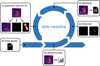 |
Fig. 1 Visualization of the iterative method of aim-resolve. Initialized with a single-component model (0), it generates a preliminary reconstruction of the data (d). It detects point sources and extended objects in the reconstruction (a) and adds the identified components, marked with crosses and boxes, to the existing background model (b). Next, it separates the components from the background and fits them to the previous reconstructed image (c), before it continues the optimization on the real data (d). This cycle is repeated multiple times for further refinement. |
4 Applications
We now demonstrate the applicability of our method. We first describe the training of the U-Net and its performance on unseen test data in Sect. 4.1. In Sect. 4.2, we validate our method on synthetic radio data before we finally apply it to real radio interferometric data in Sect. 4.3.
Performance of the U-Net.
4.1 Training of the U-Net
We use the generative model introduced in Sect. 3.3.2 to produce several training, validation, and testing datasets at various resolutions. All of them can contain some diffuse background emission, large radio galaxy-like objects, and up to 25 point sources and small extended components. The idea of differently resolved datasets is to first train the U-Net described in Sect. 3.3.1 on a dataset with a rather low resolution, which reduces the memory usage and allows faster training, and later fine-tune the U-Net on training data with a high resolution to achieve a good performance on high-resolution images.
Before the data is fed into the U-Net, we take the logarithm of the images and normalize them. Furthermore, we randomly flip and rotate the images and labels to allow different orientations of the radio galaxy-like objects within the images. We set up the UNet using the segmentation-models-pytorch5 package with a ResNet-50 encoder pre-trained on the ImageNet6 dataset, with one input channel and two output channels. We achieved the best results using a dice loss function, an adaptive moment estimation (Adam) optimizer, and a cosine annealing learning rate scheduler. For the first step, we train the U-Net on a dataset containing 10 000 images and labels with a resolution of 128 X 128. Afterward, we fine-tune the trained U-Net on the final resolution the neural network should operate on. We do this for two different resolutions, 512 X 512 and 1024 X 1024, with 1000 images and labels each.
To measure the performance of the network’s predictions, we use the mean intersection of union (mIoU). Unlike the pixelwise accuracy, mIoU aims to mitigate class imbalances and to take false positives into account. However, the per-dataset mIoU is biased toward large objects in the dataset. Our dataset shows exactly this size imbalance, since extended objects contain more pixels than point sources. Wang et al. (2023) propose using finegrained mIoU at the per-image level to address this problem. We first compute the mIoU score for each image i and each class c via
 (9)
(9)
where TP, FP, and FN represent true positives, false positives, and false negatives, respectively. Next, we average these scores first by image and then by class. The order of the averaging ensures that point sources and extended objects are given the same importance. Table 1 compares the fine-grained mIoU at the per-image level of several fine-tuned U-Nets on test datasets with different resolutions.
As expected, the U-Nets perform best on the resolution they are fine-tuned on. U-Net 512 and U-Net 1024 still perform acceptable on lower-resolution inputs due to the pre-training. Although the fine-tuning requires additional training steps, it considerably improves the performance with a fairly short additional training time. Of course, the training time increases when going to even higher resolutions.
Compared to just identifying the brightest pixels in a reconstruction by setting some cutoff value, the U-Nets can separate point sources from extended objects, which is not trivial for this dataset since a varying diffuse background can have a similar brightness as some of the objects and point sources can be blurred out.
4.2 Validation on synthetic data
To evaluate the performance and robustness of our proposed method, we validate the reconstruction pipeline on synthetic radio data. The main objectives of this validation are to verify that the combination of U-Net and clustering efficiently identifies and distinguishes different objects within a reconstruction, and that the MCM works in combination with a radio interferometric response and improves the overall reconstruction quality compared to a SCM.
For the synthetic data, we pick one sample from the test-512 dataset, apply the MeerKAT response function from Sect. 4.3 to it, and add Gaussian noise to the generated visibilities. The ground truth image is shown in Fig. 2. The selected example contains some diffuse background emission and two large radio galaxy-like objects with two lobes each, as well as 12 point sources and 25 small extended objects. Figure 2 further shows the naturally weighted dirty image, which we get by applying R†N−1 to the generated radio data. This serves as a starting point for the aim-resolve inference.
4.2.1 Reconstruction and identification
As described in Sect. 3.4, we first get a preliminary reconstruction of the noisy image data using the SCM and the fast-resolve algorithm. The initial hyper-parameters of the resolve correlation model are given in Table B.1. Using the UNet fine-tuned on the test-512 data and following the detection and modeling steps described in Sect. 3.4, aim-resolve identifies and distinguishes several components within the reconstruction and draws bounding boxes around the predicted extended objects. We note that we set a fixed minimal component shape of 32 X 32 pixel for the small extended objects to increase the efficiency of the model. Consequently, most of the small extended components end up having the same shape and field of view.
Figure 3 shows the reconstructed posterior mean plus identified point sources (crosses) and extended objects (boxes) for several iterations of the method. These are compared with the ground truth data and true components, which we get by applying the clustering and modeling steps of our method to the true segmentation maps of the generated data. The SCM already manages to reconstruct nearly a dozen objects. This reconstruction serves as the starting point for several iterations of aim-resolve, which in the end identifies all sources visible in the reconstruction.
Moreover, the detection improves with the quality of the reconstruction, thus allowing us to better distinguish between point sources and extended objects and getting closer to the true components. However, it does not manage to detect all of the sources, especially if the flux of the sources is not much higher than the background, and it misclassifies some of the point sources as small extended objects. In general, modeling a point source as a small object is not a big problem since the introduced component can have a different underlying spatial power spectrum than the background, which should improve the reconstruction in the following pipeline iteration. The re-prediction of the components at each detection step allows several misclassified point sources in the first iteration to be identified correctly in a later iteration.
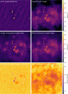 |
Fig. 2 Comparison of the reconstructions of the synthetic radio data using the single-component model (SCM) and the multi-component model (MCM, after the third iteration of aim-resolve). The first row shows the naturally weighted dirty image of the radio data and the underlying ground truth image. The following rows illustrate posterior mean and relative standard deviation of the reconstructions with the SCM and MCM after full convergence, respectively. The MCM reconstruction shows more precise and detailed reconstructions for the point sources and small extended objects, which is further illustrated by tighter flux contour lines around the sources in the MCM uncertainty map. |
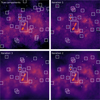 |
Fig. 3 Identified components for several iterations of aim-resolve applied to synthetic image data. Top left: ground truth along with the true components. Remaining panels: reconstructed posterior means for iterations 1-3, together with detected point sources (crosses) and extended objects (boxes), showing an increasing number of identified components and an enhancement in overall reconstruction quality across the iterations. |
4.2.2 Model comparison
When building the MCM, one still has to take care of how to set the priors for the hyper-parameters. For the point sources, we take the total flux from the previous reconstructed image with a wide standard deviation around it. For the correlation models, it is possible to set most of the hyper-parameters quite wide and flexibly, and just specify the overall offset depending on the previous reconstruction. An overview of the hyper-parameter priors for the different diffuse components is listed in Table B.1. We recall that the MCM is pre-fitted on the previous reconstruction and further optimized on the real data. This usually results in a full convergence of the model within a few major cycles, meaning that the reconstruction does not improve anymore.
Figure 2 shows the reconstructed posterior mean and relative uncertainties of both the MCM (after the third iteration of aim-resolve) and SCM along with the ground truth data. For a fair comparison, we further optimize the SCM after the first iteration of the method until full convergence. The MCM shows a better reconstruction of the diffuse background than the SCM. When looking at the point sources and small extended objects, the SCM shows some ringing effects around the sources. These nonphysical effects originate from the excitation of high-frequency modes in the power spectrum of the GP model. This enables the model to fit multiple compact sources, but introduces some ringing effects in the image. The MCM does not show this behavior as it describes compact objects by separate correlation models and point sources by a single pixel, which can be recognized by careful inspection of the MCM plot. Additionally, it captures more of the true components present in the data. A comparison of the relative uncertainties confirms that utilizing the MCM improves the description of the individual components and the diffuse background, but also the overall reconstruction of the data.
4.2.3 Component separation
In addition to the better reconstruction quality, the MCM efficiently separates point sources and extended objects from the background. Figure 4 illustrates the reconstructed posterior means of both the diffuse background and a combined plot of the point sources and extended objects of the MCM. All sources are well-separated from the background, which only shows the diffuse emission present in the data. We note that the MCM further enables us to get distinct plots for all individual model components.
4.3 Application to MeerKAT data
After validating the method on simulated data in the previous section, this section shows the application to a real MeerKAT observation. We applied aim-resolve to an L-band (856-1712 MHz) MeerKAT (Jonas & MeerKAT Team 2016) observation of the radio galaxy ESO 137-006. This dataset offers a great test case as it contains a combination of diffuse emission, point sources, and extended objects, notably the two radio galaxies ESO 137-006 and ESO 137-007.
The observation utilized all 64 MeerKAT antennas and the 4k mode of the SKARAB correlator in full polarization with 4096 channels for a total on target time of 14 hours. The novelty of this observation is the first discovery of collimated synchrotron threads connecting the two lobes of a radio galaxy, first presented by Ramatsoku et al. (2020). Since then, the data has been used by Dabbech et al. (2022) to demonstrate a sparsitybased imaging algorithm and Roth et al. (2024) to present the fast-resolve algorithm.
As in Ramatsoku et al. (2020), the data was averaged to 1024 frequency channels and divided into two sub-bands that are relatively free from radio frequency interference, the LO band (961–1145 MHz) and the HI band (1295–1503 MHz). These two sub-bands were phase self-calibrated using WSClean multi-scale CLEAN and CubiCal for imaging and calibration, respectively. For this work, we imaged only a subset of seven frequencies (986–1137 MHz) of the LO band with aim-resolve.
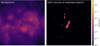 |
Fig. 4 Separate reconstructions of the components of the MCM in Fig. 2. Left: reconstructed posterior mean of the diffuse background. Right: combined plot of all point sources and extended objects. The sources are well separated from the background, which captures only the large-scale diffuse emission present in the data. |
4.3.1 Setup and identification
Similar to the synthetic case, we initialized the SCM with the wide hyper-parameter priors listed in Table B.1, but with a resolution of 1024 x 1024 and a FOV of 2° × 2°. Consequently, we chose the U-Net fine-tuned on the test-1024 data with the same resolution for the detection steps. As before we set a fixed minimal shape of 32 x 32 for the small extended object components to save computation time.
We ran aim-resolve for several iterations to continuously improve the overall reconstruction and component detection. Figure 5 shows the identified components in the second iteration of aim-resolve. The method detects the ESO 137-006 galaxy in the center of the FOV and the ESO 137-007 wide-tail galaxy above it, as well as most of the point sources and small extended objects. In summary, the U-Net detection still works for the MeerKAT wide-field radio observation allowing an efficient separation of the components in the following.
4.3.2 Reconstruction
As before, we set the priors for the MCM’s hyper-parameters similarly to Sect. 4.2.2, which can be found in Table B.1. We note that we needed the wide background FOV to capture all relevant sources present in the data. For plotting, however, we focused on the central 1° x 1° of the observation, which contains most of the flux. Figure 6 illustrates the resulting reconstructed posterior mean and relative standard deviation within this smaller FOV of the MCM fitted to the MeerKAT data (after the second iteration of aim-resolve). The reconstruction shows precise descriptions of the two foreground galaxies and of many small background sources. Moreover, the MCM captures fine structures such as the collimated synchrotron links of ESO 137-006, paired with a high certainty on these sharp structures.
The reconstruction features quite high background artifacts. They are also visible in the fast-resolve reconstructions from Roth et al. (2024). Since the sky prior models in resolve are flexible and therefore sensitive to miscalibrations in the data, this leads to imaging artifacts in the case of suboptimal calibration. Thanks to the multi-component approach, these artifacts are mainly absorbed into the background component, and therefore do not affect the reconstructions of the point sources and tile components.
4.3.3 Component separation
In addition to a good reconstruction quality, the MCM efficiently separates point sources and extended objects from the background. The first row of Fig. 7 illustrates the reconstructed posterior mean of both the background field and a combined plot of the point sources and small extended objects of the MCM. The second row depicts the two main galaxies ESO 137-006 and ESO 137-007. Because of the many sources present in the data and the suboptimal calibration, the method does not manage to separate all small sources from the background. Nevertheless, the background model has to describe considerably fewer sources than in the case of a SCM.
Finally, we emphasize that the application of aim-resolve to a large MeerKAT observation implies a trade-off between fidelity and runtime. Higher resolutions of the model would require either more GPU memory or the combination of several GPUs. The primary goal of this paper, however, is to showcase the applicability of the method to real data and not to reach the highest reconstruction fidelity.
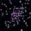 |
Fig. 5 Identified components in the second iteration of aim-resolve applied to the ESO 137-006 MeerKAT observation in the LO sub-band (961– 1145 MHz) with a FOV of 2° × 2°. The two large boxes indicate the identified galaxies ESO 137-006 and ESO 137-007. The remaining detected objects and point sources are marked with small boxes and crosses, respectively. |
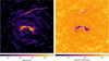 |
Fig. 6 Reconstruction of the ESO 137-006 MeerKAT observation in the LO sub-band (961–1145 MHz) using the MCM (after the second iteration of aim-resolve). The plots show 1° × 1° zoom-ins of the reconstructed posterior mean and relative standard deviation, covering the two foreground galaxies and many smaller sources. The relative uncertainty is lowest in high-brightness regions (indicated by the flux contours). |
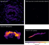 |
Fig. 7 Reconstructions of the individual components of the MCM in Fig. 6. The images show the reconstructed posterior mean of the background, of the sum of point sources and small extended components, and of the two galaxies ESO 137-006 and ESO 137-007. Most sources are well separated from the background, which captures only a few other objects in addition to the diffuse emission and calibration artifacts. |
5 Conclusions
In this work, we presented the method aim-resolve, designed to improve imaging for wide-field radio observations containing various different sources. We introduced the individual steps of the method, namely detection, modeling, separation and pre-fit, and reconstruction; and we combined them into an automatized and iterative method.
To validate the effectiveness of our method, we set up and solved a generic imaging problem. Within a few iterations, aim-resolve successfully identified all visible point sources and extended objects and efficiently separated them from the background. The utilization of different model descriptions allowed a more precise reconstruction of the individual components and improved the overall reconstruction of the data. Detailed plots of the reconstructed sky maps demonstrated the advantages of the multi-component approach.
In addition, aim-resolve was applied to an L-band (856– 1712 MHz) MeerKAT observation of the radio galaxy ESO 137006 and other radio galaxies in that environment. The method managed to identify and separate the two main galaxies ESO 137-006 and ESO 137-007 as well as many of the small extended objects and point sources. The multi-component reconstruction showed many details, especially in the fine structures of ESO 137-006, and a good description of small sources due to a clean separation of the modeled components.
The separation of the individual components could be used for detailed studies of interesting sources in that environment. Moreover, the gained knowledge on the identified components could be summarized to catalogs containing the positions, brightnesses, and other properties of point sources and extended objects in the FOV, together with the corresponding uncertainties. However, this is beyond the scope of this work.
A possible improvement of the method could be to allow a higher resolution of the components compared to the background. Furthermore, it would be beneficial to model the point sources directly in visibility space, making them completely independent from the underlying image resolution. While both enhancements are straightforward to set up with resolve, the current implementation of fast-resolve does not support them. While adding more highly resolved components leads to convolutions with very large kernels in the forward model, the explicit modeling of the point sources requires storing the full visibility data in GPU memory, which is infeasible for large datasets.
Another feature already implemented in resolve is unified imaging and calibration (Arras et al. 2019). Adding this feature to aim-resolve could help to remove a large fraction of the imaging artifacts present in the MeerKAT reconstruction. Moreover, it could be beneficial to combine the latent-space based point source detection of Guardiani et al. (2025) with the deep learning approach of aim-resolve.
Some interesting features of the ESO137-006 galaxy, for example the collimated synchrotron links, further motivate us to extend the multi-component sky model to handle multifrequency data and to model the spectral behavior of the different astrophysical components. This already has been done for other frequency bands and instruments using NIFTy (Scheel-Platz et al. 2023; Westerkamp et al. 2024; Eberle et al. 2026; Rüstig et al. 2024) and can give interesting insights into the evolution of radio-emitting plasmas in the imaged galaxies.
Finally, the full decoupling of the sky emission model and instrument response enables the application of aim-resolve to a wide variety of instruments and wavelength bands, just by an exchange of the response function paired with a slight adaption of the training dataset. This offers the stage for future multi-frequency and multi-instrument reconstructions.
Data availability
The raw data for the ESO137-006 observation is publicly available via the SARAO archive: https://archive.sarao.ac.za (project ID SCI-20190418-SM-01). The implementation of aim-resolve will be made publicly available on GitHub: https://github.com/rifu4/aim-resolve
Acknowledgements
R.F., V.E., and P.F. acknowledge funding through the German Federal Ministry of Education and Research for the project ErUM-IFT: Informationsfeldtheorie für Experimente an Großforschungsanlagen (Förderkennzeichen: 05D23EO1). L.H. and J.K. are supported by the Excellence Cluster ORIGINS, which is funded by the Deutsche Forschungsgemeinschaft (DFG, German Research Foundation) under Germany’s Excellence Strategy – EXC-2094-390783311. J.K. also acknowledges funding from the European Research Council (ERC) under the European Union’s Horizon 2020 research and innovation programme (ERC Synergy Grant “BlackHolistic”, Agreement No. 101071643). J.R. acknowledges financial support from the German Federal Ministry of Education and Research (BMBF) under grant 05A23WO1 (Verbundprojekt D-MeerKAT III). Funded by the European Union. Views and opinions expressed are however those of the author(s) only and do not necessarily reflect those of the European Union or the European Research Council Executive Agency. Neither the European Union nor the granting authority can be held responsible for them. This work is supported by ERC grant (mw-atlas, 101166905).
References
- Arras, P., Baltac, M., Ensslin, T. A., et al. 2019, Astrophysics Source Code Library [record ascl:1903.008] [Google Scholar]
- Arras, P., Frank, P., Leike, R., Westermann, R., & Enßlin, T. A. 2019, A&A, 627, A134 [NASA ADS] [CrossRef] [EDP Sciences] [Google Scholar]
- Arras, P., Bester, H. L., Perley, R. A., et al. 2021, A&A, 646, A84 [NASA ADS] [CrossRef] [EDP Sciences] [Google Scholar]
- Arras, P., Frank, P., Haim, P., et al. 2022, Nat. Astron., 6, 259 [NASA ADS] [CrossRef] [Google Scholar]
- Baldi, R., Capetti, A., & Massaro, F. 2018, A&A, 609, A1 [NASA ADS] [CrossRef] [EDP Sciences] [Google Scholar]
- Becker, R. H., White, R. L., & Helfand, D. J. 1995, ApJ, 450, 559 [Google Scholar]
- Bhatnagar, S., & Cornwell, T. J. 2004, A&A, 426, 747 [NASA ADS] [CrossRef] [EDP Sciences] [Google Scholar]
- Birdi, J., Repetti, A., & Wiaux, Y. 2019, MNRAS, 492, 3509 [Google Scholar]
- Blei, D. M., Kucukelbir, A., & McAuliffe, J. D. 2017, J. Am. Stat. Assoc., 112, 859 [CrossRef] [Google Scholar]
- Bowles, M., Scaife, A. M., Porter, F., Tang, H., & Bastien, D. J. 2021, MNRAS, 501, 4579 [CrossRef] [Google Scholar]
- Cai, X., Pereyra, M., & McEwen, J. D. 2018, MNRAS, 480, 4154 [Google Scholar]
- Capetti, A., Massaro, F., & Baldi. 2017a, A&A, 601, A81 [NASA ADS] [CrossRef] [EDP Sciences] [Google Scholar]
- Capetti, A., Massaro, F., & Baldi, R. D. 2017b, A&A, 598, A49 [NASA ADS] [CrossRef] [EDP Sciences] [Google Scholar]
- Cornwell, T. J. 2008, IEEE J. Sel. Top. Signal Process., 2, 793 [Google Scholar]
- Dabbech, A., Terris, M., Jackson, A., et al. 2022, ApJ, 939, L4 [NASA ADS] [CrossRef] [Google Scholar]
- Eberle, V., Guardiani, M., Westerkamp, M., et al. 2026, A&A, 706, A229 [NASA ADS] [CrossRef] [EDP Sciences] [Google Scholar]
- Edenhofer, G., Frank, P., Roth, J., et al. 2024, JOSS, 9, 6593 [Google Scholar]
- Ester, M., Kriegel, H.-P., Sander, J., & Xu, X. 1996, in Proceedings of the Second International Conference on Knowledge Discovery and Data Mining (KDD), 226 [Google Scholar]
- Frank, P., Leike, R., & Enßlin, T. A. 2021, Entropy, 23, 853 [NASA ADS] [CrossRef] [Google Scholar]
- Fuchs, R., Knollmüller, J., & Heinrich, L. 2025, Phys. Sci. Forum, 12, 15 [Google Scholar]
- Gendre, M., & Wall, J. 2008, MNRAS, 390, 819 [NASA ADS] [Google Scholar]
- Gendre, M., Best, P., & Wall, J. 2010, MNRAS, 404, 1719 [NASA ADS] [Google Scholar]
- Guardiani, M., Eberle, V., Westerkamp, M., et al. 2025, A&A, 703, A203 [NASA ADS] [CrossRef] [EDP Sciences] [Google Scholar]
- Högbom, J. 1974, A&AS, 15, 417 [Google Scholar]
- Hopkins, A. M., Whiting, M. T., Seymour, N., et al. 2015, PASA, 32, e037 [Google Scholar]
- Jonas, J., & MeerKAT Team 2016, MeerKAT science: on the pathway to the SKA, 1 [Google Scholar]
- Junklewitz, H., Bell, M., Selig, M., & Enßlin, T. 2016, A&A, 586, A76 [NASA ADS] [CrossRef] [EDP Sciences] [Google Scholar]
- Knollmüller, J., & Enßlin, T. A. 2018, arXiv preprint [arXiv:1812.04403] [Google Scholar]
- Lukic, V., de Gasperin, F., & Brüggen, M. 2019, Galaxies, 8, 3 [NASA ADS] [CrossRef] [Google Scholar]
- Miraghaei, H., & Best, P. 2017, MNRAS, 466, 4346 [Google Scholar]
- Mölder, F., Jablonski, K. P., Letcher, B., et al. 2021, F1000Research, 10 [Google Scholar]
- Offringa, A. R., & Smirnov, O. 2017, MNRAS, 471, 301 [Google Scholar]
- Proctor, D. 2011, ApJS, 194, 31 [Google Scholar]
- Ramatsoku, M., Murgia, M., Vacca, V., et al. 2020, A&A, 636, L1 [NASA ADS] [CrossRef] [EDP Sciences] [Google Scholar]
- Repetti, A., Pereyra, M., & Wiaux, Y. 2019, SIAM J. Imaging Sci., 12, 87 [Google Scholar]
- Ronneberger, O., Fischer, P., & Brox, T. 2015, in Medical Image Computing and Computer-assisted Intervention–MICCAI 2015: 18th International Conference, Munich, Germany, October 5–9, 2015, proceedings, part III 18 (Springer), 234 [Google Scholar]
- Roth, J., Arras, P., Reinecke, M., et al. 2023, A&A, 678, A177 [NASA ADS] [CrossRef] [EDP Sciences] [Google Scholar]
- Roth, J., Frank, P., Bester, H. L., et al. 2024, A&A, 690, A387 [NASA ADS] [CrossRef] [EDP Sciences] [Google Scholar]
- Rüstig, J., Guardiani, M., Roth, J., Frank, P., & Enßlin, T. 2024, A&A, 682, A146 [NASA ADS] [CrossRef] [EDP Sciences] [Google Scholar]
- Scheel-Platz, L. I., Knollmüller, J., Arras, P., et al. 2023, A&A, 680, A2 [NASA ADS] [CrossRef] [EDP Sciences] [Google Scholar]
- Schmidt, K., Geyer, F., Fröse, S., et al. 2022, A&A, 664, A134 [NASA ADS] [CrossRef] [EDP Sciences] [Google Scholar]
- Schwab, F. R., & Cotton, W. D. 1983, AJ, 88, 688 [Google Scholar]
- Selig, M., Bell, M. R., Junklewitz, H., et al. 2013, A&A, 554, A26 [NASA ADS] [CrossRef] [EDP Sciences] [Google Scholar]
- Taran, O., Bait, O., Dessauges-Zavadsky, M., et al. 2023, A&A, 674, A161 [NASA ADS] [CrossRef] [EDP Sciences] [Google Scholar]
- Terris, M., Dabbech, A., Tang, C., & Wiaux, Y. 2022, MNRAS, 518, 604 [NASA ADS] [CrossRef] [Google Scholar]
- Thompson, A. R., Moran, J. M., & Swenson, G. W. 2017, Interferometry and Synthesis in Radio Astronomy (Springer Nature) [Google Scholar]
- Thouvenin, P.-A., Abdulaziz, A., Dabbech, A., Repetti, A., & Wiaux, Y. 2022, MNRAS, 521, 1 [Google Scholar]
- Tiede, P. 2022, JOSS, 7, 4457 [Google Scholar]
- Tilley, D., Cleghorn, C. W., Thorat, K., & Deane, R. 2021, in 2021 IEEE Symposium Series on Computational Intelligence (SSCI), IEEE, 1 [Google Scholar]
- Vafaei Sadr, A., Vos, E. E., Bassett, B. A., et al. 2019, MNRAS, 484, 2793 [CrossRef] [Google Scholar]
- Wang, Z., Berman, M., Rannen-Triki, A., et al. 2023, in Advances in Neural Information Processing Systems, 36, eds. A. Oh, T. Naumann, A. Globerson, K. Saenko, M. Hardt, & S. Levine (Curran Associates, Inc.), 60144 [Google Scholar]
- Westerkamp, M., Eberle, V., Guardiani, M., et al. 2024, A&A, 684, A155 [NASA ADS] [CrossRef] [EDP Sciences] [Google Scholar]
- Wiaux, Y., Jacques, L., Puy, G., Scaife, A. M. M., & Vandergheynst, P. 2009, MNRAS, 395, 1733 [NASA ADS] [CrossRef] [Google Scholar]
Appendix A Transitions from the previous to the new sky model
The main idea of the transition model is outlined in Westerkamp et al. (2024) performing a switch from a single-frequency to a multi-frequency model. For our specific problem, we define a transition function that plausibly maps the parameters of the sky model of the previous aim-resolve iteration to the model parameters of the new iteration,
 (A.1)
(A.1)
Depending on the current iteration of aim-resolve, the previous model can be either a SCM or MCM whereas the new model usually has multiple components.
We implement the transition by stringing together multiple NIFTy inference problems. First, we create a mask around the predicted point sources and tile components of the new model and fit the masked background component of the new model to the previous reconstruction. With this step, we extract the predicted components from the background. For each predicted point source and tile, we fit a separate model component to the difference of the previous reconstruction and the newly optimized background. Finally, we put together the parameter vectors of the individual components and use this as a starting point for the next reconstruction step on the real data.
It should be noted that we omit any response function during the transition and perform the whole NIFTy optimization in image space. This corresponds to an identity response matrix in Eq. 1 and saves computation time.
Appendix B Prior parameters for the Gaussian process models
In Table B.1 we list the hyper-parameters (mean and standard deviation) of the Gaussian process model described in Sect. 3.1.2. They are similar for the SCM and the different components of the MCM, only the additional offset parameters of the models differ. For the SCM the offset is set to 12. For the MCM tile components it is set depending on the mean flux in the vicinity of the objects in the previous reconstruction. For the MCM background it is set to the mean flux of the whole reconstruction except the areas around detected components. We note that the remaining hyper-parameters are set quite wide to allow the model parameters to deviate sufficiently from the set prior values. The exact definitions of all model parameters are explained in detail in Arras et al. (2022).
Prior parameters for the Gaussian process models for the SCM and the MCM components.
Appendix C Additional plots
This section contains additional figures that were excluded from the main text to save space but that we nevertheless want to include for completeness. Figure C.1 depicts the natural weighted dirty image of the ESO137-006 MeerKAT observation. It serves as a starting point for the inference with aim-resolve.
Figure C.2 shows a subset of the train-128 data used to train the U-Net. The corresponding validation and test datasets contain similar images and labels but use distinct sets of galaxy-like objects from the RadioGalaxyDataset. The same holds for the datasets with resolutions of 512 X 512 and 1024 X 1024.
Figures C.3 and C.4 illustrate the reconstructed MCM posterior samples of the synthetic radio data and the ESO137-006 MeerKAT observation, respectively. These samples are used to build summary statistics of the approximate posterior distribution, for example the reconstructed posterior mean or the relative standard deviation that are shown in the applications section. The individual samples (e.g., in Fig. C.3) show differences especially in parts of the diffuse background, indicating high uncertainty in these areas. The opposite holds for the point sources and extended objects, resulting in low uncertainties at their locations.
 |
Fig. C.1 Natural weighted dirty image of the ESO137-006 MeerKAT observation in the LO sub-band (961 – 1145 MHz) in units of Jy/beam. |
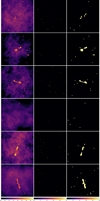 |
Fig. C.2 Subset containing six samples of the train-128 data used to train the U-Net. Each sample consists of an input image and two segmentation masks, one for point sources and one for extended objects (from left to right). |
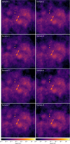 |
Fig. C.3 Reconstructed posterior samples of the synthetic radio data using the MCM (after the third iteration of aim-resolve). |
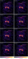 |
Fig. C.4 Reconstructed posterior samples (centrai 1° × 1°) of the ESO137-006 MeerKAT observation in the LO sub-band (961 – 1145 MHz) using the MCM (after the second iteration of aim-resolve). |
All Tables
Prior parameters for the Gaussian process models for the SCM and the MCM components.
All Figures
|
Fig. 1 Visualization of the iterative method of aim-resolve. Initialized with a single-component model (0), it generates a preliminary reconstruction of the data (d). It detects point sources and extended objects in the reconstruction (a) and adds the identified components, marked with crosses and boxes, to the existing background model (b). Next, it separates the components from the background and fits them to the previous reconstructed image (c), before it continues the optimization on the real data (d). This cycle is repeated multiple times for further refinement. |
| In the text | |
|
Fig. 2 Comparison of the reconstructions of the synthetic radio data using the single-component model (SCM) and the multi-component model (MCM, after the third iteration of aim-resolve). The first row shows the naturally weighted dirty image of the radio data and the underlying ground truth image. The following rows illustrate posterior mean and relative standard deviation of the reconstructions with the SCM and MCM after full convergence, respectively. The MCM reconstruction shows more precise and detailed reconstructions for the point sources and small extended objects, which is further illustrated by tighter flux contour lines around the sources in the MCM uncertainty map. |
| In the text | |
|
Fig. 3 Identified components for several iterations of aim-resolve applied to synthetic image data. Top left: ground truth along with the true components. Remaining panels: reconstructed posterior means for iterations 1-3, together with detected point sources (crosses) and extended objects (boxes), showing an increasing number of identified components and an enhancement in overall reconstruction quality across the iterations. |
| In the text | |
|
Fig. 4 Separate reconstructions of the components of the MCM in Fig. 2. Left: reconstructed posterior mean of the diffuse background. Right: combined plot of all point sources and extended objects. The sources are well separated from the background, which captures only the large-scale diffuse emission present in the data. |
| In the text | |
|
Fig. 5 Identified components in the second iteration of aim-resolve applied to the ESO 137-006 MeerKAT observation in the LO sub-band (961– 1145 MHz) with a FOV of 2° × 2°. The two large boxes indicate the identified galaxies ESO 137-006 and ESO 137-007. The remaining detected objects and point sources are marked with small boxes and crosses, respectively. |
| In the text | |
|
Fig. 6 Reconstruction of the ESO 137-006 MeerKAT observation in the LO sub-band (961–1145 MHz) using the MCM (after the second iteration of aim-resolve). The plots show 1° × 1° zoom-ins of the reconstructed posterior mean and relative standard deviation, covering the two foreground galaxies and many smaller sources. The relative uncertainty is lowest in high-brightness regions (indicated by the flux contours). |
| In the text | |
|
Fig. 7 Reconstructions of the individual components of the MCM in Fig. 6. The images show the reconstructed posterior mean of the background, of the sum of point sources and small extended components, and of the two galaxies ESO 137-006 and ESO 137-007. Most sources are well separated from the background, which captures only a few other objects in addition to the diffuse emission and calibration artifacts. |
| In the text | |
|
Fig. C.1 Natural weighted dirty image of the ESO137-006 MeerKAT observation in the LO sub-band (961 – 1145 MHz) in units of Jy/beam. |
| In the text | |
|
Fig. C.2 Subset containing six samples of the train-128 data used to train the U-Net. Each sample consists of an input image and two segmentation masks, one for point sources and one for extended objects (from left to right). |
| In the text | |
|
Fig. C.3 Reconstructed posterior samples of the synthetic radio data using the MCM (after the third iteration of aim-resolve). |
| In the text | |
|
Fig. C.4 Reconstructed posterior samples (centrai 1° × 1°) of the ESO137-006 MeerKAT observation in the LO sub-band (961 – 1145 MHz) using the MCM (after the second iteration of aim-resolve). |
| In the text | |
Current usage metrics show cumulative count of Article Views (full-text article views including HTML views, PDF and ePub downloads, according to the available data) and Abstracts Views on Vision4Press platform.
Data correspond to usage on the plateform after 2015. The current usage metrics is available 48-96 hours after online publication and is updated daily on week days.
Initial download of the metrics may take a while.