


| Issue |
A&A
Volume 711, July 2026
|
|
|---|---|---|
| Article Number | A123 | |
| Number of page(s) | 15 | |
| Section | Astrophysical processes | |
| DOI | https://doi.org/10.1051/0004-6361/202557467 | |
| Published online | 06 July 2026 | |
Microlensing timescales and flux magnification probabilities of a sample of 204 lensed quasars
1
Instituto de Física y Astronomía, Facultad de Ciencias, Universidad de Valparaíso, Av. Gran Bretaña 1111 Valparaíso, Chile
2
Instituto de Astrofísica de Canarias, Vía Láctea S/N, La Laguna, 38200, Tenerife, Spain
3
Departamento de Astrofísica, Universidad de la Laguna, La Laguna, 38200, Tenerife, Spain
★ Corresponding authors: This email address is being protected from spambots. You need JavaScript enabled to view it.
; This email address is being protected from spambots. You need JavaScript enabled to view it.
Received:
29
September
2025
Accepted:
4
May
2026
Abstract
Context. Quasar microlensing is a very useful tool in cosmology and astrophysics, as well as a source of uncertainty in certain investigations, such as the determination of the Hubble constant from lensed quasars. Microlensing probability and timescales have been studied statistically using the Einstein ring crossing time of an isolated mass as a reference scale.
Aims. Our goal is to extend the statistical analysis of microlensing to all currently known lensed quasars with the data currently available, while considering realistic optical depths and the gravitational effect of the lens galaxy. We take into account new observational results on quasar sizes and the peculiar velocities of lens galaxies.
Methods. We applied automatic lens modeling to the 204 systems available. For each image, we computed microlensing magnification maps and histograms.
Results. Using thin disk source sizes scaled to take into account recent measurements of accretion disk sizes, we find a mean source crossing time of 2.59 ± 0.07 years. The mean Einstein radius crossing time is 11.29 ± 0.05 years. When a fraction of mass in microlenses α = 0.2 is adopted, we find a good matching between the modeled histogram of mean microlensing magnifications for the images in our sample and the experimental histogram of microlensing magnifications.
Conclusions. From the modeling of microlensing magnification histograms, we estimated the average half-light radius of the quasar source, R1/2 = 5.4 ± 2.7 light-days, and a lower limit to the mass fraction in microlenses, α ≥ 0.15. From the microlensing magnification maps, we find that a lensed quasar image has a mean probability of approximately 9% of being involved in a high-magnification event (Δm ≤ −0.32). We selected a group of images with the highest probabilities and the smallest crossing times.
Key words: gravitational lensing: strong / gravitational lensing: weak / quasars: general
© The Authors 2026
 Open Access article, published by EDP Sciences, under the terms of the Creative Commons Attribution License (https://creativecommons.org/licenses/by/4.0), which permits unrestricted use, distribution, and reproduction in any medium, provided the original work is properly cited.
This article is published in open access under the Subscribe to Open model. This email address is being protected from spambots. You need JavaScript enabled to view it. to support open access publication.
1. Introduction
The discovery of the first gravitationally lensed quasar in 1979 by Walsh et al. (1979) opened up a new field of study that had previously existed only in theory. Nearly 45 years have passed since then and the number of known systems has reached more than 300 (Muñoz et al. 1998; Treu et al. 2018; Lemon et al. 2018; Chan et al. 2024). This number is continually growing with projections for about 10 000 more in the coming years (Oguri & Marshall 2010; Collett 2015; Ivezić et al. 2019).
Multiply imaged quasars provide valuable insights into the mass distribution, formation, and evolution of lens galaxies, either disk or elliptical galaxies, the most common type of lens (Treu 2010). They also help to constrain the stellar initial mass function (IMF) and to measure various cosmological parameters (see Jiménez-Vicente & Mediavilla 2019; Shajib et al. 2024, for recent reviews). In particular, a notable capability of gravitationally lensed quasars is their potential to determine the Hubble constant (H0). Incorporating this method into the current suite of measurements may help to resolve the persistent 5σ tension in the inferred value of the Hubble constant (Tully 2023; Di Valentino et al. 2021; Verde et al. 2024).
In general, the macrolens responsible for producing multiple images of a quasar is well described by the smooth gravitational potential of the lens galaxy. However, real galaxies are granular: stars (and possibly other compact objects) introduce small-scale perturbations to the potential that differentially magnify distinct quasar-emitting regions. This effect is called gravitational microlensing and produces time- and wavelength-dependent variations in the image flux ratios (e.g., Refsdal & Stabell 1997; Wambsganss 2006; Vernardos et al. 2024). Quasar microlensing is therefore a powerful probe of quasar structure across a wide range of spatial scales from the immediate vicinity of the Supermassive black hole (SMBH) event horizon (Morgan et al. 2010), to the accretion disk (Cornachione & Morgan 2020; Fian et al. 2021), the broad line region (BLR; Abajas et al. 2002; Hutsemékers et al. 2024), and the dusty torus (Sluse et al. 2013). At the same time, microlensing statistics constrain the fraction of mass in compact objects and can be used to test lens-galaxy stellar mass functions (e.g., present-day mass function over the IMF) and the abundance of potential dark matter candidates (e.g., Wyithe & Turner 2001; Jiménez-Vicente & Mediavilla 2019; Esteban-Gutiérrez et al. 2023; Awad et al. 2023).
The advent of wide-field time-domain surveys, most notably the Vera C. Rubin Observatory Legacy Survey of Space and Time (LSST; Ivezić et al. 2019), will deliver multi-band monitoring for large samples of lensed quasars and will make it feasible to systematically study high-magnification events (HMEs). These phenomena are typically defined as sharp, transient brightenings caused by the source approaching or crossing a micro-caustic, and they can provide especially strong constraints on the source size and surface-brightness profile because the caustic effectively “scans” the emitting region (Anguita et al. 2008; Mediavilla et al. 2015). In this context, dedicated forward-modeling tools tailored to LSST cadences have been developed (Neira et al. 2020) and recent simulations predict that an order of ∼60 HMEs per year (with amplitudes > 0.3 mag in r) could be detectable based on simulated ∼4 billion light curves (Neira et al. 2025). These forecasts motivate early-warning and triggering strategies for dense follow-up during HMEs when the information content for quasar-structure inference is maximal (e.g., Fagin et al. 2024).
Consequently, the study of microlensing properties of known lensed quasars, in particular, its timescale-flux variations, is a key ingredient for the analysis of future systems. Early studies (see, e.g., Kochanek 2004; Wambsganss 2006) indicate that the microlensing timescale is between months and years. In an extensive analysis Mosquera & Kochanek (2011, hereafter M&K) developed a procedure to estimate this timescale for the 87 known systems at that time, with timescales ranging from months to decades. M&K based their analysis on the Einstein radius (θE) crossing time, a quantity defined for a single, isolated lens, which does not take into account the cooperative effects between microlenses corresponding to the relatively large optical depths typical of lensed quasars and the external gravitational field of the lens galaxy.
For compact microlenses, microlensing magnification patterns are scaled to the Einstein radius of the microlenses in the sense that if we, for instance, change the mass of the microlenses, M → M′, all the lengths should be rescaled by a  factor (mass-length invariance, Wambsganss 2006). However, apart from this global change of scale, the Einstein radius crossing time may not be informative about the timescales of flux variations or about any pseudo-periodical properties of quasar microlensing (Wyithe & Turner 2002). The frequency of variations is dominated by the optical depth of the microlenses and the shear of the macroscopic gravitational field of the lens galaxy (Paczynski 1986; Gil-Merino & Lewis 2005). On the one hand, even at low optical depth, closed caustic curves (the typical astroids) are magnified by the effect of the shear. On the other hand, as the optical depth increases, single closed caustic curves can progressively interconnect forming first constellations and then intricate networks with high spatial frequencies (compensated by large demagnification regions). None of these effects are directly related to the Einstein radius crossing time for an isolated particle Schneider et al. (1992). The way to obtain more information about the properties of microlensing variability is, then, to simulate microlensing for the particular conditions of the gravitational field at each lensed quasar image. Microlensing magnification maps are the usual tool applied in this type of study (Kayser et al. 1986).
As mentioned before, nearly fifteen years have passed since the work by M&K and the number of known lensed quasar systems has almost quadrupled (Chan et al. 2024). Moreover, new information about the size of the quasar accretion disk and about the lens galaxy peculiar velocities, both critical to study the microlensing timescales, are now available. Specifically, microlensing (Jiménez-Vicente et al. 2012; Cornachione & Morgan 2020) and reverberation mapping measurements (Fausnaugh et al. 2018; Jha et al. 2022) indicate that the accretion disk size is several times larger than the estimates based on the thin disk model by (Shakura & Sunyaev 1973, hereafter, S&S). Taking this effect into account, we rescale the theoretical size previously used in M&K using microlensing estimations.
On the other hand, in addition to the calculations based on Einstein ring crossing times and to take into account realistic values of the optical depth of lensed quasar images, we calculated magnification maps for every image, which also informs us about the relative probability (and timescales) of different levels of microlensing activity. To compute the statistically significant magnification probabilities, we chose to use fast multipole method–inverse polygon mapping (FMM–IPM; Jiménez-Vicente & Mediavilla 2022), which makes it possible to calculate large enough microlensing magnification maps for a large number of lensed images. As mentioned above, the amplitude of microlensing flux magnification is another important property that we analyzed from these magnification maps.
As a first step in this study, we performed homogeneous and simple parametric automatic modeling for all the gravitational lens quasars to avoid systematics associated with the lens modeling process. Consequently, we also obtain a complete sample of lens model parameters useful to analyze the properties of the population of lensed quasars systems.
The paper is organized as follows. Section 2 presents our dataset. Section 3 describes the macro-modeling procedure, the computation of magnification maps, and the calculation of relevant timescales and probabilities. Results are presented in Sect. 4 and discussed in Sect. 5. Finally, the main conclusions are summarized in Sect. 6. Throughout this paper, we adopt the following cosmological parameters: Ωm = 0.3, Ωm = 0.7, and H0 = 70 km/s/Mpc.
2. Data
The first uniform and high-resolution image database of gravitationally lensed quasars was provided in the 1990s by the CfA–Arizona Space Telescope LEns Survey1 (CASTLES; Muñoz et al. 1998). Using the Hubble Space Telescope (HST), broad-band images were obtained for ∼100 systems, primarily in the filters F160W, F814W, and F555W, including 15 galaxy-scale quadruply lensed quasars.
Decades later, in 2015, the Strong Lensing Insights into the Dark Energy Survey (STRIDES; Treu et al. 2018) initiated a new search for lensed quasars in the Dark Energy Survey The Dark Energy Survey Collaboration (2005), aiming to discover new quadruply lensed quasars and to select the best candidates for a time-delay follow-up and H0 estimation. The initial search was subsequently expanded to incorporate Gaia data (Krone-Martins et al. 2018), which enabled the exclusion of stars as contaminants (Lemon et al. 2017; Agnello et al. 2018; Lemon et al. 2023).
A few years ago, the Gravitationally Lensed Quasar Database (GLQD) listed the names and references of most known lensed quasars. However, the information provided for the systems was not homogeneous, and the page has since been taken down. New projects, such as the Strong Lensing Database (SLED2), have emerged to fill this gap, aiming to provide a unified and comprehensive database of strong lensing systems. However, it still does not provide complete information (e.g., photometry in multiple bands for the images) for all the known systems.
Considering this inhomogeneity, we construct a dataset to identify the largest collection of systems containing photometric information for the images, relative astrometry, and the redshifts of both the lens and source. To achieve this, we began our search with the systems published in the CASTLES database, where objects are reported with their photometric data in the HST bands, relative astrometry, and redshift information for the source and lens. Next, we turned to the GLQD and search the literature for photometric and relative astrometric data on the latest discovered systems. We also included systems not listed in either of the databases above. Since the redshift estimates for the source and lens are not always reported in the same publication, we searched for the most recent publicly available values. Our search produced an output sample of 314 known systems, each with different levels of information. This census can be accessed online3.
In this paper, we also compare our estimates of microlensing magnification probabilities with the observed microlensing histogram presented by Mediavilla et al. (2009, hereafter MED09; see also Mediavilla et al. 2024). This empirical histogram is constructed from single-epoch microlensing measurements of image pairs and, therefore, it does not preserve the sign of the magnification. For this reason, we also computed the probability distributions for the unsigned value of the microlensing magnification.
3. Methods
3.1. Macro lens modeling
Over the last decades, different lens modeling software (Lefor et al. 2013) with a variety of approaches have been applied to study individual systems (Shajib et al. 2022), meanwhile, the use of machine learning techniques is starting to appear to tackle the upcoming thousands of objects that will be discovered (Andika et al. 2025; Erickson et al. 2025). For example, to model complex systems using high-resolution images (i.e., quadruply lensed quasars with extended arcs), several codes exist, in particular the two well-tested modeling codes Lenstronomy (Birrer et al. 2015; Birrer & Amara 2018) and Glee (Gravitational Lens Efficient Explorer; Suyu et al. 2010). Both codes were used in auto-modeling task (see Schmidt et al. 2023; Ertl et al. 2023), concluding that for some of the systems, human supervision is still required. In fact, a few of the modeling codes offer a native automatic process. One example is AutoLens (Nightingale et al. 2021). This code uses a non-linear search to determine the set of light and mass profile parameters that best fit the data using images of the objects (see more details in pyautolens docs4).
Another difficulty is that the kind of observational data required by the most complex codes (e.g., line-of-sight velocity dispersion, high-resolution images Knabel et al. 2025) are not available for a significant part of the known quasar lenses.
As our aim here has been to study as many systems as possible using a homogeneous procedure, we adopted a straightforward approach based solely on photometric data from the lensed quasar images and on the relative positions between the images and the lens galaxy, which are typically available in the literature. We selected Lensmodel (Keeton 2001b, 2011), a parametric gravitational lens modeling code that the community has extensively tested for over two decades. This code supports a wide range of analytic mass distributions and can fit lens systems using constraints from image positions and flux ratios. The modeling can be performed either in the image plane or in the source plane. In our case, we adopted the image-plane approach, in which the code minimizes a standard chi-square statistic of the form,
 (1)
(1)
where θi, mod and θi, obs are the modeled and observed image positions (in arcseconds) respectively, with positional uncertainties, σi, θ. In addition, fi, mod and fi, obs are the modeled and observed fluxes with flux uncertainties, σi, f. The goal is to determine the set of lens model parameters that minimizes χ2, thereby yielding the best match between the model predictions and the observational constraints.
Building on this well-established code, we developed quasar microlensing analysis (QuMAS)5. It is a Python wrapper that implements an automatic modeling pipeline and the methodologies presented in this work. This framework enables fully automated lens modeling, allowing us to systematically analyze a large number of systems with a consistent methodology. Below, we detail the steps of this automatic pipeline. In Sect. 4.1.2, we compare our results with those from more complex or sophisticated models to assess how much a single model that captures the essence of the phenomenon, can differ from a more elaborated one. Next, we explain our automatic modeling procedure and its application to our current data sample. The steps of the procedure as as follows.
We start by modeling the 314 systems using the most recent and accurate photometry and astrometry available in the I band (λ = 8140 Å) or similar. The first filter checks whether the system contains known relative astrometry and photometry for all images, which results in a sample of 204 systems that can be modeled. The initial model applied is a singular isothermal sphere (SIS, Keeton 2001a), the simplest mass distribution and a common first approximation in many cases. The initial conditions for image uncertainties are derived from the data census. The galaxy position uncertainty is fixed at 10−3 arcseconds, providing a strong constraint, and the fluxes are also taken from the census with an associated error of 20%. This uncertainty in the fluxes accounts for the effects of microlensing in one or more images, which can introduce additional magnification. The value is chosen as a conservative estimate based on the literature (Morgan et al. 2010; Vives-Arias et al. 2016; Morgan et al. 2018), where the reported uncertainties range between 10% and 50%.
To evaluate the convergence of the model, in addition to a χ2 value, we also assess the agreement between the model and the data by computing the maximum separation between the calculated and the observed image positions(Δθmax), defined as
 (2)
(2)
 (3)
(3)
 (4)
(4)
This choice was motivated by the potential uncertainties associated with flux measurements and our threshold for determining the quality of the modeling. We consider a model successful if Δθmax ≤ 10−2 arcseconds. This threshold is based on the error distribution of the census images (Fig. 1). Although the specific median positional error was 10−3 arcseconds, we adopted a threshold five times larger to allow for a simpler model.
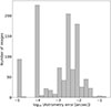 |
Fig. 1. Astrometric error distribution for the sample of images modeled. |
If the model is successful, we take the values of the convergence (κ), which represents the dimensionless surface mass density of the lens; the shear (γ), which is associated with the distortion induced by the tidal gravitational field of the lens and its environment, along with the Einstein radius, given its proportionality to the lens galaxy mass, as provided by Lensmodel. We then estimate the uncertainties using the Markov chain Monte Carlo (MCMC) method implemented in Lensmodel. The MCMC is initialized using the modeling parameters as Gaussian priors, and is run with ten chains and a maximum of 10 000 steps.
If the condition (Δθmax ≤ 10−2 arcseconds) is not satisfied, the system will be remodeled based on the number of images. For doubles, we consider models such as singular isothermal ellipsoid (SIE, Kormann et al. 1994), or SIS with γ, where shear represents an external gravitational perturbation introducing ellipticity. For quads, the modeling options expand to include SIE, SIS+γ, power-law mass distributions (POW, Keeton 2001a), SIE+γ, or POW+γ. The larger number of images in quads allows for testing a greater variety of mass distributions due to the increased number of free parameters.
If the system cannot be successfully modeled, we return to step 3 and modify the initial conditions. We first increase the images flux error to 50%, keeping the lens galaxy position error unchanged. Next, we set the flux error to 20% and increase the lens galaxy position error to 0.1 arcseconds. These changes help address scenarios where external shear effects are insufficient to characterize distortions and the centroid of the potential does not coincide with the center of the light distribution of the lens galaxy. Finally, we run a model with a flux error of 50% and a lens galaxy position error of 0.1 arcseconds. If no modeling option succeeds after all these attempts, to preserve the maximum number of systems in the sample, we end up selecting the model with the smallest Δθmax and Lensmodelχ2.
3.2. Microlensing timescales
The relative motion between the observer, lens, and source results in the time-dependent microlensing effect. Two temporal scales can be associated with microlensing (for a recent review see Sect. 3.5.6 of Vernardos et al. 2024). One is the basic temporal scale standard, tE, which is defined as the time it takes for the source to cross the Einstein radius of a single, isolated microlens (RE) and can be written as
 (5)
(5)
where v corresponds to the effective velocity of the source, and RE is, defined as
![Mathematical equation: $$ \begin{aligned} R_E=D_{OS}\left[ \frac{4G M_{\star }}{c^2}\frac{D_{LS}}{D_{OL}D_{OS}}\right]^{1/2}, \end{aligned} $$](/articles/aa/full_html/2026/07/aa57467-25/aa57467-25-eq7.gif) (6)
(6)
where DOS, DLS, and DOL correspond to the angular diameter distances between obs-source, lens-source, obs-lens, G is the gravitational constant, c is the speed of light, and M★ corresponds to the mass of the star acting as a microlens. To calculate RE, we assume a value of M★ = 0.3 M⊙. Two reasons drive this assumption: (1) this is the value estimated by Holtzman et al. (1998) observing the Baade’s window in the Galactic bulge using Hubble space telescope; and (2) this value has been used largely in previous microlensing studies (see Mao 2012; Jiménez-Vicente et al. 2014; Fian et al. 2018; Paic et al. 2022).
According to M&K, the tE timescale is expected to be on the order of decades (see Smith et al. 2009; Bonaca et al. 2017). However, if the source crosses a compact region of very high magnification such as one of the caustic curves (Blandford & Narayan 1992) shown in Fig. 2, it is possible to observe microlensing variations in shorter timescales; this timescale is known as the crossing timescale, tS, and defined as
 (7)
(7)
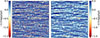 |
Fig. 2. Microlensing magnification patterns produced by stars in the lensing galaxy corresponding to image A of the system DES2158−5812. Left: Original magnification map. The color scale encodes different magnification levels, while the diamond-shaped curves trace the caustics. Right: Same map after convolution with a Gaussian profile with a sigma size of 3.72 [pix], showing the effective magnification pattern. Both panels have a size of 1200 × 1200 pixels with a pixel size of 1.1 [pix/light-days] and 60 RE. The maps were produced using the code developed in Jiménez-Vicente & Mediavilla (2022). |
Here, RS represents the radius of the light source, and it can be estimated assuming a simple thin-disk model (Shakura & Sunyaev 1973), with a temperature profile of T ∝ R−3/4 thus (M&K),
 (8)
(8)
where i is the average inclination of the quasar disk, zpt is the zero point, which depends on the photometric system and broad band used, λ is the reference wavelength corresponding to the mean of the band in which the observations were made, and m is the source aparent magnitude after removing the gravitational lens magnification (i.e., demagnified magnitude). The values for zpt and λ are not always available in the literature, so we obtained them from the Filter Profile Service (Rodrigo & Solano 2020)6 using the specified instrument and band. For objects where this information is not explicitly provided, we assumed a Vega system zpt.
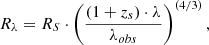
Following other authors, we adopt i = π/3, which corresponds to the average inclination of known systems (see Wildy & Czerny 2017). Since not all systems have observations at the same wavelength (λobs), we rescaled all the obtained RS using the thin-disk model approximation, Rλ ∝ λ4/3, to a reference rest-frame wavelength of λ = 0.250 μm. Following Morgan et al. (2010), we use the equation,
 (9)
(9)
where Rλ corresponds to the size of the radius at the rest-frame, λ, and RS is the radius obtained from Eq. (8), with λobs as the wavelength of the observed band.
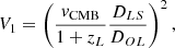
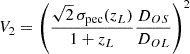
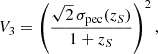
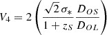
Next, we introduce the velocity model used to estimate the scales (see Eqs. 5 and 7), also known as the effective velocity of the source (v). This is calculated considering the relative motions of observer, lens, and source (Kayser et al. 1986), using Eq. 8 from Mediavilla et al. (2016):
 (10)
(10)
Hence, we have
 (11a)
(11a)
 (11b)
(11b)
 (11c)
(11c)
 (11d)
(11d)
In Eq. (11a), vCMB represents the projection of the CMB dipole velocity. This velocity depends on both the velocity and coordinates of the CMB, as well as the coordinates of the object. It is calculated following Poindexter & Kochanek (2010), assuming a velocity of CMB of 369.82 ± 0.11 km/s at right ascension and declination coordinates, respectively, of RA 167° .942 ± 0° .007 and DEC −6° .944 ± 0° .007 (Planck Collaboration I 2020).
The peculiar velocity (σpec) in Eqs. (11b) and (11c) refers to the velocity at which a galaxy deviates from the Hubble flow at a given redshift. We can estimate this by following the steps of Mediavilla et al. (2016), assuming the linear regime in a ΛCDM cosmology. In this framework, σpec can be expressed in terms of the cosmological growth rate factor f(z) as
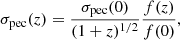 (12)
(12)
adopting the peculiar velocity at redshift zero from Heß & Kitaura (2016)σpec(0) = 439 ± 69 km s−1. Then, f(z) can be calculated using
 (13)
(13)
where Ωm(z) is the matter density parameter and γ is the growth index, with γ = 0.55 for the lambda cold dark matter cosmology (ΛCDM; (Avila et al. 2022)).
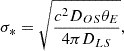
Finally, σ* in Eq. (11c) represents the velocity dispersion of the stars in the lens galaxy. It is estimated using the SIE mass distribution, following previous works (Grillo et al. 2008; Treu et al. 2009) and expressed as
 (14)
(14)
In those cases where the lens or source redshift is unknown, we follow Coe & Moustakas (2009), Redlich et al. (2012), Robertson et al. (2020) and similar works, where they are typically assumed to be zL ∼ 0.5 and zS ∼ 2.0, respectively. This assumption allows us to be consistent with previous works and the distribution of redshift in our sample (e.g., Treu et al. 2018; Schmidt et al. 2023)
3.3. Microlensing magnification maps
The Einstein radius defined in the previous section applies to a single, isolated microlens. However, the microlensing of lensed quasar images is associated with a relatively high optical depth of the microlenses, and cooperative effects between them are expected. To estimate the probability and timescales of microlensing in this scenario, we chose to use microlensing magnification maps. The probability density functions (PDFs) of microlensing magnification obtained from these maps provide information about the probability of brightness anomalies with respect to the intrinsic flux-ratios between images.
The analysis of magnification maps is a vital component of microlensing studies. In recent years, developments in this field have advanced significantly, particularly through the incorporation of GPU-based methods (e.g., Weisenbach 2025) and large public databases such as GERLUMPH (Vernardos et al. 2014, 2015), which contain thousands of high-resolution magnification maps, as well as through updates to classical techniques, such as the FMM–IPM Jiménez-Vicente & Mediavilla (2022), an improved version of the classical inverse polygon mapping method (Mediavilla et al. 2006, 2011). In this study, we employ the FMM–IPM, which has been used extensively in microlensing analyses (e.g., Jiménez-Vicente & Mediavilla 2025; Fian et al. 2024; Esteban-Gutiérrez et al. 2023), and whose magnification maps can be queried online7.
The parameters used to generate the magnification maps include the convergence, κ, and shear, γ, obtained from the lens modeling (their distributions are shown in Fig. 4); the fraction of the total convergence in microlenses, defined as α = κ*/κtot; and the microlens Einstein radius (see Eq. (6)). The magnification maps have a physical size of 60 Einstein radii, with pixel dimensions ranging from 400 (Q2237+030) to 3800 (WISE2329-1258), corresponding to an average scale of approximately 1.1 light-days per pixel. This resolution is sufficient to avoid introducing additional biases in our results, as demonstrated by Vernardos & Fluke (2013).
Magnification maps are generated for two values of α. We select α = 0.1 and α = 0.2, taking into consideration a low stellar mass fraction that has been reported in some microlensing studies, with values of around a few percent to 10% (Mediavilla et al. 2009), consistent with the notion that lens galaxies are largely dominated by dark matter at the radius of the quasar images. Then, in more recent analyses that include finite-source effects and larger samples, higher stellar mass fractions are indicated, converging on α ∼ 0.2 as a representative value near the Einstein radius (Jiménez-Vicente et al. 2015). This result is also in line with strong-lensing and dynamical studies of early-type lens galaxies, which suggest that stars contribute roughly 10–30% of the surface mass density at a few effective radii (e.g., Vernardos et al. 2024). Thus, by adopting α = 0.1 and 0.2, we were able to bracket the most plausible range of stellar mass fractions inferred for lensing galaxies, while also ensuring comparability with previous microlensing studies that commonly use these values as benchmarks. One example of such a magnification map is shown in Fig. 2.
To account for the magnification of a finite-size source, maps were convolved with a Gaussian source profile of standard deviation rs, I(r)∝exp( − r2/2rs2). As shown by Mortonson et al. (2005), the specific shape of the brightness profile does not strongly affect the statistical magnification properties, but just its half-light radius, which for a Gaussian profile is R1/2 = 1.18rs and R1/2 = 2.44RS (i.e., rs = 2.07RS). The rs values for each system are inferred from thin-disk estimates of RS, rescaled to the median size derived from microlensing observations (see Sect. 4.2).
For each system image, magnification maps are generated using the corresponding κ and γ values. The physical size of the maps varies among systems to preserve a fixed pixel resolution in light-days. We consider two values of the microlensing mass fraction, α = 0.1 and 0.2, and three source-size scalings, 0.3 × rs, 1 × rs, and 2 × rs. For each set of (α, rs), this yields 520 magnification maps for the full sample consisting of 149 doubles, 53 quads, and 2 five-image systems. This gives a total of 3120 convolved maps for all the pairs (α, rs). These maps can be used to study the effects of α and rs on the magnification probability distributions and combined with observational microlensing constraints, they allow us to evaluate the likelihood of different parameter combinations (Sect. 4.3).
4. Results
4.1. Homogeneous estimate of the Einstein radius
The homogeneous modeling of gravitational lensing systems provides an estimate of the parameters that define our model. The Einstein radius is the most relevant for our study, given its proportionality with the lens galaxy mass. To ascertain the robustness of our estimations, we compare them with those obtained in the literature and with other codes.
4.1.1. Comparison with previous studies not based on automatic modeling
To make a comparison with the literature, we use the sample of lensed quasars selected by Amante et al. 2020, which compiles the θE values individually obtained for each system (see Fig. 3). The agreement is, in general, excellent, except for two systems. One of them, SDSS1155+6346 (Pindor et al. 2004), is a double lens quasar, and the model selected in the literature was chosen from Rojas et al. (2014). In their work, they selected a SIS+γ model while our model is an SIE for this system. The discrepancy might be related to the difference in mass distribution selection. The other case is HS0818+1227 (Hagen & Reimers 2000). This system is a double and the model selected, as cited in Leier et al. (2011), is affected by a close external galaxy, which impacts the estimation of the Einstein radius.
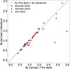 |
Fig. 3. Comparison of θE in this work vs. values in the literature for modeled lens quasars. The systems that are clearly far from a 1:1 relation are SDSS 1155+6346 and HS 0818+1227. |
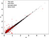 |
Fig. 4. Values of κ and γ for our sample (red filled diamonds), compared with literature samples: unfilled black diamonds Neira et al. (2025), unfilled circles Ertl et al. (2023), and unfilled black squares Schmidt et al. (2023). |
4.1.2. Comparison with previous automatic modeling studies
The newest discovered quadruple systems have been automatically modeled using HST high-resolution images. Schmidt et al. (2023) shows the results for thirty quadruply lensed quasars obtained with LENSTRONOMY. We modeled 29 of the 30. The missing model system corresponds to J1721+8842, the first confirmed ZigZag lens (Dux et al. 2025), consisting of two lens galaxies at different redshifts. For the remaining 29, we obtained a good agreement for 27, with a difference in the RE < 0.01 arcsec (see Fig. 3). The other two systems are J0343-2828 (Lemon in prep., which has a fifth image) and 2M1310-1714 Lucey et al. (2018), which also possesses a fifth image). We also compare the κ and γ obtained in our models with those obtained in Schmidt et al. (2023) we find Δκmed ≃ 0.01 and Δγmed ≃ −0.01. Given the corresponding scatters, σκ, mad = 0.09 and σγ, mad = 0.09, these offsets correspond to 0.16 σ in κ and 0.06 σ in γ, indicating a good agreement with previous results.
On the other hand, Ertl et al. (2023) modeled 9 of the 30 systems using GLEE. Figure 3 demonstrates that eight of the nine systems (we also remove J1721+8842) analyzed in that study can be reproduced with excellent consistency (within 2σ for seven cases).
4.2. Microlensing timescales
Our sample can be divided into two main populations: one for systems with known redshifts (119) and the other with unknown redshifts for the lens (85). As previously noted, the microlensing timescale depends on the Einstein radius of the microlens, the source size, and the effective velocity, all measured at the source plane (see Sect. 3.2 for more detail). In Fig. 5, we present the histogram of the Einstein radii distribution for the two samples, which have medians of 10.900 ± 0.138 lt − day for the known redshift sample and 10.790 ± 0.070 lt − day for the entire sample assuming zL = 0.5 for the systems with unknown redshift. The 1σ uncertainty was inferred from the Monte Carlo (MC) sampling of the results.
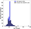 |
Fig. 5. Histogram of the Einstein radii at the source plane for the systems. Blue shows the distribution of all the objects. Grey shows the distribution for the systems with the redshift of the lens known |
In the case of the radius of the accretion disk (RS), it is known that the size obtained by S&S is not in agreement with observational estimates (obtained from reverberation mapping and/or microlensing) and usually underestimates the size of the accretion disk (Morgan et al. 2010; Jiménez-Vicente et al. 2012; Fausnaugh et al. 2018; Jha et al. 2022). To account for this discrepancy, we first calculated the median and standard deviation of the microlensing-based values obtained by Cornachione & Morgan (2020) and Jiménez-Vicente et al. (2012). Then we rescaled all the values to a rest frame of λrest = 2500 Å. Using an MC sampling to estimate the 1σ uncertainties, we obtained a representative experimental median value of RSexp = 1.77 ± 0.41 lt − day. Then we used the ratio between this quantity and the median of our theoretical estimates of RS, based on Eq. (8), RStheor = 0.23 ± 0.003 lt − day, to obtain microlensing corrected RS. The resulting RS values are shown in Fig. 6, with a median of 2.23 ± 0.06 lt−day at 2500 Å after rescaling.
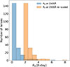 |
Fig. 6. Histogram of the S&S based sizes of the source, RS, before and after applying a microlensing size correction (204 systems). |
The last ingredient to calculate the timescales is the effective velocity of the source (see Sect. 3.2); we present our results in Fig. 7. The median value of the histogram is 807 ± 17 km/s for the systems with known redshifts and 778 ± 10 km/s for the whole sample.
Finally, to make a comparison with M&K results, we first need to rescale our median-corrected source sizes to the wavelength 8140 Å/(1+zS), which is the original wavelength that M&K use to present their results. Our values are given in Fig. 8. From these histograms, we can derive, with 1σ uncertainties, that the mean Einstein ring-crossing time is 11.29 ± 0.05 years for the entire sample and 10.82 ± 0.20 years for the systems with known lens redshifts; whereas M&K obtained a value of 20.6 years. The difference between the two estimates is mainly related to using the updated value for the peculiar velocity at zero redshift by Heß & Kitaura (2016). We notice that Mediavilla et al. (2024), who used a similar approach to estimate the peculiar velocities, obtained an average Einstein radius of 9.4 years, in good agreement with our mean value. On the other hand, for the source crossing timescale, tS, we obtained a mean value of 2.59 ± 0.07 and 2.59 ± 0.09 years for known redshift lens systems and all the sample, respectively. This stands in contrast to the 0.61 years calculated by M&K and this discrepancy arises from both the rescaling of the theoretical sizes and the updated effective velocity.
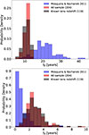 |
Fig. 8. Top: Distribution of Einstein timescales. Bottom: Distribution of source timescales. |
4.3. Microlensing magnification statistics
To explore the possible impact of the source size, rs (rs = 2.07RS), and of the fraction of mass in microlenses, α, on the microlensing magnification statistics, we calculated (for each image of the systems in the sample) magnification maps for two different values of the fraction of mass in microlenses (see Sect. 3.3). These maps were convolved with Gaussian sources of three different sizes, obtaining 2 × 3 different magnification map models (α, rs) and their corresponding magnification histograms. Then, for each of the six individual PDFs obtained for each image, we calculated the mean of the unsigned microlensing magnification values8. In Fig. 9, we present the histograms of these means (520 maps each (α, rs) pair), giving the probability of obtaining an (unsigned) value of microlensing magnification if we were to randomly select one image from the sample. The mean values of these histograms are listed in Table 1. As it can be inferred from Fig. 9, an important difference between the six histograms is the significance of the tail, which is basically ruled by the size of the source (the smaller the size the heavier the tail). This difference may be relevant because there is no evidence of a fat tail in the histograms of observed microlensing magnification (see histogram MED09 in Fig. 1 of Mediavilla et al. 2024). To explore this question in detail, we plot the six histograms in Fig. 10 with a bin size matching that of Mediavilla et al. (2024). This is done for all the images in our sets, for each (α,rs) pair. According to this figure, larger values of the fraction of mass in microlenses and small sizes tend to predict larger magnifications, which were not observed in the MED09 sample. In contrast, small fractions of mass in microlenses and large sizes tend to overpredict low magnifications.
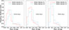 |
Fig. 9. Probability distribution of unsigned microlensing magnification for three different scaling factor values for 0.3 × {rs}, 1.0 × {rs}, and 2.0 × {rs}, with two different stellar densities (α). |
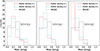 |
Fig. 10. Histogram of unsigned microlensing magnification for three different scaling factors values for rs, with two different stellar densities (α), comparing the results from Mediavilla et al. (2024) and this work, with all histograms normalized to the same total count. |
Mean microlensing statistics for different stellar mass fractions and source-size scaling factors.
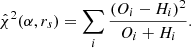
To quantitatively compare the different histograms with MED09, we used the  statistics that takes into account the contribution to the sample variance of both, the modeled and the observed histograms,
 (15)
(15)
Here, Oi and Hi correspond to each bin from the observed histogram, and the modeled one, respectively, from Mediavilla et al. (2024)
The  values obtained are listed in Table 1 and the relative likelihoods of the models, calculated from
  , are represented in Fig. 11. There is a clear minimum in
  , with the maximum probability given in Fig. 11. This corresponds to the model α = 0.2 and set of sizes 1 × {rs}. In Fig. 11 we also plot the contour enclosing a 68% of the probability, which leaves outside the models corresponding to sizes 2 × {rs}. We notice that there is a slight covariance between size and fraction of mass in microlenses in the sense that large sizes can be compensated by high mass fractions and vice versa. Marginalizing on the mass fraction, α, we can obtain an estimate of the expected values for the size, (1.0 ± 0.5)×{rs}, which, taking into account our median value Rs = 2.23 light-days, results in rs = 2.07RS = 4.6 ± 2.3 light-days and in an half-light radius of R1/2 = 2.44RS = 5.4 ± 2.7 light-days. Marginalizing on size, we can infer a lower limit for the fraction of mass in microlenses of α ≥ 0.15 (0.12) in the 68% (90%) confidence interval.
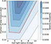 |
Fig. 11. Relative probability distribution (∝e−χ2/2) in the (half light radius [light days], fraction of total mass in stars) parameter space. The red contour marks the 68% confidence region, enclosing the highest-probability values. |
To go further with the statistical analysis of the histograms, we can focus on high magnifications, which are associated to interesting events such as caustic crossings. In Fig. 12 we show the cumulative distribution functions (CDFs) separating the magnifications (Δm < 0) and demagnifications (Δm > 0). The most distinctive feature of these cumulative distributions is the size dependence of the probability of high magnifications. The integrated probability of events with Δm < −0.40 for sizes 0.3 × {rs} is a non-negligible 20% (10%) for α = 0.2 (0.1) while these high magnifications are very unlikely for larger sizes.
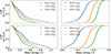 |
Fig. 12. Cumulative distribution functions of magnitude changes during microlensing events. Left column: Probability of observing a demagnification event with Δmag > 0. Right column: Magnification event with Δmag < 0. Top row: Stellar fraction of α = 0.1. Bottom row: α = 0.2. |
To estimate the probability of an HME, in Fig. 13 we plot the probability of having a magnification9Δm ≤ −0.32 and a demagnification Δm ≥ 0.32, respectively. As can be seen in this figure, the probabilities for magnification are dependent on the source size and the fraction of mass in microlenses. On the contrary, there is no significant dependence in the case of demagnification. The mean probabilities for the case (α = 0.2, 1 × {rs}) are 9% (Δm ≤ −0.32) and 26% (Δm ≥ 0.32). When microlensing is detected from a flux ratio, it is not possible, a priori, to separate magnification from demagnification. Consequently, the probability of observing microlensing magnification of an amplitude, |Δm|≥0.32, can be significantly larger (even 35%); however, in at most one-third of the cases, the large degree of magnification might ultimately be shown to be related to a singular magnification event such as a caustic crossing.
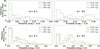 |
Fig. 13. Top: Histogram of the probabilities of obtaining a magnification measurement of less than Δmag = −0.32 for different stellar densities and values of rs. Bottom: Density histogram of the probabilities of obtaining a demagnification greater than Δmag = 0.32 for different stellar densities and values of rs. |
5. Discussion
5.1. Average size of the quasar source and properties of the microlenses population
We found a good matching between the experimental microlensing data from MED09 and the histogram of microlensing magnifications corresponding to the case α = 0.2 and average half-light radius R1/2 = 5.4 light-days modeled by us for the available sample of lenses. These values are in good agreement with previous results from microlensing and reverberation mapping studies. Specifically, from the comparison between histograms, we obtained an estimate of the source size, R1/2 = 5.4 ± 2.7 light-days, which is only slightly affected by the degeneracy with the fraction of mass in microlenses that has been pointed out in other studies. This value for the size is in good agreement with the average size estimate related to reverberation mapping observations (see the discussion in Mediavilla et al. 2017). This result is quite robust, as a significant reduction in size would result in a fat tail of the histogram above Δm ≥ −0.5 not observed in single epoch microlensing measurements (MED09) or in other observations based on light curves (see the histogram PEAKS in Mediavilla et al. 2024). With respect to the mass fraction in microlenses, we estimated a lower limit, α ≥ 0.15, also in good agreement with previous studies (see, e.g., Esteban-Gutiérrez et al. 2022, 2023). To establish more stringent limits, larger values for α should be considered, which implies a computational challenge. We defer this study for future work, although values of α above 0.3 are unexpected.
Regarding the possible existence of a population of intermediate mass black holes (IMBHs) contributing to micro- or millilensing, we note that by virtue of the mass-length degeneracy (see Sect. 1), for relatively high microlensing masses (≳10 M⊙) the quasars will behave as point sources (see, e.g., Esteban-Gutiérrez et al. 2023; Heydenreich et al. 2024). Consequently, a fat tail of high magnifications should be present in the histogram of observations. The absence of this tail excludes the existence of a significant population of BHs above this mass.
Finally, the good matching found between the histogram of magnifications modeled from the full sample of lens systems available and the histogram of observed microlensing magnifications (inferred from just a subset of systems) suggests two key points: (1) the histogram MED09 is statistically representative of microlensing magnification properties of lensed quasar systems and (2) the procedure we followed to infer the magnification statistics (i.e., the lens modeling used to obtain κ and γ for each lensed image) is reliable.
A caveat can be made regarding the comparison with MED09. These data correspond to differential microlensing between pairs of images, which may introduce some broadening of the histogram relative to single-image microlensing. However, the good agreement between MED09 and the distribution of microlensing peaks from light curves (based on single images; see Mediavilla et al. 2024) indicates that this broadening is small compared to other factors, such as intrinsic variability or observational uncertainties.
5.2. Magnification statistics and flux-ratio anomalies
A crucial step in many studies related to multiple imaged quasars is the modeling of the lens. This procedure needs to be very precise, particularly with respect to the prediction of gravitational time delays between the images, which may be used to solve the current tension in the determination of the Hubble constant. However, calculated models very often present strong differences between their predicted flux ratios and the observed ones. These anomalies are often attributed to microlensing. However, the reported model anomalies (see Fig. 1 in Mediavilla et al. 2024) are very high with mean values above 0.5 magnitudes and fat tails reaching even 2.5 magnitudes. According to our statistical study (see Fig. 9), such high levels of magnification have not been predicted even for unexpectedly small source sizes. Thus, we confirm for the present sample the results of previous simulations (Esteban-Gutiérrez et al. 2022; Awad et al. 2023). We provide microlensing magnification histograms for each individual image, which can be used to estimate the potential impact of microlensing on flux ratio anomalies as a criterion for rejecting or accepting a lens model.
5.3. Microlensing timescales and frequency of HME
One main motivation of the statistical study of lens systems is to know the probability of one lens system undergoing high microlensing magnification. In M&K, the answer to this question was based on the comparison between the Einstein and source crossing times. These authors concluded that half of the lensed images will be active with the source lying in the caustic ridges.
Using our microlensing magnification statistics, we can now quantitatively set both the threshold to define an HME and the probability of exceeding it. In Fig. 13, we show the probabilities histogram of having microlensing magnification larger than -0.32, which is the threshold to be within the Einstein ring in the case of an isolated microlens. As shown in Fig. 13, the average probability is around 9% (the average probability of demagnification, Δm ≳ 0.32, associated with smooth variability, is about 26%). We can compare our high magnification probability with the work of Neira et al. (2025), where they estimated the number of HME events with magnification larger than 0.3 Δmag by year for simulated light curves, obtaining ∼60 for 1250 lens quasar images, which is 4.9% per yr, this difference can be associated to the differences in sample and methodology.
It is also interesting to explore the possible correlation between the HME probability and the macro magnification of the image. With this aim, in Fig. 16 we plot the HME probability (i.e., the probability that Δmag < −0.32) versus κ and γ for each image in the sample. From this figure, we can observe (for the smallest size, ×rs = 0.3, considered in the calculations) a clear correlation of the HME probability with the high magnification region defined by the 1 − κ − γ = 0 curve. This correlation disappears for larger values of the source size. The explanation of the correlation observed for ×rs = 0.3 is that a large macro-magnification of the image induce more structure in the microlensing magnification map, increasing the contrast between high magnification ridges and demagnified valleys (see, e.g., Weisenbach et al. 2021, 2024; Neira et al. 2025) and, hence, the probability of HMEs. However, this structure is washed out when convolved with a source of a relatively large size.
On the other hand the origin of the discrepancy with the ∼50% obtained by M&K when comparing tE and tS is that for optical depth close to 1, the real magnification map cannot be understood in terms of a single microdeflector. This is because cooperative effects among microlenses give rise to the highly magnified caustic networks at expenses of other regions, which become demagnified; namely, the scale of regions in the magnification map fulfilling Δm = −0.32 is smaller than one Einstein radius (see Sect. 1).
In Fig. 14, we show a magnification map where the low magnification pixels with Δm > −0.32 have been masked. We notice that the remaining regions appear to be the caustics and inner to caustic regions, and that they occupy just a fraction of the whole map. As discussed above, the apparent "caustics on top of caustics" pattern reflects the densification and overlap of microcaustics for high-macro-magnified images (see Fig. 16), where the caustic network becomes connected and corrugated (see, e.g., Weisenbach et al. 2021, 2024; Neira et al. 2025). We confirmed these results by inspecting magnification maps of 10 images uniformly selected according to the distribution of lensed images in Fig. 15 (top).
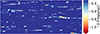 |
Fig. 14. Same convolved microlensing magnification map as in Fig. 2 (right), With a zoom-in between pixel 0 and 400 in the Y axis and full length (1200) in the X axis. Here, the magnification map is masked for values over −0.32, highlighting the regions of strongest magnification within the caustic network. |
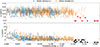 |
Fig. 15. Top: Probability of Δmag ≤ −0.32 versus Einstein radius crossing time (tE [years]), with blue (orange) representing values obtained for a stellar density of 0.1 (0.2) and a 1.0 × {rs}, the red stars represent the object that shows the smaller Einstein radius crossing time and high magnification probability that correspond to DESJ2038-4008 and Q2237+030. Bottom: Probability or Δmag ≤ −0.32 versus source crossing time (tS [years]), with blue (orange) representing values obtained for a stellar density of 0.1 (0.2) and a RS× 1, in black stars the objects that show the smallest source crossing time and hight probability that are CY2201-3201, WG2100-4452, SDSSJ1138+0314, SDSSJ0821+4542, J0343-2828, WG0214-2105, and Q2237+030. |
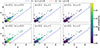 |
Fig. 16. Correlation between the values of κ and γ in our sample, with the color bar representing the HME probability. The panels are separated by α and by multiples of rs. |
In Fig. 15 we show, for each one of the images of lens systems in our sample, the probability of microlensing magnification above –0.32 mag vs. crossing times. If we are interested in caustic scanning of the accretion disk or the innermost region of the BLR (Fian et al. 2024), we can select the objects with the highest probability and smaller source crossing time as candidates; for instance, CY2201-3201, WG2100-4452, SDSSJ1138+0314, SDSSJ0821+4542, J0343-2828, WG0214-2105, and Q2237+030. If we are interested in estimating any pseudo-periodical property of microlensing (e.g., the caustic crossing frequency related to the peculiar velocity of the lens galaxy, see Mediavilla et al. 2016), we should instead select systems with smaller Einstein radius crossing times; for instance: DESJ2038-4008 and Q2237+030.
6. Conclusions
With the aim of conducting a statistical study of some relevant properties of quasar microlensing, we collected data from all known lensed quasar systems and performed a comprehensive and homogeneous modeling of gravitational lensing systems to estimate key parameters. In particular, we used the Einstein radius of the lensed systems, along with the convergence (κ) and shear (γ) of the lensed quasar images. From κ and γ, we obtained microlensing magnification maps for all the images using two values for stellar density (0.1 and 0.2). We combined the available data and calculations to estimate the microlensing magnification probabilities and crossing times. Our main results are as follows.
1. Our lens fitting procedure displayed a high level of agreement with previous studies. In particular, when compared with the sample of lensed quasars compiled by Amante et al. (2020), we found that 88% of the systems are consistent within our estimated uncertainties. Further comparisons with automatic modeling studies, such as those performed by Schmidt et al. (2023), who used LENSTRONOMY on 30 quadruply lensed quasars, showed a good concordance for 21 out of 29 common systems. Similarly, when compared with models from GLEE, our results were in agreement to within 2 σ for seven out of eight systems, reinforcing the reliability of our modeling approach.
2. We compared the observed microlensing magnification histogram with the magnification histogram of our sample of 204 lensed quasar systems modeled for different values of the fraction of mass in microlenses, α, and the size of the quasar source. We obtained a Bayesian estimate of the average half-light radius of R1/2 = 5.4 ± 2.7 light days and a lower limit of α ≥ 0.15, in excellent agreement with previous studies based on microlensing and reverberation mapping.
3. According to the histogram of mean magnifications, it is unlikely that microlensing would lead to overall flux-ratio anomalies above ∼0.3 mag. Thus, lens modeling leading to larger flux-ratio anomalies should be regarded with caution; particularly in the context of Hubble constant estimate from lensed quasar monitoring. The individual microlensing magnification PDFs we provide here are available upon request for each image. These data can be used to cross-check lens models by comparing the resulting flux-ratio anomalies with the predicted microlensing.
4. We found a median timescale of tE = 11.29 ± 0.05 years for the Einstein radius crossing time and tS = 2.59 ± 0.07 years for the source size crossing time after accounting for uncertainties through MC simulations. These values differ from those reported by M&K, who found median values of 20 years and 0.61 years, respectively. The discrepancies can be mainly attributed to differences in the methodologies for calculating effective velocities and to our rescaling of the theoretical accretion disk sizes to account for recent measurements based on reverberation mapping and microlensing.
5. Beyond the single particle-based analysis of the Einstein radius crossing time, the study of microlensing magnification maps and histograms enables us to obtain more detailed and quantitative information about the probability of observing some interesting phenomenology related to microlensing, such as caustic crossing. Specifically, due to the formation of caustics networks, the size of the regions with magnification Δm ≤ −0.32 (corresponding to the region inner to the Einstein radius of one isolated particle) is significantly smaller than the Einstein radius. We find that these regions correspond to the caustic and (partly) to the inner to caustic locations. We also find that these regions occupy, on average, 9% of the magnification maps (i.e., if you randomly pick an image from our sample, this is the rough probability of this image being engaged in a past or future caustic crossing event). In agreement with previous studies (see, e.g., Weisenbach et al. 2021, 2024; Neira et al. 2025), we find a correlation between the macro-magnification of the image and the probability of HMEs for sources of relatively small sizes.
6. Combining the crossing times with the probabilities of a high magnification event, we were able to determine the best candidates for dissecting the structure of accretion disks through caustic scanning and studying the statistics of pseudo-periodical magnification events (e.g., caustic or zero crossings). This work provides a homogeneous statistical framework for linking lens-model parameters with microlensing observables in the current population of known lensed quasars. The resulting magnification maps, probability distributions, and timescales provide a reference for interpreting flux-ratio anomalies and for selecting the most promising systems for future microlensing monitoring. This approach will be particularly valuable in the context of the larger lensed quasar samples expected from ongoing and upcoming wide-field surveys.
Data availability
In the body of the paper, we presented figures and results for the scales, effective velocity, source sizes, and magnification map statistics. We provide an online appendix at https://github.com/felavila/microlensing-Maps-Post-Analysis-results.
Acknowledgments
We thank Jorge Jiménez Vicente (†) for his valuable help and insightful comments. FAV thanks the Doctorate Fellowship program FIB-UV of the Universidad de Valparaíso for funding, ESO Early-Career Visitor Programme and the ESO Science Support Discretionary Fund. This work was supported by ANID FONDECYT Regular grant number 1231418 (VM, FAV) and by the Centro de Astrofísica de Valparaíso (CIDI 21). EM acknowledges support from grants PID2020-118687GB-C31 and PID2020-118687GB-C33, financed by the Spanish Ministerio de Ciencia e Innovación/Agencia Estatal de Investigación MCIN/AEI/10.13039/501100011033.
References
- Abajas, C., Mediavilla, E., Muñoz, J. A., Popović, L. Č., & Oscoz, A. 2002, ApJ, 576, 640 [Google Scholar]
- Agnello, A., Grillo, C., Jones, T., et al. 2018, MNRAS, 474, 3391 [CrossRef] [Google Scholar]
- Amante, M. H., Magaña, J., Motta, V., García-Aspeitia, M. A., & Verdugo, T. 2020, MNRAS, 498, 6013 [Google Scholar]
- Andika, I. T., Schuldt, S., Suyu, S. H., et al. 2025, A&A, 694, A227 [NASA ADS] [CrossRef] [EDP Sciences] [Google Scholar]
- Anguita, T., Schmidt, R. W., Turner, E. L., et al. 2008, A&A, 480, 327 [NASA ADS] [CrossRef] [EDP Sciences] [Google Scholar]
- Avila, F., Bernui, A., Nunes, R. C., de Carvalho, E., & Novaes, C. P. 2022, MNRAS, 509, 2994 [Google Scholar]
- Awad, P., Chan, J. H. H., Millon, M., Courbin, F., & Paic, E. 2023, A&A, 673, A88 [NASA ADS] [CrossRef] [EDP Sciences] [Google Scholar]
- Birrer, S., & Amara, A. 2018, Phys. Dark Univ., 22, 189 [Google Scholar]
- Birrer, S., Amara, A., & Refregier, A. 2015, ApJ, 813, 102 [Google Scholar]
- Blandford, R. D., & Narayan, R. 1992, ARA&A, 30, 311 [NASA ADS] [CrossRef] [Google Scholar]
- Bonaca, A., Conroy, C., Wetzel, A., Hopkins, P. F., & Kereš, D. 2017, ApJ, 845, 101 [NASA ADS] [CrossRef] [Google Scholar]
- Chan, J. H. H., Wong, K. C., Ding, X., et al. 2024, MNRAS, 527, 6253 [Google Scholar]
- Coe, D., & Moustakas, L. A. 2009, ApJ, 706, 45 [Google Scholar]
- Collett, T. E. 2015, ApJ, 811, 20 [NASA ADS] [CrossRef] [Google Scholar]
- Cornachione, M. A., & Morgan, C. W. 2020, ApJ, 895, 93 [Google Scholar]
- Di Valentino, E., Mena, O., Pan, S., et al. 2021, CQG, 38, 153001 [NASA ADS] [CrossRef] [Google Scholar]
- Dux, F., Millon, M., Lemon, C., et al. 2025, A&A, 694, A300 [NASA ADS] [CrossRef] [EDP Sciences] [Google Scholar]
- Erickson, S., Wagner-Carena, S., Marshall, P., et al. 2025, AJ, 170, 44 [Google Scholar]
- Ertl, S., Schuldt, S., Suyu, S. H., et al. 2023, A&A, 672, A2 [NASA ADS] [CrossRef] [EDP Sciences] [Google Scholar]
- Esteban-Gutiérrez, A., Agües-Paszkowsky, N., Mediavilla, E., et al. 2022, ApJ, 929, 123 [CrossRef] [Google Scholar]
- Esteban-Gutiérrez, A., Mediavilla, E., Jiménez-Vicente, J., & Muñoz, J. A. 2023, ApJ, 954, 172 [CrossRef] [Google Scholar]
- Fagin, J., Park, J. W., Best, H., et al. 2024, ApJ, 965, 104 [Google Scholar]
- Fausnaugh, M. M., Starkey, D. A., Horne, K., et al. 2018, ApJ, 854, 107 [NASA ADS] [CrossRef] [Google Scholar]
- Fian, C., Guerras, E., Mediavilla, E., et al. 2018, ApJ, 859, 50 [Google Scholar]
- Fian, C., Mediavilla, E., Jiménez-Vicente, J., et al. 2021, A&A, 654, A70 [NASA ADS] [CrossRef] [EDP Sciences] [Google Scholar]
- Fian, C., Muñoz, J. A., Forés-Toribio, R., et al. 2024, A&A, 682, A57 [NASA ADS] [CrossRef] [EDP Sciences] [Google Scholar]
- Gil-Merino, R., & Lewis, G. F. 2005, A&A, 437, L15 [NASA ADS] [CrossRef] [EDP Sciences] [Google Scholar]
- Grillo, C., Lombardi, M., & Bertin, G. 2008, A&A, 477, 397 [NASA ADS] [CrossRef] [EDP Sciences] [Google Scholar]
- Hagen, H. J., & Reimers, D. 2000, A&A, 357, L29 [Google Scholar]
- Heß, S., & Kitaura, F.-S. 2016, MNRAS, 456, 4247 [Google Scholar]
- Heydenreich, S., Mediavilla, E., Jiménez-Vicente, J., Vives-Arias, H., & Muñoz, J. A. 2024, A&A, 690, A307 [NASA ADS] [CrossRef] [EDP Sciences] [Google Scholar]
- Holtzman, J. A., Watson, A. M., Baum, W. A., et al. 1998, AJ, 115, 1946 [Google Scholar]
- Hutsemékers, D., Sluse, D., & Savić, {D}. 2024, A&A, 691, A292 [NASA ADS] [CrossRef] [EDP Sciences] [Google Scholar]
- Ivezić, Ž., Kahn, S. M., Tyson, J. A., et al. 2019, ApJ, 873, 111 [Google Scholar]
- Jha, V. K., Joshi, R., Chand, H., et al. 2022, MNRAS, 511, 3005 [NASA ADS] [CrossRef] [Google Scholar]
- Jiménez-Vicente, J., & Mediavilla, E. 2019, ApJ, 885, 75 [Google Scholar]
- Jiménez-Vicente, J., & Mediavilla, E. 2022, ApJ, 941, 80 [CrossRef] [Google Scholar]
- Jiménez-Vicente, J., & Mediavilla, E. 2025, MNRAS, 541, 1264 [Google Scholar]
- Jiménez-Vicente, J., Mediavilla, E., Muñoz, J. A., & Kochanek, C. S. 2012, ApJ, 751, 106 [Google Scholar]
- Jiménez-Vicente, J., Mediavilla, E., Kochanek, C. S., et al. 2014, ApJ, 783, 47 [Google Scholar]
- Jiménez-Vicente, J., Mediavilla, E., Kochanek, C. S., & Muñoz, J. A. 2015, ApJ, 799, 149 [Google Scholar]
- Kayser, R., Refsdal, S., & Stabell, R. 1986, A&A, 166, 36 [NASA ADS] [Google Scholar]
- Keeton, C. R. 2001a, ArXiv e-prints [arXiv:astro-ph/0102341] [Google Scholar]
- Keeton, C. R. 2001b, ArXiv e-prints [arXiv:astro-ph/0102340] [Google Scholar]
- Keeton, C. R. 2011, Astrophysics Source Code Library [record ascl:1102.003] [Google Scholar]
- Knabel, S., Mozumdar, P., Shajib, A. J., et al. 2025, ApJ, 703, A117 [Google Scholar]
- Kochanek, C. S. 2004, ApJ, 605, 58 [Google Scholar]
- Kormann, R., Schneider, P., & Bartelmann, M. 1994, A&A, 284, 285 [NASA ADS] [Google Scholar]
- Krone-Martins, A., Delchambre, L., Wertz, O., et al. 2018, A&A, 616, L11 [NASA ADS] [CrossRef] [EDP Sciences] [Google Scholar]
- Lefor, A. T., Futamase, T., & Akhlaghi, M. 2013, New Astron. Rev., 57, 1 [CrossRef] [Google Scholar]
- Leier, D., Ferreras, I., Saha, P., & Falco, E. E. 2011, ApJ, 740, 97 [NASA ADS] [CrossRef] [Google Scholar]
- Lemon, C. A., Auger, M. W., McMahon, R. G., & Koposov, S. E. 2017, MNRAS, 472, 5023 [NASA ADS] [CrossRef] [Google Scholar]
- Lemon, C. A., Auger, M. W., McMahon, R. G., & Ostrovski, F. 2018, MNRAS, 479, 5060 [Google Scholar]
- Lemon, C., Anguita, T., Auger-Williams, M. W., et al. 2023, MNRAS, 520, 3305 [NASA ADS] [CrossRef] [Google Scholar]
- Lucey, J. R., Schechter, P. L., Smith, R. J., & Anguita, T. 2018, MNRAS, 476, 927 [NASA ADS] [CrossRef] [Google Scholar]
- Mao, S. 2012, Res. Astron. Astrophys., 12, 947 [Google Scholar]
- Mediavilla, E., Muñoz, J. A., Lopez, P., et al. 2006, ApJ, 653, 942 [NASA ADS] [CrossRef] [Google Scholar]
- Mediavilla, E., Muñoz, J. A., Falco, E., et al. 2009, ApJ, 706, 1451 [NASA ADS] [CrossRef] [Google Scholar]
- Mediavilla, E., Mediavilla, T., Muñoz, J. A., et al. 2011, ApJ, 741, 42 [NASA ADS] [CrossRef] [Google Scholar]
- Mediavilla, E., Jiménez-vicente, J., Muñoz, J. A., & Mediavilla, T. 2015, ApJ, 814, L26 [NASA ADS] [CrossRef] [Google Scholar]
- Mediavilla, E., Jiménez-Vicente, J., Muñoz, J. A., & Battaner, E. 2016, ApJ, 832, 46 [CrossRef] [Google Scholar]
- Mediavilla, E., Jiménez-Vicente, J., Muñoz, J. A., Vives-Arias, H., & Calderón-Infante, J. 2017, ApJ, 836, L18 [NASA ADS] [CrossRef] [Google Scholar]
- Mediavilla, E., Jiménez-Vicente, J., & Motta, V. 2024, AJ, 167, 171 [NASA ADS] [CrossRef] [Google Scholar]
- Morgan, C. W., Kochanek, C. S., Morgan, N. D., & Falco, E. E. 2010, ApJ, 712, 1129 [Google Scholar]
- Morgan, C. W., Hyer, G. E., Bonvin, V., et al. 2018, ApJ, 869, 106 [Google Scholar]
- Mortonson, M. J., Schechter, P. L., & Wambsganss, J. 2005, ApJ, 628, 594 [NASA ADS] [CrossRef] [Google Scholar]
- Mosquera, A. M., & Kochanek, C. S. 2011, ApJ, 738, 96 [Google Scholar]
- Muñoz, J. A., Falco, E. E., Kochanek, C. S., et al. 1998, Ap&SS, 263, 51 [Google Scholar]
- Neira, F., Anguita, T., & Vernardos, G. 2020, MNRAS, 495, 544 [NASA ADS] [CrossRef] [Google Scholar]
- Neira, F., Anguita, T., & Vernardos, G. 2025, A&A, 701, A35 [NASA ADS] [CrossRef] [EDP Sciences] [Google Scholar]
- Nightingale, J., Hayes, R., Kelly, A., et al. 2021, J. Open Source Software, 6, 2825 [NASA ADS] [CrossRef] [Google Scholar]
- Oguri, M., & Marshall, P. J. 2010, MNRAS, 405, 2579 [NASA ADS] [Google Scholar]
- Paczynski, B. 1986, ApJ, 304, 1 [NASA ADS] [CrossRef] [Google Scholar]
- Paic, E., Vernardos, G., Sluse, D., et al. 2022, A&A, 659, A21 [NASA ADS] [CrossRef] [EDP Sciences] [Google Scholar]
- Pindor, B., Eisenstein, D. J., Inada, N., et al. 2004, AJ, 127, 1318 [NASA ADS] [CrossRef] [Google Scholar]
- Planck Collaboration I. 2020, A&A, 641, A1 [NASA ADS] [CrossRef] [EDP Sciences] [Google Scholar]
- Poindexter, S., & Kochanek, C. S. 2010, ApJ, 712, 658 [NASA ADS] [CrossRef] [Google Scholar]
- Redlich, M., Bartelmann, M., Waizmann, J. C., & Fedeli, C. 2012, A&A, 547, A66 [NASA ADS] [CrossRef] [EDP Sciences] [Google Scholar]
- Refsdal, S., & Stabell, R. 1997, A&A, 325, 877 [NASA ADS] [Google Scholar]
- Robertson, A., Smith, G. P., Massey, R., et al. 2020, MNRAS, 495, 3727 [NASA ADS] [CrossRef] [Google Scholar]
- Rodrigo, C., & Solano, E. 2020, in XIV.0 Scientific Meeting (virtual) of the Spanish Astronomical Society, 182 [Google Scholar]
- Rojas, K., Motta, V., Mediavilla, E., et al. 2014, ApJ, 797, 61 [Google Scholar]
- Schmidt, T., Treu, T., Birrer, S., et al. 2023, MNRAS, 518, 1260 [Google Scholar]
- Schneider, P., Ehlers, J., & Falco, E. E. 1992, Gravitational Lenses, 560, 112 [Google Scholar]
- Shajib, A. J., Wong, K. C., Birrer, S., et al. 2022, A&A, 667, A123 [NASA ADS] [CrossRef] [EDP Sciences] [Google Scholar]
- Shajib, A. J., Vernardos, G., Collett, T. E., et al. 2024, Space Sci. Rev., 220, 87 [CrossRef] [Google Scholar]
- Shakura, N. I., & Sunyaev, R. A. 1973, A&A, 24, 337 [NASA ADS] [Google Scholar]
- Sluse, D., Kishimoto, M., Anguita, T., Wucknitz, O., & Wambsganss, J. 2013, A&A, 553, A53 [NASA ADS] [CrossRef] [EDP Sciences] [Google Scholar]
- Smith, M. C., Evans, N. W., Belokurov, V., et al. 2009, MNRAS, 399, 1223 [Google Scholar]
- Suyu, S. H., Marshall, P. J., Auger, M. W., et al. 2010, ApJ, 711, 201 [Google Scholar]
- Treu, T. 2010, ARA&A, 48, 87 [NASA ADS] [CrossRef] [Google Scholar]
- The Dark Energy Survey Collaboration 2005, ArXiv e-prints [arXiv:astro-ph/0510346] [Google Scholar]
- Treu, T., Gavazzi, R., Gorecki, A., et al. 2009, ApJ, 690, 670 [NASA ADS] [CrossRef] [Google Scholar]
- Treu, T., Agnello, A., Baumer, M. A., et al. 2018, MNRAS, 481, 1041 [NASA ADS] [CrossRef] [Google Scholar]
- Tully, R. B. 2023, ArXiv e-prints [arXiv:2305.11950] [Google Scholar]
- Verde, L., Schöneberg, N., & Gil-Marín, H. 2024, ARA&A, 62, 287 [Google Scholar]
- Vernardos, G., & Fluke, C. J. 2013, MNRAS, 434, 832 [Google Scholar]
- Vernardos, G., Fluke, C. J., Bate, N. F., & Croton, D. 2014, ApJS, 211, 16 [NASA ADS] [CrossRef] [Google Scholar]
- Vernardos, G., Fluke, C. J., Bate, N. F., Croton, D., & Vohl, D. 2015, ApJS, 217, 23 [CrossRef] [Google Scholar]
- Vernardos, G., Sluse, D., Pooley, D., et al. 2024, Space Sci. Rev., 220, 14 [NASA ADS] [CrossRef] [Google Scholar]
- Vives-Arias, H., Muñoz, J. A., Kochanek, C. S., Mediavilla, E., & Jiménez-Vicente, J. 2016, ApJ, 831, 43 [NASA ADS] [CrossRef] [Google Scholar]
- Walsh, D., Carswell, R. F., & Weymann, R. J. 1979, Nature, 279, 381 [Google Scholar]
- Wambsganss, J. 2006, ArXiv e-prints [arXiv:astro-ph/0604278] [Google Scholar]
- Weisenbach, L. 2025, MNRAS, 541, 281 [Google Scholar]
- Weisenbach, L., Schechter, P. L., & Pontula, S. 2021, ApJ, 922, 70 [NASA ADS] [CrossRef] [Google Scholar]
- Weisenbach, L., Anguita, T., Miralda-Escudé, J., et al. 2024, Space Sci. Rev., 220, 57 [Google Scholar]
- Wildy, C., & Czerny, B. 2017, Front. Astron. Space. Sciences, 4, 43 [Google Scholar]
- Wyithe, J. S. B., & Turner, E. L. 2001, MNRAS, 320, 21 [Google Scholar]
- Wyithe, J. S. B., & Turner, E. L. 2002, ApJ, 575, 650 [Google Scholar]
As discussed in Sect. 2, the empirical histogram of microlensing magnifications from Mediavilla et al. (2009, 2024), which we use to compare predictions with observations, is based on single-epoch measurements that do not determine the sign and are derived from image pairs, whereas our values are derived from individual quasar images.
We select the umbral magnification Δm = −0.32, as it is the value at the Einstein ring of an isolated particle.
All Tables
Mean microlensing statistics for different stellar mass fractions and source-size scaling factors.
All Figures
|
Fig. 1. Astrometric error distribution for the sample of images modeled. |
| In the text | |
|
Fig. 2. Microlensing magnification patterns produced by stars in the lensing galaxy corresponding to image A of the system DES2158−5812. Left: Original magnification map. The color scale encodes different magnification levels, while the diamond-shaped curves trace the caustics. Right: Same map after convolution with a Gaussian profile with a sigma size of 3.72 [pix], showing the effective magnification pattern. Both panels have a size of 1200 × 1200 pixels with a pixel size of 1.1 [pix/light-days] and 60 RE. The maps were produced using the code developed in Jiménez-Vicente & Mediavilla (2022). |
| In the text | |
|
Fig. 3. Comparison of θE in this work vs. values in the literature for modeled lens quasars. The systems that are clearly far from a 1:1 relation are SDSS 1155+6346 and HS 0818+1227. |
| In the text | |
|
Fig. 4. Values of κ and γ for our sample (red filled diamonds), compared with literature samples: unfilled black diamonds Neira et al. (2025), unfilled circles Ertl et al. (2023), and unfilled black squares Schmidt et al. (2023). |
| In the text | |
|
Fig. 5. Histogram of the Einstein radii at the source plane for the systems. Blue shows the distribution of all the objects. Grey shows the distribution for the systems with the redshift of the lens known |
| In the text | |
|
Fig. 6. Histogram of the S&S based sizes of the source, RS, before and after applying a microlensing size correction (204 systems). |
| In the text | |
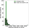 |
Fig. 7. Histogram of the distribution of the effective velocities (Eq. (10)). |
| In the text | |
|
Fig. 8. Top: Distribution of Einstein timescales. Bottom: Distribution of source timescales. |
| In the text | |
|
Fig. 9. Probability distribution of unsigned microlensing magnification for three different scaling factor values for 0.3 × {rs}, 1.0 × {rs}, and 2.0 × {rs}, with two different stellar densities (α). |
| In the text | |
|
Fig. 10. Histogram of unsigned microlensing magnification for three different scaling factors values for rs, with two different stellar densities (α), comparing the results from Mediavilla et al. (2024) and this work, with all histograms normalized to the same total count. |
| In the text | |
|
Fig. 11. Relative probability distribution (∝e−χ2/2) in the (half light radius [light days], fraction of total mass in stars) parameter space. The red contour marks the 68% confidence region, enclosing the highest-probability values. |
| In the text | |
|
Fig. 12. Cumulative distribution functions of magnitude changes during microlensing events. Left column: Probability of observing a demagnification event with Δmag > 0. Right column: Magnification event with Δmag < 0. Top row: Stellar fraction of α = 0.1. Bottom row: α = 0.2. |
| In the text | |
|
Fig. 13. Top: Histogram of the probabilities of obtaining a magnification measurement of less than Δmag = −0.32 for different stellar densities and values of rs. Bottom: Density histogram of the probabilities of obtaining a demagnification greater than Δmag = 0.32 for different stellar densities and values of rs. |
| In the text | |
|
Fig. 14. Same convolved microlensing magnification map as in Fig. 2 (right), With a zoom-in between pixel 0 and 400 in the Y axis and full length (1200) in the X axis. Here, the magnification map is masked for values over −0.32, highlighting the regions of strongest magnification within the caustic network. |
| In the text | |
|
Fig. 15. Top: Probability of Δmag ≤ −0.32 versus Einstein radius crossing time (tE [years]), with blue (orange) representing values obtained for a stellar density of 0.1 (0.2) and a 1.0 × {rs}, the red stars represent the object that shows the smaller Einstein radius crossing time and high magnification probability that correspond to DESJ2038-4008 and Q2237+030. Bottom: Probability or Δmag ≤ −0.32 versus source crossing time (tS [years]), with blue (orange) representing values obtained for a stellar density of 0.1 (0.2) and a RS× 1, in black stars the objects that show the smallest source crossing time and hight probability that are CY2201-3201, WG2100-4452, SDSSJ1138+0314, SDSSJ0821+4542, J0343-2828, WG0214-2105, and Q2237+030. |
| In the text | |
|
Fig. 16. Correlation between the values of κ and γ in our sample, with the color bar representing the HME probability. The panels are separated by α and by multiples of rs. |
| In the text | |
Current usage metrics show cumulative count of Article Views (full-text article views including HTML views, PDF and ePub downloads, according to the available data) and Abstracts Views on Vision4Press platform.
Data correspond to usage on the plateform after 2015. The current usage metrics is available 48-96 hours after online publication and is updated daily on week days.
Initial download of the metrics may take a while.