Mechanisms for magnetic braking boost and disruption: The role of irradiation-driven winds and the convective turnover time spike in cataclysmic variables

Vladislav Dodon; Xiang-Dong Li; Xiao-jie Xu; Ilkham Galiullin; Askar Sibgatullin

doi:10.1051/0004-6361/202660098

Home

All issues

Volume 710 (June 2026)

A&A, 710 (2026) A317

Full HTML

Open Access

Issue		A&A Volume 710, June 2026


Article Number		A317
Number of page(s)		15
Section		Stellar structure and evolution
DOI		https://doi.org/10.1051/0004-6361/202660098
Published online		24 June 2026

A&A, 710, A317 (2026)

Mechanisms for magnetic braking boost and disruption: The role of irradiation-driven winds and the convective turnover time spike in cataclysmic variables

Vladislav Dodon¹^,2^★, Xiang-Dong Li¹, Xiao-jie Xu¹, Ilkham Galiullin² and Askar Sibgatullin²

¹ School of Astronomy and Space Science, Nanjing University, Nanjing 210023, PR China
² Kazan Federal University, Kremlevskaya Str.18, 420008 Kazan, Russia

^★ Corresponding authors: This email address is being protected from spambots. You need JavaScript enabled to view it.

Received: 27 March 2026
Accepted: 13 May 2026

Abstract

Context. The saturated, boosted, and disrupted (SBD) magnetic braking (MB) model is an empirical prescription that has recently gained support from observations of diverse close binary systems. Different boosting (K) and disruption (η) parameters appear necessary for different systems, but their physical origins remain uncertain.

Aims. We aim to identify the physical mechanisms that boost MB and cause its disruption at the fully convective boundary in cataclysmic variables (CVs).

Methods. We modelled CV evolution using the MESA code and compared the results with observed CV properties. We computed the convective turnover time (τ_c) directly from the donor’s structure rather than adopting empirical relations. We also included irradiation from the accreting white dwarf, which heats the donor’s outer layers and can drive additional winds that enhance MB.

Results. The structure-based τ_c calculation reveals a pronounced spike as the donor approaches full convection, which drives the disruption parameter (η) and initiates the period gap in CVs. The outcome of irradiation is sensitive to the accretion, irradiation, and wind efficiencies, as well as to the base wind mass-loss rate of M-dwarf donors, all of which are poorly constrained from observations. Despite these uncertainties, plausible parameter choices allow irradiation-driven winds to provide the required boost (K) during accreting phases. We refer to the combined prescription as the iτSBD MB model and find that it yields evolutionary tracks broadly consistent with the main CV properties.

Conclusions. Our iτSBD MB framework offers a physically motivated interpretation of the empirical boost and disruption factors in SBD MB for CV evolution. We suggest that the convective turnover time spike at the fully convective boundary may be the universal driver of MB disruption for fast-rotating stars in the saturated regime, while irradiation-driven winds may be the dominant mechanism boosting MB in accreting binaries and other strongly irradiated close systems.

Key words: methods: numerical / binaries: close / stars: evolution / novae / cataclysmic variables / X-rays: binaries

© The Authors 2026

Open Access article, published by EDP Sciences, under the terms of the Creative Commons Attribution License (https://creativecommons.org/licenses/by/4.0), which permits unrestricted use, distribution, and reproduction in any medium, provided the original work is properly cited.

This article is published in open access under the Subscribe to Open model. This email address is being protected from spambots. You need JavaScript enabled to view it. to support open access publication.

1. Introduction

Magnetic braking (MB) is the principal angular momentum loss (AML) mechanism that governs the spin-down of low-mass single stars and the secular evolution of many close binaries (Schatzman 1962; Weber & Davis 1967; Mestel 1968). In essence, the stellar magnetic field forces its outflowing wind to co-rotate out to the Alfvén radius, so the escaping matter removes angular momentum with a much larger lever arm. The predictable spin-down produced by MB forms the basis of gyrochronology, which uses stellar rotation as an age indicator (Skumanich 1972; Barnes 2003, 2007). In tidally locked binary stars, the torque is removed from the orbital angular momentum, causing the binary to shrink. As a result, MB is efficient in bringing detached binaries into contact, thereby giving rise to accretion-powered systems such as low-mass X-ray binaries (LMXBs) and cataclysmic variables (CVs; Verbunt & Zwaan 1981; Rappaport et al. 1983).

Despite its simple physical picture, MB is a complex process as it depends on the wind mass-loss rate, magnetic field strength and topology, and the dynamo’s response to rotation and convection, all of which vary across spectral type and evolutionary state (Matt et al. 2012; Réville et al. 2015; Matt et al. 2015). Historically, different MB prescriptions have been developed for particular stellar regimes or observational constraints (e.g. Verbunt & Zwaan 1981; Kawaler 1988; Andronov et al. 2003; Garraffo et al. 2018; Van & Ivanova 2019). In particular, the prescription of Rappaport et al. (1983, hereafter RVJ) was adopted extensively in binary evolution studies and underpinned many standard evolutionary models of CVs and LMXBs (Tauris & Savonije 1999; Howell et al. 2001; Podsiadlowski et al. 2002). When extrapolated beyond their calibration domain, MB prescriptions often disagree by orders of magnitude (e.g. Knigge et al. 2011; Deng et al. 2021; El-Badry et al. 2022; Gossage et al. 2023; Zhou et al. 2026). This lack of universality poses a major obstacle to evolutionary modelling, because the MB torque cannot be predicted reliably across different physical regimes. Additional complications arise in exotic cases such as strongly magnetic CVs, where MB is significantly reduced because of the coupling of the donor and white dwarf (WD) magnetospheres (Li et al. 1994; Belloni et al. 2020). There is currently no universal MB recipe able to predict the evolution of all systems consistently.

Cataclysmic variables can serve as useful laboratories for testing MB prescriptions. They are compact semi-detached binaries consisting of an accreting WD and a Roche lobe filling companion star (Warner 2003). CVs are also X-ray sources, with typical luminosities spanning L_X ∼ 10²⁹ − 10³² erg s⁻¹ (see e.g. Mukai 2017; Galiullin et al. 2024). The long-term evolution of CVs is governed by AML (Belloni & Schreiber 2023), mainly through MB and gravitational radiation (GR; Paczyński 1967; Patterson 1984). Additional consequential angular momentum loss (CAML) is needed to account for the material leaving the system during nova eruptions (King & Kolb 1995). In the standard evolutionary picture of non-magnetic, hydrogen-rich CVs, MB dominates at longer orbital periods (see e.g. Knigge et al. 2011). At a period of ∼3 h, the donor star becomes fully convective and the MB strength suddenly drops. This abrupt change in AML can initiate a detached phase, leaving the resulting WD+M-dwarf binaries effectively unobservable and giving rise to the so-called period gap (Spruit & Ritter 1983). The remaining GR shrinks the orbit to a period of ∼2 h, at which point the donor fills its Roche lobe again and accretion restarts. At a period of ∼80 min, the donor reaches a mass of ∼0.08 M_⊙ and becomes a degenerate brown dwarf (Kolb & Baraffe 1999). The response of the degenerate donor to mass loss then changes, leading to an increase in the orbital period. The period gap at ∼2 − 3 h and period minimum at ∼80 min are robust features of the CV period distribution and can serve as key diagnostics for testing new stellar physics (Schreiber et al. 2024).

A recent development towards a more unified description of MB is the saturated, boosted, and disrupted (SBD) MB prescription introduced by Belloni et al. (2024). It builds on the notion that MB saturates at shorter rotation periods; studies of different binaries in recent years have provided additional robust evidence of this (El-Badry et al. 2022; Fabry & Prša 2025). Two additional multiplicative factors are introduced: one that boosts the braking strength above the fully convective boundary (K) and one that disrupts it once the donor becomes fully convective (η). While Belloni et al. (2024) originally studied detached post-common-envelope WD+M-dwarf binaries, the SBD MB prescription has recently gained further support from studies of hot subdwarf B (sdB) plus main-sequence (MS) binaries (Blomberg et al. 2024) and CVs (Barraza-Jorquera et al. 2025). Its apparent success across diverse binaries suggests that SBD MB may provide the basis for a more unified description of MB. However, the model remains essentially empirical, and the physical origin of the boost and disruption terms is still unclear. Previous SBD MB studies assumed constant values with K ≃ η along the binary evolution, but the two factors likely reflect different underlying mechanisms.

Two possibilities appear particularly worth exploring. Blomberg et al. (2024) propose that the boost arises from irradiation-enhanced winds of the MS star, and Barraza-Jorquera et al. (2025) suggest that the empirical treatment of the convective turnover time (τ_c) is a weak point of the model. On the one hand, the disrupted MB term η should be connected to structural changes in the donor as it approaches the fully convective boundary, where τ_c is also expected to change abruptly (Gossage et al. 2025). On the other hand, it is known that in close accreting binaries, accretion onto the compact object produces strong X-ray emission that can significantly heat the donor-facing side and induce a considerable stellar wind (Basko & Sunyaev 1973; Basko et al. 1974; Iben et al. 1997). Such an irradiation-driven outflow may add significantly to the donor’s intrinsic wind, thereby enhancing the mass loss that powers ordinary MB. In this study, we investigated whether these two mechanisms can account for the boost and disruption of MB in CVs by developing a physically motivated model and testing it with binary evolution calculations.

During the final stage of preparing this manuscript, Barraza-Jorquera et al. (2026) revised the SBD MB model for CVs using the saturated prescription of Matt et al. (2015). They recalculated the global convective turnover time directly from the stellar structure, revised the saturation threshold, and found that, in this formulation, smaller empirical boost and disruption factors are sufficient to reproduce the main CV properties. Our results support the idea that the treatment of τ_c is crucial and do not contradict the conclusions of Barraza-Jorquera et al. (2026). At the same time, using the original SBD MB formulation, we show that donor-structure effects in τ_c can directly drive MB disruption in saturated prescriptions that retain an explicit τ_c dependence, while irradiation-driven winds provide a plausible source of the remaining boost.

This paper is organised as follows. Section 2 reviews the empirical form of SBD MB and describes the simulation setup in the Modules for Experiments in Stellar Astrophysics (MESA) code. Section 3 describes the structure-based calculation of the convective turnover time (τ_c) and its implications for the disruption of MB. Section 4 introduces our irradiation prescription and its coupling to the wind-driven enhancement of MB. Section 5 presents the evolutionary results of the combined irradiation-coupled, structure-based convective turnover time iτSBD MB model. The implications of our results are discussed in Sect. 6, and we summarise our main conclusions in Sect. 7.

2. Background and simulation setup

2.1. Saturated, boosted, and disrupted magnetic braking

Observations of various indicators of magnetic activity in Sun-like and low-mass stars reveal that activity increases with faster rotation but eventually saturates at a critical stage (Noyes et al. 1984; Pizzolato et al. 2003; Reiners et al. 2009). A crucial parameter governing this behaviour is the Rossby number Ro, defined as

$\begin{matrix} Ro = \frac{P_{rot}}{τ_{c}}, \end{matrix}$ $Mathematical equation: $$ \begin{aligned} \mathrm{Ro}=\frac{P_{\rm rot}}{\tau _c}, \end{aligned} $$$ (1)

where P_rot is the star’s rotation period and τ_c is the convective turnover timescale. Empirically, magnetic activity correlates more tightly with Ro than with rotation alone (Noyes et al. 1984), indicating that the interplay between rotation and convection regulates stellar dynamos (see e.g. Fig. 1 from Gossage et al. 2025). The transition between the unsaturated and saturated regimes occurs near a critical Rossby number Ro_sat ≈ 0.1. By comparing to the solar Rossby number, this can be expressed through a dimensionless scaling parameter χ = Ro_⊙/Ro_sat (Matt et al. 2015), which allows the corresponding saturation period to be expressed as

$\begin{matrix} P_{sat} = \frac{P_{rot, ⊙}}{χ} \frac{τ_{c}}{τ_{c, ⊙}} \cdot \end{matrix}$ $Mathematical equation: $$ \begin{aligned} P_{\mathrm{sat} } = \frac{P_{\mathrm{rot} ,\odot }}{\chi }\frac{\tau _c}{\tau _{c,\odot }}\cdot \end{aligned} $$$ (2)

For our simulations, we adopted χ = 10, P_rot,⊙ = 25 d and τ_c, ⊙ = 15 d, which are close to the values used by Barraza-Jorquera et al. (2025). The convective turnover time τ_c increases towards lower masses (Wright et al. 2011, 2018). For a relatively massive donor of M₂ = 1.2 M_⊙, Eq. (2) yields P_sat ≈ 1.8 d. This implies that typical CV donors with orbital periods shorter than one day are always expected to fall in the saturated regime.

The empirical saturation of stellar magnetic activity motivated the development of saturated MB prescriptions (e.g. Kawaler 1988; Sills et al. 2000; Andronov et al. 2003), in which the AML rate flattens for stars rotating faster than P_sat. SBD MB builds on the saturated MB prescription by Chaboyer et al. (1995):

$\begin{matrix} {\dot{J}}_{MB, SAT} = - C {(\frac{R}{R_{⊙}})}^{1 / 2} {(\frac{M}{M_{⊙}})}^{- 1 / 2} {\begin{matrix} {(\frac{P_{rot}}{1 d})}^{- 3}, & P_{rot} \geq P_{sat} \\ [1.2 e m] {(\frac{P_{sat}}{1 d})}^{- 2} {(\frac{P_{rot}}{1 d})}^{- 1}, & P_{rot} < P_{sat} . \end{matrix} \end{matrix}$ $Mathematical equation: $$ \begin{aligned} \dot{J}_{\mathrm{MB, SAT} } = -C \left(\dfrac{R}{R_\odot }\right)^{1/2} \left(\dfrac{M}{M_\odot }\right)^{-1/2} {\left\{ \begin{array}{ll} \left(\dfrac{P_{\mathrm{rot} }}{1\,\mathrm{d}}\right)^{-3},&P_{\mathrm{rot} } \ge P_{\mathrm{sat} } \\ [1.2em] \left(\dfrac{P_{\mathrm{sat} }}{1\,\mathrm{d}}\right)^{-2} \left(\dfrac{P_{\mathrm{rot} }}{1\,\mathrm{d}}\right)^{-1},&P_{\mathrm{rot} } < P_{\mathrm{sat} }. \end{array}\right.} \end{aligned} $$$ (3)

Here C = 1.04 × 10³⁵ erg is a calibrated constant (e.g. El-Badry et al. 2022), M and R are the star’s mass and radius, P_rot is the star’s rotation period and P_sat is the critical saturation period.

Belloni et al. (2024) introduced two multiplicative factors to scale the saturated MB. These are the boosting factor (K), which enhances MB, and the disruption factor (η), which weakens MB once the star becomes fully convective:

$\begin{matrix} {\dot{J}}_{MB} = {\begin{matrix} K \cdot {\dot{J}}_{MB, SAT}, (rad . core + conv . envelope) \\ (K \cdot {\dot{J}}_{MB, SAT}) / η, (fully convective) . \end{matrix} \end{matrix}$ $Mathematical equation: $$ \begin{aligned} \dot{J}_{\mathrm{MB} } = {\left\{ \begin{array}{ll} K\cdot \dot{J}_{\mathrm{MB, SAT} },\,\mathrm{(rad.\,core\,+\,conv.\,envelope)} \\ (K\cdot \dot{J}_{\mathrm{MB, SAT} })/\eta ,\,\mathrm{(fully\,convective).} \end{array}\right.} \end{aligned} $$$ (4)

Belloni et al. (2024) show that adopting K ≃ η ≳ 50 in this framework reproduces the rise in the fraction of close systems among WD+M-dwarf binaries at the fully convective boundary. Blomberg et al. (2024) found evidence of SBD MB from the mass distribution of hot sdB+M-dwarf binaries, favouring K ≃ η ≳ 100. Barraza-Jorquera et al. (2025) applied SBD MB to CV evolution in MESA and found that K ≃ η ≃ 30 − 50 provides a good match to key observational features. More recently, Barraza-Jorquera et al. (2026) revised SBD MB for CVs using the saturated prescription of Matt et al. (2015), recalculated the global convective turnover times directly from the stellar structure, revised the saturation threshold, and found that smaller empirical boost and disruption factors, K ∼ 20 and η ∼ 2 − 3, are sufficient to reproduce the main CV properties.

2.2. CV modelling in MESA

We used the MESA code (Paxton et al. 2011, 2013, 2015, 2018, 2019; Jermyn et al. 2023, version r24.08.1)¹. Unless stated otherwise, we adopted 0.8 M_⊙ for both the initial WD and donor masses and set the initial orbital period to P_orb = 1 d. We assumed the donor is tidally synchronised throughout the evolution. We did not evolve the WD and treated it as a point mass in the simulation. We assumed that all accreted material is expelled during nova eruptions, so the WD mass remains constant throughout the evolution (Yaron et al. 2005). The initial donor metallicity was set at the solar value of Z = 0.02, and the simulation was terminated when the donor reached a mass of 0.05 M_⊙. We adopted a convection mixing-length parameter α_MLT = 1.82, corresponding to the solar-calibrated value reported by Joyce & Chaboyer (2018) for a grey atmosphere. The accretion rate Ṁ_acc was calculated following the explicit Ritter scheme (Ritter 1988):

$\begin{matrix} {\dot{M}}_{acc} \equiv - {\dot{M}}_{2} = {\dot{M}}_{0} exp (- \frac{R_{2, R} - R_{2}}{H_{P}}), \end{matrix}$ $Mathematical equation: $$ \begin{aligned} \dot{M}_{\rm acc}\equiv -\dot{M}_2 = \dot{M}_0\,\exp {\left(-\frac{R_{\rm 2,R}-R_2}{H_{\rm P}}\right)}, \end{aligned} $$$ (5)

where M₂ and R₂ are the donor’s mass and radius, R_2, R is the radius of the donor’s Roche lobe (computed using the Eggleton approximation; Eggleton 1983), H_P is the pressure scale height evaluated at the donor photosphere in the Roche potential, and Ṁ₀ is a slowly varying function of the system parameters. AML via GR was included using the standard formula for a circular orbit (e.g. Landau & Lifshitz 1975):

$\begin{matrix} {\dot{J}}_{GR} = - \frac{32 G^{7 / 2} M_{1}^{2} M_{2}^{2} \sqrt{M_{1} + M_{2}}}{5 c^{5} a^{7 / 2}}, \end{matrix}$ $Mathematical equation: $$ \begin{aligned} \dot{J}_{\rm GR} = -\frac{32G^{7/2}M_1^{2} M_2^{2}\,\sqrt{M_1+M_2}}{5c^5a^{7/2}}, \end{aligned} $$$ (6)

where M₁ is the WD mass, a is the orbital separation, G is Newton’s gravitational constant, and c is the speed of light. For the overall effect of AML associated with mass expelled from the system, we adopted the empirical consequential angular momentum loss (eCAML; Schreiber et al. 2016):

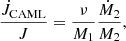$\begin{matrix} \frac{{\dot{J}}_{CAML}}{J} = \frac{ν}{M_{1}} \frac{{\dot{M}}_{2}}{M_{2}}, \end{matrix}$ $Mathematical equation: $$ \begin{aligned} \frac{\dot{J}_{\mathrm{CAML} }}{J} = \frac{\nu }{M_1}\frac{\dot{M}_2}{M_2}, \end{aligned} $$$ (7)

where J is the total orbital angular momentum and ν = 0.35 M_⊙. This prescription is now commonly adopted in CV evolution studies because it offers a practical solution to the WD mass problem (e.g. Belloni et al. 2018), although its underlying physical mechanism remains unknown (Zorotovic & Schreiber 2020; Tang et al. 2024).

3. Convective turnover time from stellar structure

3.1. Impact on MB torque and CV evolution

Equations (2) and (3) show that the convective turnover time, τ_c, is a key parameter for MB in the saturated regime, with ${\dot{J}}_{MB, SAT} \propto τ_{c}^{- 2}$ $Mathematical equation: $ \dot{J}_{\mathrm{MB, SAT}}\propto\tau_c^{-2} $$ . Previous SBD MB studies have adopted the smooth, mass-only empirical relation τ_c(M) from Wright et al. (2011). This prescription is potentially unreliable for fully convective low-mass M dwarfs, where observational constraints are sparse (Wright et al. 2018; Magaudda et al. 2020). Moreover, empirical τ_c relations derived from single stars may not apply directly to mass-losing donors in CVs. Recently, Gossage et al. (2025) found, both empirically and theoretically, a sharp increase in τ_c near 0.35 M_⊙, where typical M dwarfs become fully convective. This motivates the idea that the MB torque can change abruptly at the fully convective boundary. For example, a ∼5× increase in τ_c is sufficient to produce the desired disruption factor η ∼ 25.

We followed the approach of Gossage et al. (2025)² in the calculation of τ_c from the stellar structure using MESA. Physically, τ_c characterises the timescale of convective motions in the stellar interior. The size and velocity of convective cells vary with depth, and within mixing-length theory τ_c can be defined locally as (e.g. Brandenburg & Subramanian 2005)

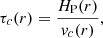$\begin{matrix} τ_{c} (r) = \frac{H_{P} (r)}{v_{c} (r)}, \end{matrix}$ $Mathematical equation: $$ \begin{aligned} \tau _c(r) = \frac{H_{\mathrm{P} }(r)}{v_c(r)}, \end{aligned} $$$ (8)

where H_P(r) = P(r)/g(r)ρ(r) is the local pressure scale height, and v_c(r) is the local convective velocity. Magnetic dynamos are believed to operate near the base of the convective envelope, at the interface with the radiative core, in a thin shear layer known as the tachocline (Parker 1955, 1975; Spiegel & Zahn 1992). This motivates evaluating τ_c near the base of the convective envelope r_BCE. However, as the star becomes fully convective, r_BCE matches its centre and divergence would occur as g(r_BCE → 0)→0 and v_c(r_BCE → 0)→0. A practical solution is to evaluate τ_c at some distance from the bottom of the convective envelope. For example, Gilliland (1985) proposed using one scale height above (r = r_BCE + H_P(r_BCE)), and Gossage et al. (2025) adopted half a local scale height above (r = r_BCE + 0.5H_P(r_BCE)). We decided to use one scale height above as it reproduces the empirical relation of Wright et al. (2011) at M ≳ 0.5 M_⊙.

The results of incorporating the new structure-based τ_c into the SBD MB model for CV evolution are shown in Fig. 1. For comparison, we also show the empirical SBD MB with K = η = 30 (Barraza-Jorquera et al. 2025). Upper panels show the mass transfer rate Ṁ versus orbital period P_orb and donor radius R₂ versus mass M₂. The lower right panel shows the τ_c − M₂ relation for the simulations using new τ_c calculation compared with the empirical τ_c(M) relation of Wright et al. (2011) used in previous studies. For the models with new τ_c calculation, η is calculated simply as η = (τ_c^calc/τ_c^emp)², where τ_c^emp is given by the empirical relation of Wright et al. (2011). The structure-based τ_c broadly agree with the empirical relation at M₂ ≳ 0.5 M_⊙. In typical M dwarfs, the fully convective boundary corresponds to M ≈ 0.35 M_⊙ (Chabrier & Baraffe 1997). In the case of CV donors, the fully convective boundary is shifted to lower masses M₂ ≈ 0.2 − 0.25 M_⊙. Our simulations show a spike in τ_c at M₂ ≈ 0.25 M_⊙ corresponding to a ∼2 − 3× increase. This spike directly triggers a quick MB disruption by a factor of η ∼ 5, and the system naturally detaches, entering the period gap. Because the τ_c values are systematically larger than the empirical ones for M₂ ≲ 0.5 M_⊙, we found that a stronger boosting factor K = 50 is needed above the gap. However, the system then re-establishes contact too early and the post-gap accretion rates are too high, indicating that the effective boost must drop once detachment occurs. We therefore reduced the boost when the system detaches (for example when Ṁ ≲ 10⁻²⁰ M_⊙ yr⁻¹) and found that a residual value K₂ = 2 works well. The lower left panel of Fig. 1 shows the evolution of the convective and radiative regions and the resulting τ_c(P_orb) for the two-stage K₁ → K₂ model. As the radiative core shrinks and the convective envelope deepens towards full convection, the locally evaluated τ_c increases.

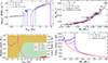Fig. 1.

CV evolution models that use the SBD MB prescription with the convective turnover time (τ_c) computed directly from the donor structure. Upper left: Mass transfer rate (Ṁ) versus orbital period (P_orb). Upper right: Donor radius (R₂) versus donor mass (M₂). Grey star symbols show observational determinations from McAllister et al. (2019), and the red line is the semi-empirical donor sequence of Knigge et al. (2011). For comparison, the empirical SBD MB model with K = η = 30 (Barraza-Jorquera et al. 2025) is shown, in green. The blue track adopts the same constant boost, K = 30. The magenta track uses a two-stage boost, transitioning from K₁ = 50 above the gap to K₂ = 2 once the system detaches and enters the gap. Lower left: Evolution of the convective and radiative regions and the resulting τ_c(P_orb) for the two-stage model. Lower right: τ_c − M₂ relation for the two simulations using the new τ_c calculation compared with the empirical τ_c(M) relation from Wright et al. (2011). A pronounced spike in τ_c appears when the donor becomes fully convective.

We note that the present model involves some circularity. By assuming that the relevant dynamo operates near the interface between the convective envelope and the radiative core, the weakening of MB is naturally linked to the disappearance of that interface as the donor approaches full convection. In this sense, the MB disruption is built into the adopted physical picture. At present, the precise role of the tachocline in dynamos of low-mass stars, and the relation between partially and fully convective dynamos remain uncertain (Guerrero et al. 2016; Wright et al. 2018; Käpylä et al. 2023; Lu et al. 2024). This leaves room for alternative assumptions about the dynamo-relevant region and the most appropriate definition of τ_c.

3.2. Dependence on the τ_c definition

To assess how strongly our results depend on the adopted definition of τ_c, we repeated the simulations using different prescriptions for τ_c. In addition to our adopted local prescription evaluated at r = r_BCE + H_P(r_BCE), we considered the alternative local prescription of Gossage et al. (2025), evaluated at r = r_BCE + 0.5H_P(r_BCE), as well as the global envelope-integrated definition:

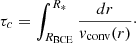$\begin{matrix} τ_{c} = \int_{R_{BCE}}^{R_{*}} \frac{dr}{v_{conv} (r)} \cdot \end{matrix}$ $Mathematical equation: $$ \begin{aligned} \tau _c = \int _{R_{\mathrm{BCE} }}^{R_*} \frac{dr}{v_{\mathrm{conv} }(r)}\cdot \end{aligned} $$$ (9)

This definition has, for example, been adopted in the convection and rotation-boosted MB prescription of Van & Ivanova (2019)³ and in the recent recalibration of SBD MB by Barraza-Jorquera et al. (2026)⁴. Unlike the local prescriptions, the global definition does not assume the tachocline to be the unique dynamo-relevant location. Therefore, it has the conceptual advantage that the increase in τ_c emerges from the structure of the entire convective envelope.

Figure 2 compares CV evolutionary tracks computed with these three τ_c prescriptions. For each case, we allowed the MB boost parameters to be adjusted so as to preserve a broadly consistent CV evolutionary picture, including the period gap and period minimum. To illustrate the behaviour over a wider mass range, we used an initial donor mass of 1 M_⊙. The figure also compares the resulting τ_c − M₂ relations with the empirical relation of Wright et al. (2011) and the updated relation from Wright et al. (2018). Most importantly, all three prescriptions show a pronounced increase in τ_c as the donor approaches the fully convective boundary at M₂ ≈ 0.25 M_⊙. The relative amplitude of this feature is very similar in all cases, corresponding to a ∼2 − 3× increase compared to the values immediately above the transition. The main difference between the prescriptions lies instead in the overall normalisation of τ_c. The local prescription evaluated at r = r_BCE + H_P remains close to the empirical τ_c − M relation of Wright et al. (2011), while the alternative local prescription at r = r_BCE + 0.5H_P is more consistent with the updated relation from Wright et al. (2018). By contrast, the global envelope-integrated definition yields systematically larger values of τ_c, likely reflecting the different averaging procedure rather than the same physical timescale being measured. As a result, in our calibration the global definition requires MB boost factors roughly an order of magnitude larger than the adopted local prescription evaluated at r = r_BCE + H_P in order to reproduce similar CV evolutionary tracks.

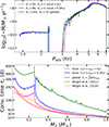Fig. 2.

Sensitivity of the CV evolution and the τ_c − M₂ relation to the adopted convective turnover time prescription. For each case, the boost factors K₁ and K₂ were adjusted to preserve broadly consistent CV evolutionary tracks. The corresponding τ_c − M₂ relations are compared with the empirical relations of Wright et al. (2011) and Wright et al. (2018). All three prescriptions produce a pronounced increase in τ_c near the fully convective boundary with similar amplitudes, although normalisation depends on the adopted definition.

Taken together, this analysis indicates that the initial MB disruption by a factor of η ∼ 5 is robust across the different τ_c prescriptions explored here, and is primarily driven by the spike in τ_c. The CV period gap is initiated by the donor’s structural response as it approaches full convection. The subsequent reduction of the boost below the gap suggests that the boosting mechanism should also depend on the donor’s structure. In the remainder of this paper, we adopt the local definition evaluated at r = r_BCE + H_P, as it allows direct comparisons with previous SBD MB studies.

4. Donor irradiation by the accreting WD

We used a simplified model to assess whether irradiation-driven winds in CVs can produce a significant enhancement of MB and thereby account for the empirical boost factor (K). We note that irradiation is an inherently anisotropic process that cannot be modelled explicitly in a 1D stellar structure code. The solution is to approximate it as an effective, spherically averaged heat source deposited in the donor’s outer envelope, which is appropriate for studying secular evolution.

4.1. The irradiation model

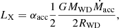
We computed the X-ray luminosity assuming that half of the gravitational energy of the accreted matter is released in the hot boundary layer, which generates X-rays (see e.g. Patterson & Raymond 1985; Rodriguez et al. 2025):

$\begin{matrix} L_{X} = α_{acc} \frac{1}{2} \frac{G M_{WD} {\dot{M}}_{acc}}{2 R_{WD}}, \end{matrix}$ $Mathematical equation: $$ \begin{aligned} L_{\mathrm{X} } = \alpha _{\mathrm{acc} }\frac{1}{2}\frac{G M_{\mathrm{WD} } \dot{M}_{\mathrm{acc} }}{2R_{\mathrm{WD} }}, \end{aligned} $$$ (10)

where α_acc is the radiative efficiency of accretion, M_WD and R_WD are the WD mass and radius, and Ṁ_acc is the mass accretion rate. The additional factor of 1/2 reflects the assumption that only half of the boundary-layer X-ray emission escapes outwards, while the other half is intercepted and absorbed by the WD. For a given WD mass, we computed R_WD from the zero-temperature WD mass–radius relation of Nauenberg (1972). The accretion efficiency (α_acc) is an unknown parameter that we tried to relate to realistic values from observations. Rodriguez et al. (2025) obtained that α_acc = 0.02 − 0.3 can adequately reproduce the observed X-ray luminosities of the CV population.

To compute the amount of X-ray luminosity L_X absorbed by the donor, we adopted the point–source irradiation model (King et al. 1996; Ritter et al. 2000; Büning & Ritter 2004). In this model, the accreting WD is treated as an isotropic point source at separation a. The local irradiating flux on a surface element depends on its orientation and position on the donor star. For a surface element at colatitude θ, the irradiating flux normal to the surface can be written as

$\begin{matrix} F_{X, irr} (θ) = α_{irr} \frac{L_{X}}{4 π a^{2}} h (θ), \end{matrix}$ $Mathematical equation: $$ \begin{aligned} F_{\rm X, irr}(\theta ) = \alpha _{\mathrm{irr} }\frac{L_{\rm X}}{4\pi a^2}h(\theta ), \end{aligned} $$$ (11)

where α_irr is an irradiation efficiency that accounts for disc shadowing and the donor’s albedo, and h(θ) is the geometrical factor (see e.g. Büning & Ritter 2004 for an illustration):

$\begin{matrix} h (θ) = \frac{cos (θ) - cos (θ_{\max})}{{(1 - 2 cos (θ) cos (θ_{\max}) + {cos}^{2} (θ_{\max}))}^{3 / 2}}, \end{matrix}$ $Mathematical equation: $$ \begin{aligned} h(\theta ) = \frac{\cos (\theta )-\cos (\theta _{\rm max})}{(1-2\cos (\theta )\cos (\theta _{\rm max})+\cos ^2(\theta _{\rm max}))^{3/2}}, \end{aligned} $$$ (12)

where θ_max = arccos(R₂/a) is the maximum colatitude for direct irradiation. Integrating F_X, irr(θ) over the illuminated (day-side) surface of the donor yields the total power absorbed by the donor:

$\begin{matrix} P_{abs} = \int_{day} F_{X, irr} (θ) d A = α_{irr} \frac{L_{X}}{4 π a^{2}} \int_{0}^{2 π} \int_{0}^{θ_{\max}} h (θ) R_{2}^{2} sin (θ) d ϕ d θ . \end{matrix}$ $Mathematical equation: $$ \begin{aligned} P_{\rm abs} = \int _{\rm day} F_{\rm X, irr}(\theta ) \mathrm{d}A = \alpha _{\mathrm{irr} }\frac{L_{\rm X}}{4\pi a^2}\int _0^{2\pi }\int _0^{\theta _{\rm max}}h(\theta )R_2^2 \sin (\theta )\,\mathrm{d}\phi \,\mathrm{d}\theta . \end{aligned} $$$ (13)

The integral can be evaluated to give the final formula accounting for the geometry:

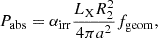$\begin{matrix} P_{abs} = α_{irr} \frac{L_{X} R_{2}^{2}}{4 π a^{2}} f_{geom}, \end{matrix}$ $Mathematical equation: $$ \begin{aligned} P_{\rm abs} = \alpha _{\mathrm{irr} }\frac{L_{\rm X}R_2^2}{4\pi a^2}f_{\rm geom}, \end{aligned} $$$ (14)

with the geometrical factor given by

$\begin{matrix} f_{geom} = 2 π \frac{1 - \sqrt{1 - {(R_{2} / a)}^{2}}}{{(R_{2} / a)}^{2}} \cdot \end{matrix}$ $Mathematical equation: $$ \begin{aligned} f_{\rm geom} = 2\pi \frac{1-\sqrt{1-(R_2/a)^2}}{(R_2/a)^2}\cdot \end{aligned} $$$ (15)

In the limit R₂/a ≪ 1, one recovers f_geom → π, and P_abs reduces to the familiar projected–area expression P_abs = α_irrL_X(R₂²/4a²). For typical CV parameters, we find that the geometrical factor induces only a modest < 10% difference compared to the simple projected-area expression. The irradiation efficiency α_irr is our second unknown parameter, in addition to α_acc. In the idealised case where the accretion disc lies exactly in the orbital plane and does not obscure the line between the WD and the donor, disc shadowing becomes negligible and the efficiency reduces to α_irr ≈ (1 − A_X). Here, A_X is the X-ray albedo of the donor describing how much of the incident X-ray flux is reflected. Several studies of X-ray illuminated stellar atmospheres show that at most ∼30 − 50% of the X-ray flux could be reflected (Basko et al. 1974; Felsteiner & Opher 1976; London et al. 1981). Therefore, the irradiation efficiency should be about α_irr ≳ 0.5.

We deposited P_abs as an additional, spherically averaged heat source in the donor’s outer envelope. We parametrised the deposition depth by the column depth (Σ):

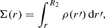$\begin{matrix} Σ (r) = \int_{r}^{R_{2}} ρ (r') d r', \end{matrix}$ $Mathematical equation: $$ \begin{aligned} \Sigma (r) = \int _r^{R_2} \rho (r\prime )\,\mathrm{d}r\prime , \end{aligned} $$$ (16)

which describes the mass per unit surface area above radius r. In discretised form, the column depth at the outer face of zone k is obtained by summing inwards from the surface:

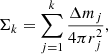$\begin{matrix} Σ_{k} = \sum_{j = 1}^{k} \frac{Δ m_{j}}{4 π r_{j}^{2}}, \end{matrix}$ $Mathematical equation: $$ \begin{aligned} \Sigma _k = \sum _{j = 1}^{k}\frac{\Delta m_j}{4\pi r_j^2}, \end{aligned} $$$ (17)

where Δm_j is the mass of zone j and r_j is the representative shell radius. By default, MESA deposits the additional heating uniformly down to a prescribed column depth (with the standard choice Σ = 1 g cm⁻²). Instead, we adopted an exponential deposition law:

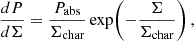$\begin{matrix} \frac{dP}{d Σ} = \frac{P_{abs}}{Σ_{char}} exp (- \frac{Σ}{Σ_{char}}), \end{matrix}$ $Mathematical equation: $$ \begin{aligned} \frac{dP}{d\Sigma }=\frac{P_{\rm abs}}{\Sigma _{\rm char}} \exp \!\left(-\frac{\Sigma }{\Sigma _{\rm char}}\right), \end{aligned} $$$ (18)

where Σ_char is the characteristic column depth that controls how concentrated the heating is towards the near-surface layers. In principle, a more realistic treatment would account for the incident X-ray spectrum and assign energy-dependent penetration depths (Quintin & Nelson 2013)⁵. A full spectral treatment is beyond the scope of this study and we adopted Σ_char = 3 g cm⁻². We verified that varying this parameter over the range Σ_char = 1 − 30 g cm⁻² leaves the evolutionary tracks largely unchanged. For smaller values, the stronger concentration of heating in the outermost layers can occasionally trigger unstable mass transfer under strong irradiation. For a zone bounded by Σ_k − 1 and Σ_k, the deposited power is

$\begin{matrix} Δ P_{k} & = P_{abs} [exp (- \frac{Σ_{k - 1}}{Σ_{char}}) - exp (- \frac{Σ_{k}}{Σ_{char}})] \end{matrix}$ $Mathematical equation: $$ \begin{aligned} \Delta P_k&= P_{\rm abs}\left[\exp \!\left(-\frac{\Sigma _{k-1}}{\Sigma _{\rm char}}\right) -\exp \!\left(-\frac{\Sigma _{k}}{\Sigma _{\rm char}}\right)\right] \end{aligned} $$$ (19)

$\begin{matrix} = P_{abs} exp (- \frac{Σ_{k - 1}}{Σ_{char}}) [1 - exp (- \frac{Δ Σ_{k}}{Σ_{char}})], \end{matrix}$ $Mathematical equation: $$ \begin{aligned}&= P_{\rm abs}\,\exp \!\left(-\frac{\Sigma _{k-1}}{\Sigma _{\rm char}}\right) \left[1-\exp \!\left(-\frac{\Delta \Sigma _k}{\Sigma _{\rm char}}\right)\right], \end{aligned} $$$ (20)

which guarantees the correct normalisation ∑_kΔP_k ≃ P_abs. We converted ΔP_k to a specific heating rate,

$\begin{matrix} ϵ_{k} = \frac{Δ P_{k}}{Δ m_{k}}, \end{matrix}$ $Mathematical equation: $$ \begin{aligned} \epsilon _k = \frac{\Delta P_k}{\Delta m_k}, \end{aligned} $$$ (21)

and injected it into the stellar energy equation via MESA’s per-cell extra-heating term (extra_heat). We prefer the exponential profile as given by Eq. (18) because irradiation is expected to be absorbed predominantly in the upper layers, and a uniform-cutoff prescription introduces a sharp discontinuity at the base of the heated region that can lead to numerical instabilities.

We considered an additional donor wind component that is induced by irradiation heating. The motivation is that if the energy deposited by irradiation in the donor’s outer layers is sufficient to raise the local temperature and drive expansion, an extra outflow may be launched from the irradiated hemisphere. We treated this process in a highly simplified, energy-limited way and did not attempt to model the full hydrodynamics of wind generation. In general, the wind dynamics depend on hydrodynamical properties of the heating and cooling regimes, as well as the incident X-ray spectrum of irradiation (Basko et al. 1977; Ruderman et al. 1989; Tavani & London 1993). To lift material from the stellar surface out of the donor’s potential well, the minimum required specific energy is of order the escape energy E_esc ≈ GM₂/R₂. Since only a fraction of the irradiation-induced energy can be converted into mechanical work (with the rest radiated away), a wind efficiency coefficient α_wind must be introduced. Comparing the available driving power (α_windP_abs) with the mechanical power carried by the wind (Ṁ_wind,irr E_esc), we obtained

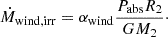$\begin{matrix} {\dot{M}}_{wind, irr} = α_{wind} \frac{P_{abs} R_{2}}{G M_{2}} \cdot \end{matrix}$ $Mathematical equation: $$ \begin{aligned} \dot{M}_{\rm wind,irr} = \alpha _{\mathrm{wind} }\frac{P_{\rm abs}R_2}{GM_2}\cdot \end{aligned} $$$ (22)

It is believed that α_wind is a relatively small parameter. Tavani & London (1993) estimated α_wind ∼ 10⁻¹ − 10⁻³ in LMXBs from hydrodynamical calculations. Justham et al. (2006) and Chen & Podsiadlowski (2016) used α_wind ∼ 10⁻³ − 10⁻⁵ to simulate the evolution of compact X-ray binaries with black holes and neutron stars. Xing & Li (2019) also used α_wind ∼ 10⁻² − 10⁻³ to explain the formation of the compact binary 2A 1822−371. We found that for typical CV parameters and plausible efficiencies, the irradiation-driven wind loss is typically of order Ṁ_wind,irr ≲ 10⁻¹¹ M_⊙ yr⁻¹. The impact of this extra mass loss on the mass-transfer budget is small compared to the accretion-driven mass-transfer rate but the irradiation-driven wind can still be a significant fractional enhancement relative to the donor’s intrinsic (base) wind Ṁ_wind,base, and may therefore produce a substantial boost of the MB torque. To express this MB boosting, we compared the irradiation-induced wind to the base wind:

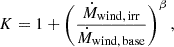$\begin{matrix} K = 1 + {(\frac{{\dot{M}}_{wind, irr}}{{\dot{M}}_{wind, base}})}^{β}, \end{matrix}$ $Mathematical equation: $$ \begin{aligned} K = 1+ \left(\frac{\dot{M}_{\rm wind,\,irr}}{\dot{M}_{\rm wind,\,base}}\right)^{\beta }, \end{aligned} $$$ (23)

where β describes how the MB torque scales with wind mass loss ${\dot{J}}_{MB} \propto {\dot{M}}_{wind}^{β}$ $Mathematical equation: $ \dot{J}_{\mathrm{MB}}\propto \dot{M}_{\mathrm{wind}}^\beta $$ ⁶. In modern MB formulations the dependence of torque on other parameters is expressed through an exponent m, which relates to our parameter as β = 1 − 2m (Matt et al. 2015). Magnetohydrodynamic simulations suggest that m is determined primarily by the magnetic field geometry and wind acceleration profile, and likely m ∼ 0.2 − 0.25 (Réville et al. 2015). Therefore, β is expected to be of order β ∼ 0.5.

Unfortunately, the base wind mass-loss rates of M dwarfs (Ṁ_wind,base) remain poorly constrained. Wood et al. (2021) report estimates for 17 M dwarfs and find that almost all of them satisfy Ṁ_wind,base ≲ Ṁ_⊙ (see also Walters et al. 2023). Although there exist prescriptions that relate wind mass-loss rates to stellar parameters (e.g. Reimers 1975; de Jager et al. 1988; Schröder & Cuntz 2005; Johnstone et al. 2015a), these relations are highly uncertain for low-mass M dwarfs, particularly near the fully convective boundary. In our case, we found that such prescriptions can also be inconsistent with empirical upper limits (Wood et al. 2021; Walters et al. 2023). We therefore adopted the simplification of a constant base wind in all simulations:

$\begin{matrix} {\dot{M}}_{wind, base} = 0.1 {\dot{M}}_{⊙}, \end{matrix}$ $Mathematical equation: $$ \begin{aligned} \dot{M}_{\rm wind,\,base } = 0.1\,\dot{M}_\odot , \end{aligned} $$$ (24)

where for the solar wind mass-loss rate we used Ṁ_⊙ = 1.4 × 10⁻¹⁴ M_⊙ yr⁻¹ (Johnstone et al. 2015b). We note that this ad hoc choice mainly affects the normalisation of the MB boost (K). For alternative values of Ṁ_wind,base, the desired K can still be obtained by varying the uncertain efficiency factors α_acc, α_irr, and α_wind. In practice, the value adopted in Eq. (24) allows these efficiencies to remain within the plausible bounds discussed above.

4.2. Mass-transfer cycles

The irradiation prescription above couples the instantaneous mass-transfer rate Ṁ_acc to the donor structure and to the MB torque. Because accretion rate responds extremely sensitively to small changes in the degree of overfill (see Eq. 5), these couplings form a stiff feedback that can naturally produce relaxation oscillations (mass-transfer cycles). Irradiation-driven cycles have previously been found even when irradiation affects the donor only through heating and flux blocking, without any additional wind-driven MB enhancement (e.g. Ritter et al. 2000; Büning & Ritter 2004). In our framework, the same structural feedback is present, but irradiation also drives an additional wind component that boosts the MB torque, introducing a second positive feedback loop. Figure 3 summarises the two loops.

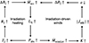Fig. 3.

Schematic diagram of the two positive feedback loops in our irradiation model that make the mass-transfer response stiff and result in mass-transfer cycles. An increase in the accretion rate (Ṁ_acc) raises the accretion luminosity (L_X) and the absorbed irradiation power (P_abs). In the heating loop (left), irradiation modifies the donor’s outer boundary conditions, driving expansion (R₂↑), which increases the Roche lobe overfill ΔR₂ ≡ R₂ − R_2, R and hence further enhances Ṁ_acc (see Eq. 5). In the wind loop (right), irradiation drives a wind Ṁ_wind,irr that increases the MB boost factor (K) and the MB torque ( $| {\dot{J}}_{MB} |$ $Mathematical equation: $ |\dot{J}_{\mathrm{MB}}| $$ ), shrinking the orbit and Roche lobe (R_2, R↓), again increasing ΔR₂ and Ṁ_acc.

Figure 4 shows an example of mass-transfer cycles for a representative model with α_acc = 0.1, α_irr = 0.75, α_wind = 0.001, β = 0.55. Immediately after the onset of mass transfer, the system exhibits low-amplitude oscillations without complete detachment. At later times the cycles occur more rarely and the variability becomes more pronounced with Ṁ jumping from ≲10⁻²⁰ to ∼10⁻⁸ M_⊙ yr⁻¹. After ≈600 Myr, Ṁ rises to ≳10⁻⁶ M_⊙ yr⁻¹ and the evolution becomes unstable. The zoomed-in plots show the morphology of individual cycles with the system spending only a small fraction of each cycle near the peak Ṁ. The characteristic period of such cycles is set by the thermal adjustment of the donor’s outer envelope and is therefore of order a few million years (see the bottom panel of Fig. 4). Such timescales are far longer than the ∼century observational baseline, so direct detection of a cycle in a single object is not feasible. Nevertheless, if large-amplitude cycles of this kind were common, a population observed at random phases would exhibit substantial scatter in inferred Ṁ, which is not seen in CVs. This suggests that strong irradiation-driven mass-transfer cycles are unlikely to occur in real CVs, although more detailed simulations are required to robustly assess their plausibility.

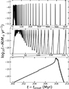Fig. 4.

Mass-transfer rate as a function of time since the onset of mass transfer for the irradiated model (see the main text for details). The evolution exhibits recurrent mass-transfer cycles. After ≈600 Myr, Ṁ rises to ≳10⁻⁶ M_⊙ yr⁻¹ and the simulation terminates. The middle and bottom panels show successive zoom-ins of the time intervals highlighted. The markers in the bottom panel indicate the discrete simulation steps, illustrating the temporal resolution across the cycle.

4.3. Smoothing on a characteristic timescale

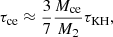
We tried suppressing the rapid irradiation response by applying temporal smoothing to the absorbed irradiation power on the characteristic thermal timescale of the donor’s convective envelope. For a chemically homogeneous star, the convective-envelope timescale can be approximated by (see Eq. (66) in Büning & Ritter 2004):

$\begin{matrix} τ_{ce} \approx \frac{3}{7} \frac{M_{ce}}{M_{2}} τ_{KH}, \end{matrix}$ $Mathematical equation: $$ \begin{aligned} \tau _{\rm ce} \approx \frac{3}{7}\frac{M_{\rm ce}}{M_2}\tau _{\rm KH}, \end{aligned} $$$ (25)

where τ_KH = GM₂²/R₂L₂ is the donor’s Kelvin-Helmholtz thermal timescale, and M_ce is the mass of the convective envelope. We compared the evolution timestep (dt) with τ_ce and damped the irradiation response by updating the absorbed power only partially each step:

$\begin{matrix} P_{abs}^{i} = P_{abs}^{i - 1} + f (P_{abs}^{inst} - P_{abs}^{i - 1}), \end{matrix}$ $Mathematical equation: $$ \begin{aligned} P_{\rm abs}^i = P_{\rm abs}^{i-1} + f(P_{\rm abs}^\mathrm{inst}-P_{\rm abs}^{i-1}), \end{aligned} $$$ (26)

where f ≡ dt/τ_ce is the smoothing factor, $P_{abs}^{i - 1}$ $Mathematical equation: $ P_{\mathrm{abs}}^{i-1} $$ is the absorbed irradiation power from the previous simulation step, and $P_{abs}^{inst}$ $Mathematical equation: $ P_{\mathrm{abs}}^{\mathrm{inst}} $$ is the instantaneous absorbed power calculated from Eq. (14). In practice, we took f = min(1, dt/τ_ce) so that 0 ≤ f ≤ 1 for all timesteps. This approach allowed us to completely suppress mass-transfer cycles as typically during accretion dt ≪ τ_ce and the smoothing is strong with f ≲ 0.01, so P_abs changes by at most ≲1% per timestep. We stress that this is an ad hoc smoothing prescription. While the heating loop (Fig. 3) can plausibly be damped on the convective envelope timescale, it is unlikely that the wind loop should be slowed by the same mechanism and on a similarly long timescale.

5. Evolution with the iτSBD MB model

We refer to the combined SBD MB prescription in which the disruption is set by a structure-based τ_c calculation and the boost arises from irradiation-driven wind enhancement as the iτSBD MB model. In what follows, we adopted the temporal smoothing to suppress irradiation-induced mass-transfer cycles.

5.1. Main results

Figure 5 presents evolutionary tracks obtained with the iτSBD MB model. For comparison, we also show the structure-based τ_c model without irradiation (K₁ = 50, K₂ = 2) and empirical SBD MB (K = η = 30). For the irradiation component we used α_acc = 0.1, α_irr = 0.5, α_wind = 10⁻¹, and β = 0.40. Once the system detaches, we reduced the wind efficiency to α_wind = 10⁻⁴, analogous to the K₁ → K₂ transition applied in Fig. 1. The lower right panel in Fig. 5 shows how the ratio K/η changes with orbital period for the three models. The iτSBD MB model naturally gives the required boost and disruption factors close to the empirical line (K = η = 30; Barraza-Jorquera et al. 2025). It also brings the donor mass-radius track closer than all other models to the semi-empirical donor sequence of Knigge et al. (2011) because the donor is inflated from irradiation. Interestingly, the iτSBD MB model shows episodes of higher accretion rate in the 3−4 h range, which could be attributed to nova-like CVs (see Sect. 6.2).

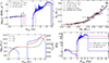Fig. 5.

CV evolution with the iτSBD MB model, including irradiation-driven winds and convective turnover times computed directly from the stellar structure. The adopted irradiation parameters are α_acc = 0.1, α_irr = 0.5, α_wind = 10⁻¹, and β = 0.40 (with α_wind reduced to 10⁻⁴ in the period gap). Upper panels: Same as Fig. 1 but with the smoothed iτSBD MB model added in blue. Lower left: Irradiation flux (F_irr; blue), donor global effective temperature (T_eff; green), and effective temperature of the irradiated hemisphere (T_irr; red) as functions of orbital period. Lower right: Ratio of the boost and disruption parameters (K/η) as a function of orbital period for the three models.

We also show on the lower left panel of Fig. 5 the irradiation flux, the donor’s global effective temperature, and the effective temperature of the irradiated hemisphere as functions of orbital period. We compute the irradiation flux as the total absorbed irradiation power distributed over the effectively irradiated surface F_irr = P_abs/(f_geomR₂²) (see also Eq. 14). The temperature of the irradiated region is then estimated by adding the irradiation flux to the donor’s intrinsic emergent flux, T_irr = (T_eff⁴ + F_irr/σ_SB)^1/4. The median temperature difference T_irr − T_eff is ≈250 K, while the maximum difference reaches ≈800 K at P_orb ≈ 5 h, when irradiation is strongest. As expected, the accretion-driven irradiation flux vanishes in the period gap and the temperatures equalise. Below the gap, F_irr increases towards shorter orbital periods as the binary separation decreases.

An important consequence of the iτSBD MB model, compared to the empirical SBD MB calibration, is the substantially longer evolutionary timescale. In iτSBD MB, the MB boost is tied to irradiation-driven winds and therefore operates only during phases of active accretion, so the post-common-envelope detached phase is long. By contrast, the empirical SBD MB prescription applies a constant boost (K = 30) from the very start, which accelerates orbital shrinkage and significantly shortens the time to contact (see also the lower right panel of Fig. 5). This difference is illustrated in Fig. 6: the empirical model reaches the onset of mass transfer at ≈170 Myr and terminates after ≈2.1 Gyr, whereas iτSBD MB reaches contact at ≈4.3 Gyr and terminates after ≈6.2 Gyr. Such differences may be important when confronting models with observables that depend on long-term thermal evolution of the WD. For example, the time to the onset of mass transfer should not be shorter than the typical WD pre-contact cooling time inferred for detached CV progenitors (Schreiber & Gänsicke 2003; Zorotovic et al. 2011a). It is also increasingly argued that the generation of strong magnetic fields in WDs requires timescales of order a few billion years (see Schreiber et al. 2021; Schreiber & Belloni 2025, and references therein). While the iτSBD MB sequence yields a comparatively long pre-contact time of t_onset ≈ 4.3 Gyr, it should be kept in mind that we adopted an initial orbital period of 1 d. The observed period distribution of post-common-envelope binaries suggests shorter periods about 0.5 d (Nebot Gómez-Morán et al. 2011; Zorotovic et al. 2011b), which would reduce t_onset in our model accordingly. Overall, the iτSBD MB timescales are therefore more consistent with expected CV formation ages.

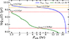Fig. 6.

Evolutionary age as a function of orbital period for the iτSBD MB model (blue) and the empirical SBD MB model with K = η = 30 (green). The dashed horizontal lines and annotations mark the time of first Roche lobe contact (t_onset) and the termination time of the calculation when M₂ < 0.05 M_⊙ (t_end).

5.2. Model behaviour for different parameters

Figure 7 shows simulations with the iτSBD MB model using different initial WD and donor masses. Overall, the evolutionary tracks are broadly consistent, showing small shifts in the period-gap boundaries and in the location of the period minimum. As a consequence of using eCAML, systems with low WD masses (M_WD ≲ 0.6 M_⊙) reach dynamically unstable mass transfer and are expected to merge (Schreiber et al. 2016). The simulation with M_WD = 0.7 M_⊙ also shows an atypical evolution, with the onset and end of the period gap occurring at longer periods than in the neighbouring models. Compared to the empirical SBD MB model (Barraza-Jorquera et al. 2025), the mass dependence is different because irradiation introduces an additional mass-dependent feedback on the secular evolution (see Eqs. 10, 14, and 22). It was emphasised before that the stability of irradiation prescriptions is sensitive to the assumed CAML strength (Ritter et al. 2000). This raises the possibility that irradiation may contribute to destabilising mass transfer even for weaker eCAML than assumed here. A detailed exploration of the interplay between irradiation feedback and CAML is beyond the scope of this work.

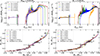Fig. 7.

Evolutionary tracks for different component masses using the iτSBD MB model. Ṁ versus P_orb (top row) and R₂ versus M₂ (bottom row). Left column: Tracks computed for fixed M_WD = 0.8 M_⊙ while varying the initial donor mass. Right column: Tracks computed for fixed M₂ = 0.8 M_⊙ while varying the initial WD mass. The blue curve corresponds to the fiducial model from Fig. 5. Other plot elements are the same as in Fig. 1.

The main uncertain parameters of the iτSBD MB model are the efficiency factors α_acc, α_irr, α_wind. In our framework, α_acc and α_irr are mathematically degenerate and therefore affect the secular evolution in the same way. Figure 8 shows the resulting changes in the evolutionary tracks in the Ṁ − P_orb plane when varying α_acc and α_wind. Since α_acc enters both the heating and wind feedback loops, whereas α_wind affects only the wind loop, the model is more sensitive to α_acc. For both too low and too high efficiencies, the system enters runaway mass transfer. For sufficiently low efficiencies, unstable mass transfer is triggered during an episode of enhanced Ṁ_acc as the donor approaches the fully convective boundary. For high efficiencies, the simulations show a phase of reversed orbital-period evolution around P_orb ≈ 5 h, in which the system widens and exhibits Ṗ > 0 in contrast to the usual Ṗ < 0. The model is even more sensitive to the exponent β that sets how the MB torque scales with the donor wind. Increasing it from β = 0.4 to β = 0.5 at fixed values of the other parameters is sufficient to drive the system into unstable mass transfer.

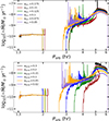Fig. 8.

Dependence of the iτSBD MB evolutionary tracks in the Ṁ − P_orb plane on model parameters. The top panel varies α_acc and the bottom panel varies α_wind, with all other parameters fixed. The blue curve corresponds to the fiducial model from Fig. 5.

6. Discussion

6.1. CV orbital period gap and minimum

An observational requirement for CV evolutionary models is to reproduce the orbital period gap and the period minimum. In the classical disrupted MB picture, the gap was explained by assuming that MB drops sharply once the donor becomes fully convective, causing the system to detach temporarily (Rappaport et al. 1983; Spruit & Ritter 1983). In practice, CV evolution above the gap is usually described with smooth MB prescriptions such as the RVJ law, while the disruption is set explicitly by sharply reducing or switching off MB once the donor becomes fully convective (Kolb 1993; Howell et al. 2001; Knigge et al. 2011; Belloni et al. 2018; Barraza-Jorquera et al. 2025). However, in this form the prescription is essentially phenomenological because the disruption is imposed by hand rather than emerging from the donor structure itself. Very few physically motivated prescriptions produce a period gap without such an ad hoc MB shutdown. One notable example is the double-dynamo model of Sarkar & Tout (2022). Our results suggest an alternative route in which the key trigger is the donor structure dependence of τ_c.

Our iτSBD MB model produces a gap in the canonical 2−3 h interval and a period minimum near ≈1.3 h = 78 min (see Fig. 5). To reproduce the mass-transfer rates below the period gap and the location of the period minimum our model requires an explicit change of the boost K across the gap (see Fig. 1). In our framework, the most plausible parameters for such a transition are the wind-related quantities α_wind and/or β, which are expected to depend on the donor’s magnetic field morphology. Physically, this may reflect a transition to a more complex magnetic topology as the donor crosses the fully convective boundary. Since the wind braking efficiency depends on the magnetic field morphology through the amount of open magnetic flux, more complex fields are expected to produce weaker AML (Réville et al. 2015; Garraffo et al. 2016, 2018). In this context, Barraza-Jorquera et al. (2026) found that in a different saturated MB formulation only a modest suppression of MB, by a factor of ∼2−3, is sufficient to reproduce the period gap. This suggests that the stronger disruption required in the original SBD MB framework may be partly overestimated by the underlying prescription, whereas our τ_c spike still naturally produces a moderate disruption of order η ∼ 5.

The period gap and minimum have been refined as larger and more homogeneous samples became available. Some of the widely adopted values place the period gap at 2.15−3.18 h, and the period minimum at 76−82 min (Knigge 2006; Gänsicke et al. 2009; McAllister et al. 2019). We tried to reproduce more accurately the observed period gap and period minimum (models 1 and 2 on Fig. 9)⁷. We adopted as a starting point the irradiation parameters α_acc = 0.1, α_irr = 0.5, α_wind = 10⁻¹ (reduced to 10⁻⁴ in the period gap), and β = 0.40. For model 1, we found that increasing β to 0.415 shifts the gap edges from 2−3 h to longer periods at ≈2.1 − 3.2 h. We then found that the initial orbital period also affects the width of the gap. For model 2, we used P_init = 0.725 d together with α_acc = 0.13, which provides a better match to the lower edge of the period gap.

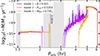Fig. 9.

Ṁ versus P_orb for the calibrated models used to reproduce the CV period gap and period minimum (see the main text for the model parameters). The approximate period minimum at 76−82 min and the period gap at 2.15−3.18 h are shown by the grey shaded regions (Knigge 2006). The vertical black line marks the recently revised lower edge of the period gap at 2.45 h (Schreiber et al. 2024). Models 1 and 2 were calibrated to match the classical gap, while model 3 shows that a lower initial WD mass of 0.7 M_⊙ helps reproduce the revised lower edge.

More recently, Schreiber et al. (2024) suggested a revised lower edge of the period gap at 2.45 h. In our models, the WD mass affects the location of this lower edge. As shown by model 3 in Fig. 9, an initial WD mass of 0.7 M_⊙ provides a better match to the revised value (see also Fig. 7). The Sloan Digital Sky Survey (SDSS) I–IV sample used by Schreiber et al. (2024) to infer the period gap edges is the largest homogeneous CV sample currently available (Inight et al. 2023). One possible interpretation is that the refined lower edge reflects the inclusion of systems hosting relatively low mass WDs, below the mean value of ⟨M_WD⟩≈0.8 M_⊙ (Zorotovic et al. 2011a; Pala et al. 2022). In this picture, our model suggests that the 2.15−2.45 h interval may be populated preferentially by CVs with lower mass WDs, which could now be revealed in the SDSS sample.

6.2. Implications for the accretion rates of nova-like CVs

Nova-like CVs are a subclass of CVs characterised by bright, persistently hot, and apparently stable accretion discs (Warner 2003; Puebla et al. 2007). In contrast to dwarf novae, nova-likes do not undergo disc-instability outbursts and instead sustain high accretion rates (Ṁ_acc ∼ 5 × 10⁻⁹ M_⊙ yr⁻¹) over long timescales (Dubus et al. 2018). Observationally, most known nova-likes reside above the period gap, with a strong concentration at P_orb ≃ 3 − 4 h, where they may account for up to ∼50% of the CV population (Rodríguez-Gil et al. 2007a). They are also among the strongest radio emitters in the CV population (Coppejans et al. 2015; Hewitt et al. 2020). The elevated accretion rates of nova-like CVs are difficult to reconcile with standard CV evolution models employing classical AML prescriptions (Gilmozzi & Selvelli 2024). Irradiation signatures have been observed in several nova-like CVs hosting very hot WDs, suggesting that irradiation may contribute to the unusually high mass-transfer rates in these systems (Araujo-Betancor et al. 2003; Rodríguez-Gil et al. 2007b).

Notably, our iτSBD MB model produces episodes of enhanced mass transfer in the same period range where nova-likes are most commonly found (Fig. 5). It is also clear that, across different initial conditions and model parameters, the full P_orb ∼ 3 − 4 h interval can be populated by CVs undergoing such high states, reaching peak accretion rates as high as Ṁ_acc ∼ 10⁻⁷ M_⊙ yr⁻¹ (see Figs. 7 and 8). These high-Ṁ_acc episodes coincide with changes in the donor’s convective structure. As the star evolves towards full convection, additional convective regions appear closer to the interior and the convective envelope adjusts in depth. Figure 10 illustrates this connection. When the convective envelope depth changes, the convective turnover time τ_c drops abruptly and the MB torque correspondingly increases. In physical terms, this behaviour may reflect a rapid reconfiguration of the large-scale magnetic field. We note that these enhanced Ṁ_acc episodes occur only in models that include irradiation (see Fig. 1 for comparison with a model without irradiation), indicating that irradiation plays an essential role in enabling these high states. Our simulations indicate that the typical duration of such enhanced Ṁ_acc episodes is of order ∼10⁵ yr and the recurrence time is ∼5× longer than the duration. Interestingly, during these enhanced Ṁ_acc episodes the model also exhibits positive Ṗ, with characteristic values Ṗ ∼ 10⁻¹². In classical MB prescriptions, sustained positive Ṗ is not achievable, whereas observations indicate that a substantial fraction of CVs display Ṗ > 0 (Schaefer 2024). Such short-baseline measurements do not necessarily imply deficiencies in standard AML prescriptions (King & Lasota 2021, 2024). Nevertheless, it is quite intriguing that our model naturally allows intervals of Ṗ > 0.

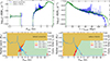Fig. 10.

Simulations with the iτSBD MB model illustrating episodes of enhanced mass transfer that may be associated with nova-like CVs. Upper left: Ṁ versus P_orb. Upper right: Ṁ versus time since the onset of mass transfer. Lower panels: Evolution of convective and radiative regions, together with the corresponding convective turnover time (τ_c), for the default convection with the Schwarzschild criterion (left) and the Ledoux criterion with additional mixing processes enabled (right).

We also explored the sensitivity of this behaviour to the convection prescription by adopting the Ledoux criterion (Ledoux 1947) and enabling semi-convection, thermohaline mixing, and convective overshooting⁸. In that case, the secondary convective regions form farther from the base of the convective envelope and have little impact on its depth, producing only modest Ṁ_acc fluctuations (see the right panels of Fig. 10). This suggests that enhanced mixing (probably overshooting) can weaken the high-Ṁ_acc episodes. However, choosing between the Schwarzschild and Ledoux criteria requires careful evaluation based on the stellar parameters (Canuto 2000; Gabriel et al. 2014). A more systematic exploration will be required to determine whether, and under what conditions, such enhanced Ṁ_acc episodes are possible.

6.3. Implications for stellar and binary evolution

The disruption of MB at the fully convective limit in low-mass stars is a stellar evolutionary feature, which has gained evidence from various sources. In CVs, MB disruption is directly observed as the fact of the existence of the period gap (Spruit & Ritter 1983). In post-common-envelope WD+MS binaries, the decrease in the number of systems at the fully convective limit provides evidence of MB disruption (Schreiber et al. 2010; Belloni et al. 2024; Zhou et al. 2026). A similar effect is also found in post-common-envelope hot subdwarf binaries (Blomberg et al. 2024). For single low-mass stars, rotation studies show that the spin-down timescale also increases towards masses below M₂ ≈ 0.35 M_⊙ (Delfosse et al. 1998; Reiners & Basri 2008; Irwin et al. 2011; Newton et al. 2016). However, recent studies of single stars in the vicinity of fully convective limit indicate additional complexity. An abrupt change in the spin-down law across the fully convective boundary is possible, with braking torques instead increasing there (Lu et al. 2024; Chiti et al. 2024). Our results suggest that low-mass stars rotating in the saturated MB regime should undergo a pronounced weakening of MB upon becoming fully convective, driven by the spike in τ_c.

Virtually all low-mass MS stars are expected to experience a pronounced increase in the convective turnover time τ_c at the fully convective boundary (Chiti et al. 2024; Gossage et al. 2025). In the SBD MB framework, which builds on the MB prescription of Chaboyer et al. (1995), this naturally results in MB disruption as ${\dot{J}}_{MB} \propto τ_{c}^{- 2}$ $Mathematical equation: $ \dot{J}_{\mathrm{MB}}\propto \tau_c^{-2} $$ in the saturated regime. However, this sensitivity to τ_c is not universal. For example, the widely used prescription of Matt et al. (2015), adopted by Barraza-Jorquera et al. (2026) in their revised SBD MB model, does not retain an explicit τ_c dependence in the saturated regime. Similarly, the convection and rotation-boosted prescription (Van et al. 2019; Van & Ivanova 2019), which has been applied successfully to LMXBs, yields ${\dot{J}}_{MB} \propto τ_{c}^{8 / 3}$ $Mathematical equation: $ \dot{J}_{\mathrm{MB}}\propto \tau_c^{8/3} $$ . Positive scalings, ${\dot{J}}_{MB} \propto τ_{c}^{n}$ $Mathematical equation: $ \dot{J}_{\mathrm{MB}}\propto \tau_c^{n} $$ with n > 0, typically arise when the surface magnetic field is assumed to scale with Rossby number B ∝ Ro⁻¹ ∝ τ_c/P_rot. Negative scalings such as ${\dot{J}}_{MB} \propto τ_{c}^{- 2}$ $Mathematical equation: $ \dot{J}_{\mathrm{MB}}\propto \tau_c^{-2} $$ are usually tied to saturated MB formulations in which the saturation threshold satisfies P_sat ∝ τ_c. Therefore, a spike in τ_c leads to MB disruption only in certain types of semi-empirical saturated MB prescriptions. A derivation of the MB torque that robustly predicts the saturated MB regime would therefore be highly valuable.

As shown in Sect. 5, our irradiation prescription can account for the enhanced MB required in CVs. The same physical mechanism should operate in other compact accreting binaries whose donors possess convective envelopes. Indeed, abnormally strong MB, interpreted as being driven by irradiation-induced winds, has been invoked to explain the evolution of several compact X-ray binaries (Justham et al. 2006; Chen & Podsiadlowski 2016; Xing & Li 2019; Zhao et al. 2026). Similar effects have also been proposed for spider pulsars, where strong irradiation of the companion can drive an ablated wind and enhance MB (Ginzburg & Quataert 2020, 2021; Conrad-Burton et al. 2023). Remarkably, Ginzburg & Quataert (2021) also found that a moderate reduction of MB at the fully convective transition best explains the observed spider sample, broadly consistent with the disruption of η ∼ 5 found here. This agreement between independent observational constraints supports the idea of a more universal physically motivated MB prescription.

A related question is whether irradiation-driven winds can also account for the MB boost inferred in detached binaries with hot primaries (Belloni et al. 2024; Blomberg et al. 2024). In detached systems, irradiation is easier to assess because it is not coupled to mass-transfer feedback. Although the incident spectrum differs from the accretion-powered irradiation considered for CVs, the same energy-limited framework can still be used for an order-of-magnitude estimate of the resulting donor wind, with the spectral differences most likely reflected in the uncertain efficiency parameters of the irradiation model. We therefore made simple estimates of the boost factor (K) expected in detached WD+MS and sdB+MS binaries by replacing the accretion-powered luminosity with the thermal luminosity of the primary, approximated as a blackbody by L₁ = 4πR₁²σ_SBT₁⁴. The corresponding MB boost in detached binaries can be written as (see Eqs. 14, 22, and 23)

$\begin{matrix} K \approx 1 + {(\frac{π α_{wind} α_{irr} σ_{SB} R_{1}^{2} T_{1}^{4} R_{2}^{3}}{G M_{2} a^{2} {\dot{M}}_{wind, base}})}^{β} . \end{matrix}$ $Mathematical equation: $$ \begin{aligned} K \approx 1 + \left(\frac{\pi \alpha _{\rm wind}\alpha _{\rm irr}\sigma _{\rm SB} R_1^2 T_1^4 R_2^3}{G M_2 a^2 \dot{M}_{\rm wind,base}}\right)^{\beta }. \end{aligned} $$$ (27)

For these estimates, we fixed the donor parameters at M₂ = 0.5 M_⊙ and R₂ = 0.5 R_⊙, since the empirical boost in detached systems appears to be most important for binaries with M₂ ≳ 0.4 M_⊙ (Belloni et al. 2024; Blomberg et al. 2024). We used M₁ = 0.6 M_⊙, R₁ = 0.012 R_⊙ and M₁ = 0.47 M_⊙, R₁ = 0.20 R_⊙ for systems with WD and sdB primaries, respectively. We also fixed α_irr = 0.7, β = 0.5, Ṁ_wind,base = 0.1 Ṁ_⊙, and P_orb = 0.5 d. We varied the poorly constrained wind efficiency between α_wind = 10⁻³ and 10⁻¹ in order to illustrate the possible spread in the resulting boost factor K arising from the current uncertainties in the parameters of the irradiation model. Table 1 summarises the resulting representative values of K for different temperatures of the primaries. These estimates suggest that the large boost K ≳ 50 inferred for post-common-envelope WD+M-dwarf binaries by Belloni et al. (2024) can be reached only if the WD is sufficiently hot (T₁ ≳ 30 000 K). By contrast, in sdB+MS binaries irradiation-driven winds can readily provide the required large boost K ≳ 100, as first proposed by Blomberg et al. (2024). This suggests that irradiation alone may be insufficient to explain the full MB boost in some detached binaries as WD+MS, and that an additional boosting mechanism may also be required in such systems. Irradiation-driven winds may also help explain the accretion rates in wind-fed magnetic systems such as low accretion rate polars, where the observed accretion rates of order 10⁻¹³ M_⊙ yr⁻¹ are difficult to reconcile with the weak intrinsic winds expected from M dwarfs (Webbink & Wickramasinghe 2005; Matranga et al. 2012) as well as some super soft X-ray sources like CAL 87, where the small mass ratio and expanding orbit deviate from the standard model for such sources (van Teeseling & King 1998; Ablimit & Li 2015).

Table 1.

Estimated irradiation-driven boost factors in detached binaries.

6.4. Model limitations and future work

While our iτSBD MB model provides a plausible route towards a physical interpretation of the empirical SBD boost and disruption, the present implementation still relies on several simplifying assumptions that should be addressed in future studies. One useful direction will be to investigate whether the physical ingredients proposed here can be incorporated into the revised SBD MB framework of Barraza-Jorquera et al. (2026).

The treatment of irradiation is highly idealised. The irradiation component introduces a number of uncertain parameters that are currently treated as constants, independent of system properties. In reality, the accretion efficiency (α_acc) should depend on the WD mass and radius, as well as on boundary-layer physics. The irradiation efficiency α_irr should depend on the incident spectrum, the donor’s atmospheric properties that determine the effective albedo, and possible shadowing by the accretion disc. The wind efficiency α_wind should depend on the hydrodynamics of wind launching. Also, together with the exponent β, they are expected to depend on the magnetic-field topology and wind-acceleration profile (Réville et al. 2015). A further simplification is our assumption of a constant base wind for the donor, Ṁ_wind,base = 0.1 Ṁ_⊙. A physically motivated prescription for wind mass-loss applicable to both partially and fully convective stars is clearly needed. In addition, we account only for irradiation associated with accretion and neglect direct irradiation by the hot WD itself. Such UV irradiation may also heat the donor significantly and could be especially important in detached systems with hot primaries.

Several additional ad hoc simplifications were adopted in the present CV evolution calculations. The need for temporal smoothing of P_abs to suppress irradiation-driven mass-transfer cycles indicates that the present treatment is incomplete. A more realistic approach should distinguish between the thermal response time of the donor’s outer envelope and the response time of the wind and MB torque to changes in irradiation. Another key limitation of the current model is that it still requires an explicit reduction of the MB boost once the system detaches and evolves below the gap. In practice, we mimic this by changing α_wind or β from a high to a low value within the gap. Although such a change is physically plausible, an important goal for future work is to replace these switches with a continuous and physically motivated prescription. Finally, several simplifying assumptions in the binary evolution setup were adopted. We kept the WD mass fixed, treated the WD as a point mass without thermal evolution, and adopted the eCAML prescription. In addition, including the suppression of MB via coupling between the donor and WD magnetospheres (Belloni et al. 2020) will allow us to extend the framework to magnetic CVs.

7. Conclusions

We have developed an extension of the empirical SBD MB model that incorporates irradiation-driven winds and convective turnover times computed directly from the stellar structure (the iτSBD MB model). We tested this prescription for CV evolution using MESA and found that:

Computing the convective turnover time (τ_c) directly from the donor structure produces a pronounced spike as the donor approaches full convection. In a saturated MB prescription ( ${\dot{J}}_{MB} \propto τ_{c}^{- 2}$ $Mathematical equation: $ \dot{J}_{\mathrm{MB}}\propto \tau_c^{-2} $$ ), this naturally yields a rapid reduction in the braking torque and can offer a physical explanation for MB disruption in CVs.
Accretion-powered irradiation can substantially modify the donor’s outer layers and strongly heat the donor-facing hemisphere. Irradiation-driven winds can enhance the effective MB torque during phases of active accretion and may provide a physical origin for the MB boost in CVs. The main limitation is that the present irradiation treatment remains highly simplified, relying on uncertain efficiencies, an assumed base wind for the M-dwarf donor, and ad hoc prescriptions for smoothing the irradiation response and for reducing the boost once the donor becomes fully convective.
Combining structure-based τ_c with irradiation-driven winds in the SBD MB framework yields evolutionary tracks that reproduce the main qualitative features of the CV population, including the period gap and period minimum. The model also brings the donor mass-radius relation closer to the semi-empirical donor sequence by allowing moderate donor inflation, predicts longer pre-contact evolutionary timescales that are more compatible with expected CV formation ages, and might produce episodic high-Ṁ_acc episodes in the 3−4 h range, where nova-like CVs are concentrated.

Overall, the iτSBD MB model provides a plausible physical interpretation of both the empirical boost and disruption factors and may be applicable to other close binaries with convective donors. The τ_c spike at the fully convective boundary offers a generic route to MB disruption in saturated-torque formulations, while irradiation-driven winds are expected to be relevant in compact binaries with sustained accretion and/or hot primaries. A key next step is to replace the present simplified irradiation prescription with a more physical treatment of wind launching and its coupling to the magnetic torque.

Data availability

The MESA code needed to reproduce the simulations presented in this work is available on Zenodo at https://zenodo.org/records/20201258

Acknowledgments

VD thanks Nanjing University for its hospitality during the visit and acknowledges support from Kazan Federal University. This work was supported by the National Key Research and Development Program of China (2021YFA0718500) and the Natural Science Foundation of China under grant numbers 12121003 and 12373034. IG and AS acknowledge support from Kazan Federal University. The authors thank the anonymous referee for their thoughtful review that helped significantly improve the manuscript.

References

Ablimit, I., & Li, X.-D. 2015, ApJ, 815, 17 [Google Scholar]
Andronov, N., Pinsonneault, M., & Sills, A. 2003, ApJ, 582, 358 [NASA ADS] [CrossRef] [Google Scholar]
Araujo-Betancor, S., Knigge, C., Long, K. S., et al. 2003, ApJ, 583, 437 [NASA ADS] [CrossRef] [Google Scholar]
Barnes, S. A. 2003, ApJ, 586, 464 [Google Scholar]
Barnes, S. A. 2007, ApJ, 669, 1167 [Google Scholar]
Barraza-Jorquera, J. A., Schreiber, M. R., & Belloni, D. 2025, A&A, 696, A92 [NASA ADS] [CrossRef] [EDP Sciences] [Google Scholar]
Barraza-Jorquera, J. A., Schreiber, M. R., Littlefair, S., Belloni, D., & Schwope, A. D. 2026, A&A, 708, L11 [NASA ADS] [CrossRef] [EDP Sciences] [Google Scholar]
Basko, M. M., & Sunyaev, R. A. 1973, Ap&SS, 23, 117 [Google Scholar]
Basko, M. M., Sunyaev, R. A., & Titarchuk, L. G. 1974, A&A, 31, 249 [NASA ADS] [Google Scholar]
Basko, M. M., Hatchett, S., McCray, R., & Sunyaev, R. A. 1977, ApJ, 215, 276 [Google Scholar]
Belloni, D., & Schreiber, M. R. 2023, Handbook of X-ray and Gamma-ray Astrophysics, 129 [Google Scholar]
Belloni, D., Schreiber, M. R., Zorotovic, M., et al. 2018, MNRAS, 478, 5626 [NASA ADS] [CrossRef] [Google Scholar]
Belloni, D., Schreiber, M. R., Pala, A. F., et al. 2020, MNRAS, 491, 5717 [Google Scholar]
Belloni, D., Schreiber, M. R., Moe, M., El-Badry, K., & Shen, K. J. 2024, A&A, 682, A33 [NASA ADS] [CrossRef] [EDP Sciences] [Google Scholar]
Blomberg, L., El-Badry, K., Breivik, K., et al. 2024, PASP, 136, 124201 [Google Scholar]
Brandenburg, A., & Subramanian, K. 2005, Phys. Rep., 417, 1 [NASA ADS] [CrossRef] [Google Scholar]
Büning, A., & Ritter, H. 2004, A&A, 423, 281 [NASA ADS] [CrossRef] [EDP Sciences] [Google Scholar]
Canuto, V. M. 2000, ApJ, 534, L113 [Google Scholar]
Chaboyer, B., Demarque, P., & Pinsonneault, M. H. 1995, ApJ, 441, 865 [Google Scholar]
Chabrier, G., & Baraffe, I. 1997, A&A, 327, 1039 [NASA ADS] [Google Scholar]
Chen, W.-C., & Podsiadlowski, P. 2016, ApJ, 830, 131 [CrossRef] [Google Scholar]
Chiti, F., van Saders, J. L., Heintz, T. M., et al. 2024, ApJ, 977, 15 [NASA ADS] [CrossRef] [Google Scholar]
Conrad-Burton, J., Shabi, A., & Ginzburg, S. 2023, MNRAS, 525, 2708 [NASA ADS] [Google Scholar]
Coppejans, D. L., Körding, E. G., Miller-Jones, J. C. A., et al. 2015, MNRAS, 451, 3801 [Google Scholar]
de Jager, C., Nieuwenhuijzen, H., & van der Hucht, K. A. 1988, A&AS, 72, 259 [NASA ADS] [Google Scholar]
Delfosse, X., Forveille, T., Perrier, C., & Mayor, M. 1998, A&A, 331, 581 [NASA ADS] [Google Scholar]
Deng, Z.-L., Li, X.-D., Gao, Z.-F., & Shao, Y. 2021, ApJ, 909, 174 [NASA ADS] [CrossRef] [Google Scholar]
Dubus, G., Otulakowska-Hypka, M., & Lasota, J.-P. 2018, A&A, 617, A26 [NASA ADS] [CrossRef] [EDP Sciences] [Google Scholar]
Eggleton, P. P. 1983, ApJ, 268, 368 [Google Scholar]
El-Badry, K., Conroy, C., Fuller, J., et al. 2022, MNRAS, 517, 4916 [NASA ADS] [CrossRef] [Google Scholar]
Fabry, M., & Prša, A. 2025, ApJ, 995, 19 [Google Scholar]
Felsteiner, J., & Opher, R. 1976, A&A, 46, 189 [Google Scholar]
Gabriel, M., Noels, A., Montalbán, J., & Miglio, A. 2014, A&A, 569, A63 [NASA ADS] [CrossRef] [EDP Sciences] [Google Scholar]
Galiullin, I., Rodriguez, A. C., El-Badry, K., et al. 2024, A&A, 690, A374 [NASA ADS] [CrossRef] [EDP Sciences] [Google Scholar]
Gänsicke, B. T., Dillon, M., Southworth, J., et al. 2009, MNRAS, 397, 2170 [NASA ADS] [CrossRef] [Google Scholar]
Garraffo, C., Drake, J. J., & Cohen, O. 2016, A&A, 595, A110 [NASA ADS] [CrossRef] [EDP Sciences] [Google Scholar]
Garraffo, C., Drake, J. J., Dotter, A., et al. 2018, ApJ, 862, 90 [NASA ADS] [CrossRef] [Google Scholar]
Gilliland, R. L. 1985, ApJ, 299, 286 [Google Scholar]
Gilmozzi, R., & Selvelli, P. 2024, A&A, 681, A83 [NASA ADS] [CrossRef] [EDP Sciences] [Google Scholar]
Ginzburg, S., & Quataert, E. 2020, MNRAS, 495, 3656 [Google Scholar]
Ginzburg, S., & Quataert, E. 2021, MNRAS, 500, 1592 [Google Scholar]
Gossage, S., Kalogera, V., & Sun, M. 2023, ApJ, 950, 27 [NASA ADS] [CrossRef] [Google Scholar]
Gossage, S., Kiman, R., Monsch, K., et al. 2025, ApJ, 988, 102 [Google Scholar]
Guerrero, G., Smolarkiewicz, P. K., de Gouveia Dal Pino, E. M., Kosovichev, A. G., & Mansour, N. N. 2016, ApJ, 819, 104 [NASA ADS] [CrossRef] [Google Scholar]
Hewitt, D. M., Pretorius, M. L., Woudt, P. A., et al. 2020, MNRAS, 496, 2542 [NASA ADS] [CrossRef] [Google Scholar]
Howell, S. B., Nelson, L. A., & Rappaport, S. 2001, ApJ, 550, 897 [Google Scholar]
Iben, I., Tutukov, A. V., & Fedorova, A. V. 1997, ApJ, 486, 955 [Google Scholar]
Inight, K., Gänsicke, B. T., Breedt, E., et al. 2023, MNRAS, 524, 4867 [NASA ADS] [CrossRef] [Google Scholar]
Irwin, J., Berta, Z. K., Burke, C. J., et al. 2011, ApJ, 727, 56 [Google Scholar]
Jermyn, A. S., Bauer, E. B., Schwab, J., et al. 2023, ApJS, 265, 15 [NASA ADS] [CrossRef] [Google Scholar]
Johnstone, C. P., Güdel, M., Brott, I., & Lüftinger, T. 2015a, A&A, 577, A28 [NASA ADS] [CrossRef] [EDP Sciences] [Google Scholar]
Johnstone, C. P., Güdel, M., Lüftinger, T., Toth, G., & Brott, I. 2015b, A&A, 577, A27 [NASA ADS] [CrossRef] [EDP Sciences] [Google Scholar]
Joyce, M., & Chaboyer, B. 2018, ApJ, 856, 10 [Google Scholar]
Justham, S., Rappaport, S., & Podsiadlowski, P. 2006, MNRAS, 366, 1415 [CrossRef] [Google Scholar]
Käpylä, P. J., Browning, M. K., Brun, A. S., Guerrero, G., & Warnecke, J. 2023, Space Sci. Rev., 219, 58 [CrossRef] [Google Scholar]
Kawaler, S. D. 1988, ApJ, 333, 236 [Google Scholar]
King, A. R., & Kolb, U. 1995, ApJ, 439, 330 [NASA ADS] [CrossRef] [Google Scholar]
King, A., & Lasota, J. P. 2021, ArXiv e-prints [arXiv:2112.03779] [Google Scholar]
King, A., & Lasota, J. P. 2024, ArXiv e-prints [arXiv:2406.03948] [Google Scholar]
King, A. R., Frank, J., Kolb, U., & Ritter, H. 1996, ApJ, 467, 761 [Google Scholar]
Knigge, C. 2006, MNRAS, 373, 484 [NASA ADS] [CrossRef] [Google Scholar]
Knigge, C., Baraffe, I., & Patterson, J. 2011, ApJS, 194, 28 [Google Scholar]
Kolb, U. 1993, A&A, 271, 149 [NASA ADS] [Google Scholar]
Kolb, U., & Baraffe, I. 1999, MNRAS, 309, 1034 [NASA ADS] [CrossRef] [Google Scholar]
Landau, L. D., & Lifshitz, E. M. 1975, The Classical Theory of Fields (Oxford: Pergamon Press) [Google Scholar]
Ledoux, P. 1947, ApJ, 105, 305 [NASA ADS] [CrossRef] [Google Scholar]
Li, J. K., Wu, K. W., & Wickramasinghe, D. T. 1994, MNRAS, 268, 61 [NASA ADS] [CrossRef] [Google Scholar]
London, R., McCray, R., & Auer, L. H. 1981, ApJ, 243, 970 [Google Scholar]
Lu, Y. L., See, V., Amard, L., Angus, R., & Matt, S. P. 2024, Nat. Astron., 8, 223 [Google Scholar]
Magaudda, E., Stelzer, B., Covey, K. R., et al. 2020, A&A, 638, A20 [NASA ADS] [CrossRef] [EDP Sciences] [Google Scholar]
Matranga, M., Drake, J. J., Kashyap, V., & Steeghs, D. 2012, ApJ, 747, 132 [NASA ADS] [CrossRef] [Google Scholar]
Matt, S. P., MacGregor, K. B., Pinsonneault, M. H., & Greene, T. P. 2012, ApJ, 754, L26 [Google Scholar]
Matt, S. P., Brun, A. S., Baraffe, I., Bouvier, J., & Chabrier, G. 2015, ApJ, 799, L23 [Google Scholar]
McAllister, M., Littlefair, S. P., Parsons, S. G., et al. 2019, MNRAS, 486, 5535 [NASA ADS] [CrossRef] [Google Scholar]
Mestel, L. 1968, MNRAS, 138, 359 [NASA ADS] [CrossRef] [Google Scholar]
Mukai, K. 2017, PASP, 129, 062001 [Google Scholar]
Nauenberg, M. 1972, ApJ, 175, 417 [NASA ADS] [CrossRef] [Google Scholar]
Nebot Gómez-Morán, A., Gänsicke, B. T., Schreiber, M. R., et al. 2011, A&A, 536, A43 [NASA ADS] [CrossRef] [EDP Sciences] [Google Scholar]
Newton, E. R., Irwin, J., Charbonneau, D., et al. 2016, ApJ, 821, 93 [Google Scholar]
Noyes, R. W., Hartmann, L. W., Baliunas, S. L., Duncan, D. K., & Vaughan, A. H. 1984, ApJ, 279, 763 [Google Scholar]
Paczyński, B. 1967, Acta Astron., 17, 287 [NASA ADS] [Google Scholar]
Pala, A. F., Gänsicke, B. T., Belloni, D., et al. 2022, MNRAS, 510, 6110 [NASA ADS] [CrossRef] [Google Scholar]
Parker, E. N. 1955, ApJ, 122, 293 [Google Scholar]
Parker, E. N. 1975, ApJ, 198, 205 [NASA ADS] [CrossRef] [Google Scholar]
Patterson, J. 1984, ApJS, 54, 443 [NASA ADS] [CrossRef] [Google Scholar]
Patterson, J., & Raymond, J. C. 1985, ApJ, 292, 535 [NASA ADS] [CrossRef] [Google Scholar]
Paxton, B., Bildsten, L., Dotter, A., et al. 2011, ApJS, 192, 3 [Google Scholar]
Paxton, B., Cantiello, M., Arras, P., et al. 2013, ApJS, 208, 4 [Google Scholar]
Paxton, B., Marchant, P., Schwab, J., et al. 2015, ApJS, 220, 15 [Google Scholar]
Paxton, B., Schwab, J., Bauer, E. B., et al. 2018, ApJS, 234, 34 [NASA ADS] [CrossRef] [Google Scholar]
Paxton, B., Smolec, R., Schwab, J., et al. 2019, ApJS, 243, 10 [Google Scholar]
Pizzolato, N., Maggio, A., Micela, G., Sciortino, S., & Ventura, P. 2003, A&A, 397, 147 [NASA ADS] [CrossRef] [EDP Sciences] [Google Scholar]
Podsiadlowski, P., Rappaport, S., & Pfahl, E. D. 2002, ApJ, 565, 1107 [NASA ADS] [CrossRef] [Google Scholar]
Puebla, R. E., Diaz, M. P., & Hubeny, I. 2007, AJ, 134, 1923 [Google Scholar]
Quintin, J., & Nelson, L. 2013, Am. Astron. Soc. Meet. Abstr., 221, 202.05 [Google Scholar]
Rappaport, S., Verbunt, F., & Joss, P. C. 1983, ApJ, 275, 713 [Google Scholar]
Reimers, D. 1975, Mem. Soc. Roy. Sci. Liege, 8, 369 [Google Scholar]
Reiners, A., & Basri, G. 2008, ApJ, 684, 1390 [Google Scholar]
Reiners, A., Basri, G., & Browning, M. 2009, ApJ, 692, 538 [NASA ADS] [CrossRef] [Google Scholar]
Réville, V., Brun, A. S., Matt, S. P., Strugarek, A., & Pinto, R. F. 2015, ApJ, 798, 116 [Google Scholar]
Ritter, H. 1988, A&A, 202, 93 [NASA ADS] [Google Scholar]
Ritter, H., Zhang, Z.-Y., & Kolb, U. 2000, A&A, 360, 959 [NASA ADS] [Google Scholar]
Rodriguez, A. C., El-Badry, K., Suleimanov, V., et al. 2025, PASP, 137, 014201 [NASA ADS] [CrossRef] [Google Scholar]
Rodríguez-Gil, P., Gänsicke, B. T., Hagen, H.-J., et al. 2007a, MNRAS, 377, 1747 [NASA ADS] [CrossRef] [Google Scholar]
Rodríguez-Gil, P., Schmidtobreick, L., & Gänsicke, B. T. 2007b, MNRAS, 374, 1359 [NASA ADS] [CrossRef] [Google Scholar]
Ruderman, M., Shaham, J., Tavani, M., & Eichler, D. 1989, ApJ, 343, 292 [NASA ADS] [CrossRef] [Google Scholar]
Sarkar, A., & Tout, C. A. 2022, MNRAS, 513, 4169 [NASA ADS] [CrossRef] [Google Scholar]
Schaefer, B. E. 2024, ApJ, 966, 155 [NASA ADS] [CrossRef] [Google Scholar]
Schatzman, E. 1962, Ann. Astrophys., 25, 18 [Google Scholar]
Schreiber, M. R., & Belloni, D. 2025, A&A, 698, L22 [NASA ADS] [CrossRef] [EDP Sciences] [Google Scholar]
Schreiber, M. R., & Gänsicke, B. T. 2003, A&A, 406, 305 [NASA ADS] [CrossRef] [EDP Sciences] [Google Scholar]
Schreiber, M. R., Gänsicke, B. T., Rebassa-Mansergas, A., et al. 2010, A&A, 513, L7 [NASA ADS] [CrossRef] [EDP Sciences] [Google Scholar]
Schreiber, M. R., Zorotovic, M., & Wijnen, T. P. G. 2016, MNRAS, 455, L16 [NASA ADS] [CrossRef] [Google Scholar]
Schreiber, M. R., Belloni, D., Gänsicke, B. T., Parsons, S. G., & Zorotovic, M. 2021, Nat. Astron., 5, 648 [NASA ADS] [CrossRef] [Google Scholar]
Schreiber, M. R., Belloni, D., & Schwope, A. D. 2024, A&A, 682, L7 [NASA ADS] [CrossRef] [EDP Sciences] [Google Scholar]
Schröder, K.-P., & Cuntz, M. 2005, ApJ, 630, L73 [Google Scholar]
Sills, A., Pinsonneault, M. H., & Terndrup, D. M. 2000, ApJ, 534, 335 [NASA ADS] [CrossRef] [Google Scholar]
Skumanich, A. 1972, ApJ, 171, 565 [Google Scholar]
Spiegel, E. A., & Zahn, J.-P. 1992, A&A, 265, 106 [Google Scholar]
Spruit, H. C., & Ritter, H. 1983, A&A, 124, 267 [NASA ADS] [Google Scholar]
Tang, W.-S., Li, X.-D., & Cui, Z. 2024, ApJ, 977, 34 [Google Scholar]
Tauris, T. M., & Savonije, G. J. 1999, A&A, 350, 928 [NASA ADS] [Google Scholar]
Tavani, M., & London, R. 1993, ApJ, 410, 281 [Google Scholar]
van Teeseling, A., & King, A. R. 1998, A&A, 338, 957 [NASA ADS] [Google Scholar]
Van, K. X., & Ivanova, N. 2019, ApJ, 886, L31 [NASA ADS] [CrossRef] [Google Scholar]
Van, K. X., Ivanova, N., & Heinke, C. O. 2019, MNRAS, 483, 5595 [NASA ADS] [CrossRef] [Google Scholar]
Verbunt, F., & Zwaan, C. 1981, A&A, 100, L7 [NASA ADS] [Google Scholar]
Walters, N., Farihi, J., Dufour, P., Pineda, J. S., & Izzard, R. G. 2023, MNRAS, 524, 5096 [CrossRef] [Google Scholar]
Warner, B. 2003, Cataclysmic Variable Stars (Cambridge: Cambridge University Press) [Google Scholar]
Webbink, R. F., & Wickramasinghe, D. T. 2005, ASP Conf. Ser., 330, 137 [NASA ADS] [Google Scholar]
Weber, E. J., & Davis, L. 1967, ApJ, 148, 217 [Google Scholar]
Wood, B. E., Müller, H.-R., Redfield, S., et al. 2021, ApJ, 915, 37 [NASA ADS] [CrossRef] [Google Scholar]
Wright, N. J., Drake, J. J., Mamajek, E. E., & Henry, G. W. 2011, ApJ, 743, 48 [Google Scholar]
Wright, N. J., Newton, E. R., Williams, P. K. G., Drake, J. J., & Yadav, R. K. 2018, MNRAS, 479, 2351 [Google Scholar]
Xing, Z.-P., & Li, X.-D. 2019, ApJ, 887, 201 [NASA ADS] [CrossRef] [Google Scholar]
Yaron, O., Prialnik, D., Shara, M. M., & Kovetz, A. 2005, ApJ, 623, 398 [Google Scholar]
Zhao, W., Meng, X., Cui, Y., & Guo, Y. 2026, ApJ, 997, 162 [Google Scholar]
Zhou, B., Zhu, C., Lü, G., et al. 2026, A&A, 707, A76 [NASA ADS] [CrossRef] [EDP Sciences] [Google Scholar]
Zorotovic, M., & Schreiber, M. R. 2020, Adv. Space Res., 66, 1080 [NASA ADS] [CrossRef] [Google Scholar]
Zorotovic, M., Schreiber, M. R., & Gänsicke, B. T. 2011a, A&A, 536, A42 [NASA ADS] [CrossRef] [EDP Sciences] [Google Scholar]
Zorotovic, M., Schreiber, M. R., Gänsicke, B. T., et al. 2011b, A&A, 536, L3 [NASA ADS] [CrossRef] [EDP Sciences] [Google Scholar]

The complete MESA setup used in this work is publicly available on Zenodo.

https://zenodo.org/records/15680676

https://zenodo.org/records/3647683

⁴

https://zenodo.org/records/19010875

⁵

See also J. Quintin’s thesis for a detailed discussion on irradiation-depth: https://jerome-quintin.github.io/assets/docs/JeromeQuintin_BSc_thesis.pdf

⁶

Here K is defined as the dimensionless enhancement of the MB torque relative to the baseline torque associated with the donor’s intrinsic wind, $K \equiv {\dot{J}}_{MB, tot} / {\dot{J}}_{MB, base}$ $Mathematical equation: $ K \equiv \dot{J}_{\mathrm{MB,tot}}/\dot{J}_{\mathrm{MB,base}} $$ . The form adopted in Eq. (23) treats the irradiation-driven wind as a separate contribution to the MB torque, that is, ${\dot{J}}_{MB, tot} = {\dot{J}}_{MB, base} + {\dot{J}}_{MB, irr}$ $Mathematical equation: $ \dot{J}_{\mathrm{MB,tot}}=\dot{J}_{\mathrm{MB,base}}+\dot{J}_{\mathrm{MB,irr}} $$ . An alternative choice would be to define the total wind mass-loss rate, Ṁ_wind,tot = Ṁ_wind,base + Ṁ_wind,irr, which leads to K = (1 + Ṁ_wind,irr/Ṁ_wind,base)^β. We verified that this alternative mainly affects the low-boost regime (K ≲ 3), with no significant change in the results.

⁷

The simulation outputs for the calibrated models presented here are available on Zenodo as machine-readable tables.

⁸

For semi-convection, thermohaline and overshooting we used values from Table 2 of Gossage et al. (2025).

All Tables

Table 1.

Estimated irradiation-driven boost factors in detached binaries.

In the text

All Figures

	Fig. 6. Evolutionary age as a function of orbital period for the iτSBD MB model (blue) and the empirical SBD MB model with K = η = 30 (green). The dashed horizontal lines and annotations mark the time of first Roche lobe contact (t_onset) and the termination time of the calculation when M₂ < 0.05 M_⊙ (t_end).
In the text

Fig. 7.

In the text

	Fig. 8. Dependence of the iτSBD MB evolutionary tracks in the Ṁ − P_orb plane on model parameters. The top panel varies α_acc and the bottom panel varies α_wind, with all other parameters fixed. The blue curve corresponds to the fiducial model from Fig. 5.
In the text

Current usage metrics show cumulative count of Article Views (full-text article views including HTML views, PDF and ePub downloads, according to the available data) and Abstracts Views on Vision4Press platform.

Data correspond to usage on the plateform after 2015. The current usage metrics is available 48-96 hours after online publication and is updated daily on week days.

Initial download of the metrics may take a while.

[R1] Ablimit, I., & Li, X.-D. 2015, ApJ, 815, 17 [Google Scholar]

[R2] Andronov, N., Pinsonneault, M., & Sills, A. 2003, ApJ, 582, 358 [NASA ADS] [CrossRef] [Google Scholar]

[R3] Araujo-Betancor, S., Knigge, C., Long, K. S., et al. 2003, ApJ, 583, 437 [NASA ADS] [CrossRef] [Google Scholar]

[R4] Barnes, S. A. 2003, ApJ, 586, 464 [Google Scholar]

[R5] Barnes, S. A. 2007, ApJ, 669, 1167 [Google Scholar]

[R6] Barraza-Jorquera, J. A., Schreiber, M. R., & Belloni, D. 2025, A&A, 696, A92 [NASA ADS] [CrossRef] [EDP Sciences] [Google Scholar]

[R7] Barraza-Jorquera, J. A., Schreiber, M. R., Littlefair, S., Belloni, D., & Schwope, A. D. 2026, A&A, 708, L11 [NASA ADS] [CrossRef] [EDP Sciences] [Google Scholar]

[R8] Basko, M. M., & Sunyaev, R. A. 1973, Ap&SS, 23, 117 [Google Scholar]

[R9] Basko, M. M., Sunyaev, R. A., & Titarchuk, L. G. 1974, A&A, 31, 249 [NASA ADS] [Google Scholar]

[R10] Basko, M. M., Hatchett, S., McCray, R., & Sunyaev, R. A. 1977, ApJ, 215, 276 [Google Scholar]

[R11] Belloni, D., & Schreiber, M. R. 2023, Handbook of X-ray and Gamma-ray Astrophysics, 129 [Google Scholar]

[R12] Belloni, D., Schreiber, M. R., Zorotovic, M., et al. 2018, MNRAS, 478, 5626 [NASA ADS] [CrossRef] [Google Scholar]

[R13] Belloni, D., Schreiber, M. R., Pala, A. F., et al. 2020, MNRAS, 491, 5717 [Google Scholar]

[R14] Belloni, D., Schreiber, M. R., Moe, M., El-Badry, K., & Shen, K. J. 2024, A&A, 682, A33 [NASA ADS] [CrossRef] [EDP Sciences] [Google Scholar]

[R15] Blomberg, L., El-Badry, K., Breivik, K., et al. 2024, PASP, 136, 124201 [Google Scholar]

[R16] Brandenburg, A., & Subramanian, K. 2005, Phys. Rep., 417, 1 [NASA ADS] [CrossRef] [Google Scholar]

[R17] Büning, A., & Ritter, H. 2004, A&A, 423, 281 [NASA ADS] [CrossRef] [EDP Sciences] [Google Scholar]

[R18] Canuto, V. M. 2000, ApJ, 534, L113 [Google Scholar]

[R19] Chaboyer, B., Demarque, P., & Pinsonneault, M. H. 1995, ApJ, 441, 865 [Google Scholar]

[R20] Chabrier, G., & Baraffe, I. 1997, A&A, 327, 1039 [NASA ADS] [Google Scholar]

[R21] Chen, W.-C., & Podsiadlowski, P. 2016, ApJ, 830, 131 [CrossRef] [Google Scholar]

[R22] Chiti, F., van Saders, J. L., Heintz, T. M., et al. 2024, ApJ, 977, 15 [NASA ADS] [CrossRef] [Google Scholar]

[R23] Conrad-Burton, J., Shabi, A., & Ginzburg, S. 2023, MNRAS, 525, 2708 [NASA ADS] [Google Scholar]

[R24] Coppejans, D. L., Körding, E. G., Miller-Jones, J. C. A., et al. 2015, MNRAS, 451, 3801 [Google Scholar]

[R25] de Jager, C., Nieuwenhuijzen, H., & van der Hucht, K. A. 1988, A&AS, 72, 259 [NASA ADS] [Google Scholar]

[R26] Delfosse, X., Forveille, T., Perrier, C., & Mayor, M. 1998, A&A, 331, 581 [NASA ADS] [Google Scholar]

[R27] Deng, Z.-L., Li, X.-D., Gao, Z.-F., & Shao, Y. 2021, ApJ, 909, 174 [NASA ADS] [CrossRef] [Google Scholar]

[R28] Dubus, G., Otulakowska-Hypka, M., & Lasota, J.-P. 2018, A&A, 617, A26 [NASA ADS] [CrossRef] [EDP Sciences] [Google Scholar]

[R29] Eggleton, P. P. 1983, ApJ, 268, 368 [Google Scholar]

[R30] El-Badry, K., Conroy, C., Fuller, J., et al. 2022, MNRAS, 517, 4916 [NASA ADS] [CrossRef] [Google Scholar]

[R31] Fabry, M., & Prša, A. 2025, ApJ, 995, 19 [Google Scholar]

[R32] Felsteiner, J., & Opher, R. 1976, A&A, 46, 189 [Google Scholar]

[R33] Gabriel, M., Noels, A., Montalbán, J., & Miglio, A. 2014, A&A, 569, A63 [NASA ADS] [CrossRef] [EDP Sciences] [Google Scholar]

[R34] Galiullin, I., Rodriguez, A. C., El-Badry, K., et al. 2024, A&A, 690, A374 [NASA ADS] [CrossRef] [EDP Sciences] [Google Scholar]

[R35] Gänsicke, B. T., Dillon, M., Southworth, J., et al. 2009, MNRAS, 397, 2170 [NASA ADS] [CrossRef] [Google Scholar]

[R36] Garraffo, C., Drake, J. J., & Cohen, O. 2016, A&A, 595, A110 [NASA ADS] [CrossRef] [EDP Sciences] [Google Scholar]

[R37] Garraffo, C., Drake, J. J., Dotter, A., et al. 2018, ApJ, 862, 90 [NASA ADS] [CrossRef] [Google Scholar]

[R38] Gilliland, R. L. 1985, ApJ, 299, 286 [Google Scholar]

[R39] Gilmozzi, R., & Selvelli, P. 2024, A&A, 681, A83 [NASA ADS] [CrossRef] [EDP Sciences] [Google Scholar]

[R40] Ginzburg, S., & Quataert, E. 2020, MNRAS, 495, 3656 [Google Scholar]

[R41] Ginzburg, S., & Quataert, E. 2021, MNRAS, 500, 1592 [Google Scholar]

[R42] Gossage, S., Kalogera, V., & Sun, M. 2023, ApJ, 950, 27 [NASA ADS] [CrossRef] [Google Scholar]

[R43] Gossage, S., Kiman, R., Monsch, K., et al. 2025, ApJ, 988, 102 [Google Scholar]

[R44] Guerrero, G., Smolarkiewicz, P. K., de Gouveia Dal Pino, E. M., Kosovichev, A. G., & Mansour, N. N. 2016, ApJ, 819, 104 [NASA ADS] [CrossRef] [Google Scholar]

[R45] Hewitt, D. M., Pretorius, M. L., Woudt, P. A., et al. 2020, MNRAS, 496, 2542 [NASA ADS] [CrossRef] [Google Scholar]

[R46] Howell, S. B., Nelson, L. A., & Rappaport, S. 2001, ApJ, 550, 897 [Google Scholar]

[R47] Iben, I., Tutukov, A. V., & Fedorova, A. V. 1997, ApJ, 486, 955 [Google Scholar]

[R48] Inight, K., Gänsicke, B. T., Breedt, E., et al. 2023, MNRAS, 524, 4867 [NASA ADS] [CrossRef] [Google Scholar]

[R49] Irwin, J., Berta, Z. K., Burke, C. J., et al. 2011, ApJ, 727, 56 [Google Scholar]

[R50] Jermyn, A. S., Bauer, E. B., Schwab, J., et al. 2023, ApJS, 265, 15 [NASA ADS] [CrossRef] [Google Scholar]

[R51] Johnstone, C. P., Güdel, M., Brott, I., & Lüftinger, T. 2015a, A&A, 577, A28 [NASA ADS] [CrossRef] [EDP Sciences] [Google Scholar]

[R52] Johnstone, C. P., Güdel, M., Lüftinger, T., Toth, G., & Brott, I. 2015b, A&A, 577, A27 [NASA ADS] [CrossRef] [EDP Sciences] [Google Scholar]

[R53] Joyce, M., & Chaboyer, B. 2018, ApJ, 856, 10 [Google Scholar]

[R54] Justham, S., Rappaport, S., & Podsiadlowski, P. 2006, MNRAS, 366, 1415 [CrossRef] [Google Scholar]

[R55] Käpylä, P. J., Browning, M. K., Brun, A. S., Guerrero, G., & Warnecke, J. 2023, Space Sci. Rev., 219, 58 [CrossRef] [Google Scholar]

[R56] Kawaler, S. D. 1988, ApJ, 333, 236 [Google Scholar]

[R57] King, A. R., & Kolb, U. 1995, ApJ, 439, 330 [NASA ADS] [CrossRef] [Google Scholar]

[R58] King, A., & Lasota, J. P. 2021, ArXiv e-prints [arXiv:2112.03779] [Google Scholar]

[R59] King, A., & Lasota, J. P. 2024, ArXiv e-prints [arXiv:2406.03948] [Google Scholar]

[R60] King, A. R., Frank, J., Kolb, U., & Ritter, H. 1996, ApJ, 467, 761 [Google Scholar]

[R61] Knigge, C. 2006, MNRAS, 373, 484 [NASA ADS] [CrossRef] [Google Scholar]

[R62] Knigge, C., Baraffe, I., & Patterson, J. 2011, ApJS, 194, 28 [Google Scholar]

[R63] Kolb, U. 1993, A&A, 271, 149 [NASA ADS] [Google Scholar]

[R64] Kolb, U., & Baraffe, I. 1999, MNRAS, 309, 1034 [NASA ADS] [CrossRef] [Google Scholar]

[R65] Landau, L. D., & Lifshitz, E. M. 1975, The Classical Theory of Fields (Oxford: Pergamon Press) [Google Scholar]

[R66] Ledoux, P. 1947, ApJ, 105, 305 [NASA ADS] [CrossRef] [Google Scholar]

[R67] Li, J. K., Wu, K. W., & Wickramasinghe, D. T. 1994, MNRAS, 268, 61 [NASA ADS] [CrossRef] [Google Scholar]

[R68] London, R., McCray, R., & Auer, L. H. 1981, ApJ, 243, 970 [Google Scholar]

[R69] Lu, Y. L., See, V., Amard, L., Angus, R., & Matt, S. P. 2024, Nat. Astron., 8, 223 [Google Scholar]

[R70] Magaudda, E., Stelzer, B., Covey, K. R., et al. 2020, A&A, 638, A20 [NASA ADS] [CrossRef] [EDP Sciences] [Google Scholar]

[R71] Matranga, M., Drake, J. J., Kashyap, V., & Steeghs, D. 2012, ApJ, 747, 132 [NASA ADS] [CrossRef] [Google Scholar]

[R72] Matt, S. P., MacGregor, K. B., Pinsonneault, M. H., & Greene, T. P. 2012, ApJ, 754, L26 [Google Scholar]

[R73] Matt, S. P., Brun, A. S., Baraffe, I., Bouvier, J., & Chabrier, G. 2015, ApJ, 799, L23 [Google Scholar]

[R74] McAllister, M., Littlefair, S. P., Parsons, S. G., et al. 2019, MNRAS, 486, 5535 [NASA ADS] [CrossRef] [Google Scholar]

[R75] Mestel, L. 1968, MNRAS, 138, 359 [NASA ADS] [CrossRef] [Google Scholar]

[R76] Mukai, K. 2017, PASP, 129, 062001 [Google Scholar]

[R77] Nauenberg, M. 1972, ApJ, 175, 417 [NASA ADS] [CrossRef] [Google Scholar]

[R78] Nebot Gómez-Morán, A., Gänsicke, B. T., Schreiber, M. R., et al. 2011, A&A, 536, A43 [NASA ADS] [CrossRef] [EDP Sciences] [Google Scholar]

[R79] Newton, E. R., Irwin, J., Charbonneau, D., et al. 2016, ApJ, 821, 93 [Google Scholar]

[R80] Noyes, R. W., Hartmann, L. W., Baliunas, S. L., Duncan, D. K., & Vaughan, A. H. 1984, ApJ, 279, 763 [Google Scholar]

[R81] Paczyński, B. 1967, Acta Astron., 17, 287 [NASA ADS] [Google Scholar]

[R82] Pala, A. F., Gänsicke, B. T., Belloni, D., et al. 2022, MNRAS, 510, 6110 [NASA ADS] [CrossRef] [Google Scholar]

[R83] Parker, E. N. 1955, ApJ, 122, 293 [Google Scholar]

[R84] Parker, E. N. 1975, ApJ, 198, 205 [NASA ADS] [CrossRef] [Google Scholar]

[R85] Patterson, J. 1984, ApJS, 54, 443 [NASA ADS] [CrossRef] [Google Scholar]

[R86] Patterson, J., & Raymond, J. C. 1985, ApJ, 292, 535 [NASA ADS] [CrossRef] [Google Scholar]

[R87] Paxton, B., Bildsten, L., Dotter, A., et al. 2011, ApJS, 192, 3 [Google Scholar]

[R88] Paxton, B., Cantiello, M., Arras, P., et al. 2013, ApJS, 208, 4 [Google Scholar]

[R89] Paxton, B., Marchant, P., Schwab, J., et al. 2015, ApJS, 220, 15 [Google Scholar]

[R90] Paxton, B., Schwab, J., Bauer, E. B., et al. 2018, ApJS, 234, 34 [NASA ADS] [CrossRef] [Google Scholar]

[R91] Paxton, B., Smolec, R., Schwab, J., et al. 2019, ApJS, 243, 10 [Google Scholar]

[R92] Pizzolato, N., Maggio, A., Micela, G., Sciortino, S., & Ventura, P. 2003, A&A, 397, 147 [NASA ADS] [CrossRef] [EDP Sciences] [Google Scholar]

[R93] Podsiadlowski, P., Rappaport, S., & Pfahl, E. D. 2002, ApJ, 565, 1107 [NASA ADS] [CrossRef] [Google Scholar]

[R94] Puebla, R. E., Diaz, M. P., & Hubeny, I. 2007, AJ, 134, 1923 [Google Scholar]

[R95] Quintin, J., & Nelson, L. 2013, Am. Astron. Soc. Meet. Abstr., 221, 202.05 [Google Scholar]

[R96] Rappaport, S., Verbunt, F., & Joss, P. C. 1983, ApJ, 275, 713 [Google Scholar]

[R97] Reimers, D. 1975, Mem. Soc. Roy. Sci. Liege, 8, 369 [Google Scholar]

[R98] Reiners, A., & Basri, G. 2008, ApJ, 684, 1390 [Google Scholar]

[R99] Reiners, A., Basri, G., & Browning, M. 2009, ApJ, 692, 538 [NASA ADS] [CrossRef] [Google Scholar]

[R100] Réville, V., Brun, A. S., Matt, S. P., Strugarek, A., & Pinto, R. F. 2015, ApJ, 798, 116 [Google Scholar]

[R101] Ritter, H. 1988, A&A, 202, 93 [NASA ADS] [Google Scholar]

[R102] Ritter, H., Zhang, Z.-Y., & Kolb, U. 2000, A&A, 360, 959 [NASA ADS] [Google Scholar]

[R103] Rodriguez, A. C., El-Badry, K., Suleimanov, V., et al. 2025, PASP, 137, 014201 [NASA ADS] [CrossRef] [Google Scholar]

[R104] Rodríguez-Gil, P., Gänsicke, B. T., Hagen, H.-J., et al. 2007a, MNRAS, 377, 1747 [NASA ADS] [CrossRef] [Google Scholar]

[R105] Rodríguez-Gil, P., Schmidtobreick, L., & Gänsicke, B. T. 2007b, MNRAS, 374, 1359 [NASA ADS] [CrossRef] [Google Scholar]

[R106] Ruderman, M., Shaham, J., Tavani, M., & Eichler, D. 1989, ApJ, 343, 292 [NASA ADS] [CrossRef] [Google Scholar]

[R107] Sarkar, A., & Tout, C. A. 2022, MNRAS, 513, 4169 [NASA ADS] [CrossRef] [Google Scholar]

[R108] Schaefer, B. E. 2024, ApJ, 966, 155 [NASA ADS] [CrossRef] [Google Scholar]

[R109] Schatzman, E. 1962, Ann. Astrophys., 25, 18 [Google Scholar]

[R110] Schreiber, M. R., & Belloni, D. 2025, A&A, 698, L22 [NASA ADS] [CrossRef] [EDP Sciences] [Google Scholar]

[R111] Schreiber, M. R., & Gänsicke, B. T. 2003, A&A, 406, 305 [NASA ADS] [CrossRef] [EDP Sciences] [Google Scholar]

[R112] Schreiber, M. R., Gänsicke, B. T., Rebassa-Mansergas, A., et al. 2010, A&A, 513, L7 [NASA ADS] [CrossRef] [EDP Sciences] [Google Scholar]

[R113] Schreiber, M. R., Zorotovic, M., & Wijnen, T. P. G. 2016, MNRAS, 455, L16 [NASA ADS] [CrossRef] [Google Scholar]

[R114] Schreiber, M. R., Belloni, D., Gänsicke, B. T., Parsons, S. G., & Zorotovic, M. 2021, Nat. Astron., 5, 648 [NASA ADS] [CrossRef] [Google Scholar]

[R115] Schreiber, M. R., Belloni, D., & Schwope, A. D. 2024, A&A, 682, L7 [NASA ADS] [CrossRef] [EDP Sciences] [Google Scholar]

[R116] Schröder, K.-P., & Cuntz, M. 2005, ApJ, 630, L73 [Google Scholar]

[R117] Sills, A., Pinsonneault, M. H., & Terndrup, D. M. 2000, ApJ, 534, 335 [NASA ADS] [CrossRef] [Google Scholar]

[R118] Skumanich, A. 1972, ApJ, 171, 565 [Google Scholar]

[R119] Spiegel, E. A., & Zahn, J.-P. 1992, A&A, 265, 106 [Google Scholar]

[R120] Spruit, H. C., & Ritter, H. 1983, A&A, 124, 267 [NASA ADS] [Google Scholar]

[R121] Tang, W.-S., Li, X.-D., & Cui, Z. 2024, ApJ, 977, 34 [Google Scholar]

[R122] Tauris, T. M., & Savonije, G. J. 1999, A&A, 350, 928 [NASA ADS] [Google Scholar]

[R123] Tavani, M., & London, R. 1993, ApJ, 410, 281 [Google Scholar]

[R124] van Teeseling, A., & King, A. R. 1998, A&A, 338, 957 [NASA ADS] [Google Scholar]

[R125] Van, K. X., & Ivanova, N. 2019, ApJ, 886, L31 [NASA ADS] [CrossRef] [Google Scholar]

[R126] Van, K. X., Ivanova, N., & Heinke, C. O. 2019, MNRAS, 483, 5595 [NASA ADS] [CrossRef] [Google Scholar]

[R127] Verbunt, F., & Zwaan, C. 1981, A&A, 100, L7 [NASA ADS] [Google Scholar]

[R128] Walters, N., Farihi, J., Dufour, P., Pineda, J. S., & Izzard, R. G. 2023, MNRAS, 524, 5096 [CrossRef] [Google Scholar]

[R129] Warner, B. 2003, Cataclysmic Variable Stars (Cambridge: Cambridge University Press) [Google Scholar]

[R130] Webbink, R. F., & Wickramasinghe, D. T. 2005, ASP Conf. Ser., 330, 137 [NASA ADS] [Google Scholar]

[R131] Weber, E. J., & Davis, L. 1967, ApJ, 148, 217 [Google Scholar]

[R132] Wood, B. E., Müller, H.-R., Redfield, S., et al. 2021, ApJ, 915, 37 [NASA ADS] [CrossRef] [Google Scholar]

[R133] Wright, N. J., Drake, J. J., Mamajek, E. E., & Henry, G. W. 2011, ApJ, 743, 48 [Google Scholar]

[R134] Wright, N. J., Newton, E. R., Williams, P. K. G., Drake, J. J., & Yadav, R. K. 2018, MNRAS, 479, 2351 [Google Scholar]

[R135] Xing, Z.-P., & Li, X.-D. 2019, ApJ, 887, 201 [NASA ADS] [CrossRef] [Google Scholar]

[R136] Yaron, O., Prialnik, D., Shara, M. M., & Kovetz, A. 2005, ApJ, 623, 398 [Google Scholar]

[R137] Zhao, W., Meng, X., Cui, Y., & Guo, Y. 2026, ApJ, 997, 162 [Google Scholar]

[R138] Zhou, B., Zhu, C., Lü, G., et al. 2026, A&A, 707, A76 [NASA ADS] [CrossRef] [EDP Sciences] [Google Scholar]

[R139] Zorotovic, M., & Schreiber, M. R. 2020, Adv. Space Res., 66, 1080 [NASA ADS] [CrossRef] [Google Scholar]

[R140] Zorotovic, M., Schreiber, M. R., & Gänsicke, B. T. 2011a, A&A, 536, A42 [NASA ADS] [CrossRef] [EDP Sciences] [Google Scholar]

[R141] Zorotovic, M., Schreiber, M. R., Gänsicke, B. T., et al. 2011b, A&A, 536, L3 [NASA ADS] [CrossRef] [EDP Sciences] [Google Scholar]

Mechanisms for magnetic braking boost and disruption: The role of irradiation-driven winds and the convective turnover time spike in cataclysmic variables

1. Introduction

2. Background and simulation setup

2.1. Saturated, boosted, and disrupted magnetic braking

2.2. CV modelling in MESA

3. Convective turnover time from stellar structure

3.1. Impact on MB torque and CV evolution

3.2. Dependence on the τc definition

4. Donor irradiation by the accreting WD

4.1. The irradiation model

4.2. Mass-transfer cycles

4.3. Smoothing on a characteristic timescale

5. Evolution with the iτSBD MB model

5.1. Main results

5.2. Model behaviour for different parameters

6. Discussion

6.1. CV orbital period gap and minimum

6.2. Implications for the accretion rates of nova-like CVs

6.3. Implications for stellar and binary evolution

6.4. Model limitations and future work

7. Conclusions

Data availability

Acknowledgments

References

All Tables

All Figures

3.2. Dependence on the τ_c definition