


| Issue |
A&A
Volume 710, June 2026
|
|
|---|---|---|
| Article Number | L1 | |
| Number of page(s) | 8 | |
| Section | Letters to the Editor | |
| DOI | https://doi.org/10.1051/0004-6361/202659667 | |
| Published online | 25 May 2026 | |
Letter to the Editor
Thermal electrons in an ultra-relativistic shock shape the optical afterglow of GRB 250702F
1
Astronomical Institute of the Czech Academy of Sciences (ASU-CAS), Fričova 298, 251 65, Ondřejov, Czech Republic
2
Gran Sasso Science Institute, Viale F. Crispi 7, I-67100, L’Aquila (AQ), Italy
3
INFN – Laboratori Nazionali del Gran Sasso, I-67100, L’Aquila (AQ), Italy
4
Department of Theoretical Physics and Astrophysics, Faculty of Science, Masaryk University, Kotlářská 2, Brno, 611 37, Czech Republic
5
Department of Physics and Astronomy, Purdue University, West Lafayette, IN, USA
6
Institute of Physics of the Czech Academy of Sciences, Prague, Czech Republic
7
INAF – Osservatorio Astronomico di Cagliari, Via della Scienza 5, 09047, Selargius (CA), Italy
8
Charles University, Faculty of Mathematics and Physics, Astronomical Institute, V Holešovičkách 2, Prague, 180 00, Czech Republic
9
Cahill Center for Astronomy & Astrophysics, California Institute of Technology, 1216 East California Boulevard, Pasadena, CA, 91125, USA
10
Instituto de Astrofísica de Andalucía (IAA-CSIC), Glorieta de la Astronomía s/n, Granada, 18008, Spain
★ Corresponding authors: This email address is being protected from spambots. You need JavaScript enabled to view it.
; This email address is being protected from spambots. You need JavaScript enabled to view it.
Received:
2
March
2026
Accepted:
7
April
2026
Abstract
Observing early optical emission from gamma-ray bursts (GRBs) contemporaneous with the MeV prompt emission phase remains rare. Such observations require rapid-response robotic facilities. The Ondřejov D50 telescope detected the optical counterpart of GRB 250702F at z = 1.520 only 27.8 s after trigger, enabling high-cadence monitoring during the brightest prompt emission pulses. The optical light curve revealed two distinct flares. The first (30–100 s) is spectrally consistent with the MeV prompt emission. The second flare (100–1400 s) exhibits an unusual morphology (Fν ∝ t−α): a rapid rise turning gradually into a steep decay (α ∼ 1.6) before transitioning to a standard power-law afterglow (α = 0.79). This steep decay phase cannot be explained by non-thermal electrons accelerated at the forward shock, and a reverse-shock scenario is disfavoured due to the long duration of the flare and the temporal offset from the underlying deceleration time. We interpret the steep decay as the synchrotron frequency of a thermal (Maxwellian) electron population sweeping through the optical band. Modelling yields a non-thermal energy fraction of δ ≈ 0.8, with the remaining energy heating electrons at a characteristic Lorentz factor of γth ∼ 900. These observations provide evidence of thermal electron signatures in GRB afterglows consistent with predictions from particle-in-cell simulations of ultra-relativistic collisionless shocks.
Key words: acceleration of particles / radiation mechanisms: non-thermal / shock waves / techniques: photometric / gamma-ray burst: general / gamma-ray burst: individual: GRB 250702F
© The Authors 2026
 Open Access article, published by EDP Sciences, under the terms of the Creative Commons Attribution License (https://creativecommons.org/licenses/by/4.0), which permits unrestricted use, distribution, and reproduction in any medium, provided the original work is properly cited.
This article is published in open access under the Subscribe to Open model. This email address is being protected from spambots. You need JavaScript enabled to view it. to support open access publication.
1. Introduction
Gamma-ray bursts (GRBs) are among the most luminous transient events in the Universe. They are produced by ultra-relativistic jets launched after the collapse of massive stars or the merger of compact objects. The prompt emission, lasting from milliseconds to hundreds of seconds, is dominated by MeV gamma rays originating from internal dissipation within the jet. As the jet decelerates against the circumburst medium, it drives an external shock that produces broadband afterglow emission from radio to TeV γ-rays, which are observable for days to months after the burst (Mészáros & Rees 1997; Sari et al. 1998).
Optical observations during or immediately after the prompt emission phase remain rare, as they require rapid-response robotic telescopes capable of repointing within seconds of a satellite trigger. Since the first detection of prompt optical emission in GRB 990123 (Akerlof et al. 1999), such observations have revealed diverse phenomenology. Some bursts show optical variability correlated with MeV pulses, suggesting a common origin in internal dissipation (Vestrand et al. 2005; Racusin et al. 2008; Beskin et al. 2010). In rare cases, a steep optical decay has been observed to break to a shallower standard afterglow in a manner difficult to reconcile with forward-shock models (Vestrand et al. 2006). Others exhibit rapidly decaying optical flashes, traditionally interpreted as emission from the reverse shock propagating back into the ejecta (Akerlof et al. 1999; Fox et al. 2003; Gomboc et al. 2008). High-cadence coverage of the prompt-to-afterglow transition is valuable, as it probes the physics of relativistic shocks during the deceleration phase.
2. Observations
The burst GRB 250702F is a long-duration GRB at redshift z = 1.520 with isotropic-equivalent energy, Eiso = (9.9 ± 1.5)×1052 erg, detected by Fermi/GBM and Swift/BAT (Fermi GBM team 2025; Klingler et al. 2025; Frederiks et al. 2025). The Ondřejov D50 robotic telescope (Štrobl et al. 2023) began observations of the GRB 27.8 s after trigger, providing high-cadence optical coverage through the prompt-to-afterglow transition (Appendix A).
Figure 1 shows the multi-wavelength light curve. The optical data revealed a two-flare structure: flare A (30–100 s) coincides with the brightest prompt emission pulses detected by Swift/BAT, while flare B (100–1400 s) shows an unusual rise–stationary–steep-decay morphology before transitioning to a standard afterglow at t ≳ 1400 s. X-ray flaring detected by Swift/XRT during 100–500 s is notably decoupled from the optical evolution.
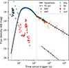 |
Fig. 1. Multi-wavelength light curve of GRB 250702F. Optical data from D50 are shown together with Swift/BAT and XRT observations. Multi-filter optical points have been colour-corrected to the r-band using the measured spectral slope. Open symbols represent General Coordinates Network (GCN) points. The solid line shows an empirical fit to the optical data (see Sect. 4). |
3. Prompt emission
To probe the origin of optical flare A (30–100 s), we performed time-resolved spectral analysis of the contemporaneous Fermi/GBM emission (Appendix B.1) in two intervals: SP1 (28.5–38.5 s) and SP2 (39.7–49.7 s). In both cases, the spectra are well fit by a cut-off power-law model. For SP1, we found a low-energy photon index of  and a peak energy of
  keV, while SP2 yielded αX = −1.49 ± 0.07 and Ep > 2 MeV.
Extrapolation of the best-fit models to optical frequencies predicts fluxes consistent with the observed D50 measurements (Fig. 2, bottom left panel). Combined with the temporal coincidence of flare A with the brightest MeV pulses, this supports a common origin in internal dissipation within the relativistic jet. The optical emission during this phase is not a separate afterglow component but rather the low-energy extension of the prompt spectrum.
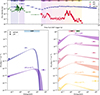 |
Fig. 2. Multi-wavelength light curves (top panel), spectral energy distributions, and modelling during the prompt phase (bottom-left panel) and during the X-ray flares (bottom-right panel). The optical data points from D50 and the LAT upper limits are shown together with the best-fit spectral models. During the prompt phase (SP1, SP2), the extrapolated gamma-ray spectrum is consistent with the observed optical flux. During the X-ray flares (SP3–SP8), the optical flux was set as an upper limit for the joint fit. |
After t ∼ 100 s, the GRB continues flaring in X-rays (Appendix B.2), with flux enhancements of roughly 10–100 times above any underlying power-law decay. By this point, the optical emission has decoupled and shows no corresponding re-brightenings. Joint XRT–BAT spectral analysis for six time intervals (SP3–SP8), with priors stipulating that the extrapolated spectrum does not exceed the observed optical flux, yielded smoothly broken power-law fits with peak energies from ∼0.1 keV to ∼4 keV and photon indices of αX ≈ −0.8 and βX ≈ −2.2 to −2.4 (Fig. 2, bottom-right panel). These spectral shapes match typical photon indices of MeV prompt emission pulses (Nava et al. 2012), supporting X-ray flares being softer analogues of prompt emission pulses. Fermi/LAT upper limits (0.1–1 GeV) lie above the extrapolated spectra and do not constrain the spectral shape further.
4. Optical light curve analysis
4.1. Empirical characterisation
Beyond t ∼ 100 s, the optical light curve shows a rapid rise transitioning to a flat maximum around t ∼ 200 s. This is followed by gradual steepening into a decay phase reaching α ∼ 1.6–2.0 (steepest just before t ∼ 1400 s), then a sharp break to a shallower power-law decline, α ∼ 0.8, that persists to late times.
We fitted the light curve with an empirical model consisting of a double hyperbola (capturing rise, plateau, and steep decay) joined to a late-time power law constrained by forward-shock closure relations (Appendix C). The best-fit parameters are the following: rise index 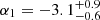 , plateau index
  , and steep decay index
  , with transition times at
  s and
s and  s. The break to standard afterglow behaviour occurs at
  s. The late-time decay is well described by an electron distribution index of p = 2.05 ± 0.04, yielding α4 = 0.79 ± 0.03 and a spectral slope of β = 0.52 ± 0.02 via interstellar medium slow-cooling closure relations.
The steep-to-normal decline (> 800 s) is incompatible with the standard forward-shock scenario (Sari et al. 1998). The rapid rise and steep decay are broadly consistent with emission from electrons in the GRB ejecta heated by a reverse shock (e.g. Nakar & Piran 2004). However, the presence of a shallow segment is difficult to reconcile with the standard picture of a single, homogeneous shocked shell. Moreover, in the reverse plus external forward-shock scenario, the deceleration time of both components are expected to coincide, which is inconsistent with the data (see Appendices D and F).
4.2. Thermal electron interpretation
We considered a forward-shock model with a hybrid electron distribution: a thermal (Maxwellian) component smoothly connected to a non-thermal power-law tail (Giannios & Spitkovsky 2009). The thermal population produces a synchrotron peak at frequency νth initially above the optical band. As the shock decelerates, νth ∝ t−3/2 sweeps through the optical band, producing the observed plateau followed by steep decay. Once the thermal contribution fades, the standard non-thermal afterglow emerges at t ∼ 1400 s.
Fitting this model to the optical data at t > 100 s (top panel of Fig. 3; Appendix E) yielded a non-thermal fraction of δ = 0.84 ± 0.02, an electron index p = 2.05 ± 0.01, deceleration time tdec = 175 ± 1 s, and a synchrotron frequency of thermal electrons at the time of deceleration of log10(νth0/Hz) = 14.43 ± 0.01. Provided these constraints, we inferred the initial bulk Lorentz factor of the jet: Γ0 ≃ 160. Thus, the characteristic thermal Lorentz factor of electrons is γth ≈ 900, assuming an equipartition parameter for non-thermal electrons of ϵe = 0.05 (see Appendix E). The co-moving magnetic field strength at deceleration is B′∼1.4 G, corresponding to the magnetic equipartition parameter of ϵB ≈ 5 × 10⁻⁴, which is consistent with constraints from TeV afterglow modelling of several GRBs (see Miceli & Nava 2022 for the review). Given the inferred ϵB, we constrained the cooling synchrotron frequency at the time of deceleration to νc0 ≃ 4 × 10¹⁷ Hz. This allowed us to predict the X-ray afterglow, which is consistent with the XRT data (bottom panel of Fig. 3).
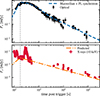 |
Fig. 3. Optical afterglow fit with a hybrid Maxwellian–power-law electron distribution model (top) and the corresponding X-ray prediction based on the optical fit (bottom). The steep decay emerges as the synchrotron frequency of thermal electrons sweeps through the optical band. |
5. Discussion
5.1. From prompt emission to X-ray flares
The spectral consistency between the observed optical emission and the extrapolated 8 keV–40 MeV spectrum during flare A implies a power-law extending across five decades in energy. During the brightest interval, SP1 (28.5–38.5 s), the low-energy photon index is αX ∼ −1.1. Within optically thin synchrotron self-Compton models, such a hard spectrum requires dominant inverse-Compton cooling in the Klein–Nishina regime (Derishev et al. 2001; Daigne et al. 2011), implying low magnetic fields (B′∼1–10 G) and electron energies of the TeV scale (Beniamini & Piran 2013; Ravasio et al. 2019). In the subsequent interval, SP2 (39.7–49.7 s), the spectrum softens to αX ∼ −1.5, consistent with fast-cooling electrons and indicating rapid evolution of the emission conditions. Such shallow low-energy slopes remain rare in time-resolved GRB spectra (e.g. Kaneko et al. 2006).
The X-ray flares detected during 100–500 s show spectral shapes similar to MeV prompt emission, namely smoothly broken power laws with αX ≈ −0.8 and βX ≈ −2.2 to −2.4, but with peak energies shifted to 0.1–4 keV (Sect. 3). This supports a physical link between prompt pulses and early X-ray flares as manifestations of continued internal dissipation (Chincarini et al. 2010; Margutti et al. 2010; Bernardini et al. 2011), which are distinct from the external-shock-driven optical afterglow.
5.2. Physics of thermal electrons
A key aspect of our interpretation requires clarification. The characteristic Lorentz factor of the thermal electrons, γth ≈ 900, is a few times larger than the bulk Lorentz factor of the shock, Γ0 ≈ 160. This may seem counterintuitive, as one might naively expect thermal electrons to simply have the bulk kinetic energy converted to random motion, yielding γth ∼ Γ0.
However, particle-in-cell (PIC) simulations of ultra-relativistic collisionless shocks (Spitkovsky 2008; Sironi et al. 2013) demonstrate that energy is approximately equipartitioned between protons and electrons in the downstream region. Electrons are energised far beyond the simple conversion of bulk to thermal energy. The characteristic thermal Lorentz factor for δ ≈ 0.8 scales as
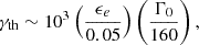 (1)
(1)
where ϵe is the fraction of shock energy deposited into electrons. This energisation is a fundamental prediction of collisionless shock physics and has been confirmed in numerous PIC studies (Sironi & Spitkovsky 2011; Warren et al. 2017).
The inferred fraction of energy in non-thermal electrons δ ≈ 0.8 implies that the shock acceleration operates, converting most of the electron energy into a power-law tail, while approximately 20% remains in the thermal pool. This is consistent with PIC simulation results showing that acceleration is efficient but not complete (Sironi et al. 2013; Warren et al. 2017, 2022).
6. Conclusions
We have presented multi-wavelength observations of GRB 250702F, for which the Ondřejov D50 robotic telescope obtained high-cadence optical coverage starting just 27.8 s after trigger – contemporaneous with the brightest MeV prompt emission pulses.
The early optical flare (30–100 s) is spectrally consistent with the MeV prompt emission, with the extrapolated gamma-ray spectrum correctly predicting the optical flux. This confirms a common origin in internal jet dissipation and provides rare spectral coverage spanning five decades in energy.
The subsequent optical evolution (100–1400 s) exhibits an unusual rise–stationary–steep-decay morphology that transitions sharply to a standard power-law afterglow at t ∼ 1400 s. Standard forward-shock and reverse-shock models fail to explain this morphology (Sect. 4).
The steep decay is naturally explained by a hybrid electron distribution at the forward shock, consisting of a thermal (Maxwellian) component smoothly connected to a non-thermal power-law tail. As the shock decelerates, the synchrotron peak of the thermal electrons sweeps through the optical band, producing the observed steep decay. The standard non-thermal afterglow then emerges.
The model fitting we performed yielded a non-thermal energy fraction of δ = 0.84 ± 0.02, an electron index of p = 2.05 ± 0.01, and a characteristic thermal Lorentz factor of γth ≈ 900. The inferred ϵB ≈ 5 × 10⁻⁴ is consistent with recent TeV afterglow constraints. These observations provide evidence for thermal electron signatures predicted by PIC simulations, enabled by the combination of early coverage, high cadence, and negligible host extinction.
Acknowledgments
We thank Emanuele Sobacchi and Pasquale Blasi for the fruitful discussions. BB acknowledges financial support from the Italian Ministry of University and Research (MUR) for the PRIN grant METE under contract no. 2020KB33TP. This research has made use of data obtained through the High Energy Astrophysics Science Archive Research Center Online Service, provided by the NASA/Goddard Space Flight Center, and specifically this work made use of public Fermi-GBM and Fermi-LAT data. This work made use of data supplied by the UK Swift Science Data Centre at the University of Leicester. The critical early-time observations were obtained with the 0.5-m robotic telescope D50 at the Astronomical Institute of the Czech Academy of Sciences in Ondrejov, supported by the project RVO:67985815.
References
- Akerlof, C., Balsano, R., Barthelmy, S., et al. 1999, Nature, 398, 400 [NASA ADS] [CrossRef] [Google Scholar]
- An, J., Noysena, K., Chanchaiworawit, K., et al. 2025, GCN Circular 40916 [Google Scholar]
- Angulo, C., Pereyra, M., Alan Watson, M., et al. 2025, GCN Circular 40907 [Google Scholar]
- Antier, S., Karpov, S., de Bruin, E., et al. 2025, GCN Circular 41011 [Google Scholar]
- Beniamini, P., & Piran, T. 2013, ApJ, 769, 69 [Google Scholar]
- Bernardini, M. G., Margutti, R., Chincarini, G., Guidorzi, C., & Mao, J. 2011, A&A, 526, A27 [NASA ADS] [CrossRef] [EDP Sciences] [Google Scholar]
- Beskin, G., Karpov, S., Bondar, S., et al. 2010, ApJ, 719, L10 [NASA ADS] [CrossRef] [Google Scholar]
- Brivio, R., Ferro, M., D’Avanzo, P., & Covino, S. 2025, GCN Circular 40913 [Google Scholar]
- Chincarini, G., Mao, J., Margutti, R., et al. 2010, MNRAS, 406, 2113 [NASA ADS] [CrossRef] [Google Scholar]
- Daigne, F., Bošnjak, Ž., & Dubus, G. 2011, A&A, 526, A110 [NASA ADS] [CrossRef] [EDP Sciences] [Google Scholar]
- de Ugarte Postigo, A., Thöne, C. C., Bolmer, J., et al. 2018, A&A, 620, A119 [NASA ADS] [CrossRef] [EDP Sciences] [Google Scholar]
- de Ugarte Postigo, A., Martin-Carrillo, A., Malesani, D. B., et al. 2025, GCN Circular 40901 [Google Scholar]
- Derishev, E. V., Kocharovsky, V. V., & Kocharovsky, V. V. 2001, A&A, 372, 1071 [NASA ADS] [CrossRef] [EDP Sciences] [Google Scholar]
- Evans, P. A., Beardmore, A. P., Page, K. L., et al. 2009, MNRAS, 397, 1177 [Google Scholar]
- Evans, P. A., Willingale, R., Osborne, J. P., et al. 2010, A&A, 519, A102 [NASA ADS] [CrossRef] [EDP Sciences] [Google Scholar]
- Fermi GBM team. 2025, GCN Circular 40892 [Google Scholar]
- Foreman-Mackey, D., Hogg, D. W., Lang, D., & Goodman, J. 2013, PASP, 125, 306 [Google Scholar]
- Fox, D. W., Yost, S., Kulkarni, S. R., et al. 2003, Nature, 422, 284 [Google Scholar]
- Frederiks, D., Ridnaia, A., Svinkin, D., et al. 2025, GCN Circular 40948 [Google Scholar]
- Giannios, D., & Spitkovsky, A. 2009, MNRAS, 400, 330 [NASA ADS] [CrossRef] [Google Scholar]
- Gomboc, A., Kobayashi, S., Guidorzi, C., et al. 2008, ApJ, 687, 443 [NASA ADS] [CrossRef] [Google Scholar]
- Jelínek, M. 2023, CAOSP, 53, 127 [Google Scholar]
- Kaneko, Y., Preece, R. D., Briggs, M. S., et al. 2006, ApJS, 166, 298 [CrossRef] [Google Scholar]
- Klingler, N. J., D’Ai, A., Gupta, R., et al. 2025, GCN Circular 40894 [Google Scholar]
- Komesh, T., Grossan, B., Maksut, Z., et al. 2023, MNRAS, 520, 6104 [Google Scholar]
- Kumar, A., O’Neill, D., Gompertz, B. P., et al. 2025, GCN Circular 40896 [Google Scholar]
- Lipunov, V., Gorbovskoy, E., Kuznetsov, A., et al. 2025, GCN Circular 40899 [Google Scholar]
- Margutti, R., Guidorzi, C., Chincarini, G., et al. 2010, MNRAS, 406, 2149 [NASA ADS] [CrossRef] [Google Scholar]
- Martin-Carrillo, A., Malesani, D. B., Radboud, et al. 2025, GCN Circular 40900 [Google Scholar]
- Mészáros, P., & Rees, M. J. 1997, ApJ, 476, 232 [CrossRef] [Google Scholar]
- Miceli, D., & Nava, L. 2022, Galaxies, 10, 66 [NASA ADS] [CrossRef] [Google Scholar]
- Nakar, E., & Piran, T. 2004, MNRAS, 353, 647 [CrossRef] [Google Scholar]
- Nava, L., Salvaterra, R., Ghirlanda, G., et al. 2012, MNRAS, 421, 1256 [Google Scholar]
- Racusin, J. L., Karpov, S. V., Sokolowski, M., et al. 2008, Nature, 455, 183 [Google Scholar]
- Ravasio, M. E., Ghirlanda, G., Nava, L., & Ghisellini, G. 2019, A&A, 625, A60 [NASA ADS] [CrossRef] [EDP Sciences] [Google Scholar]
- Sari, R., Piran, T., & Narayan, R. 1998, ApJ, 497, L17 [Google Scholar]
- Sironi, L., & Spitkovsky, A. 2011, ApJ, 726, 75 [NASA ADS] [CrossRef] [Google Scholar]
- Sironi, L., Spitkovsky, A., & Arons, J. 2013, ApJ, 771, 54 [Google Scholar]
- Spitkovsky, A. 2008, ApJ, 682, L5 [NASA ADS] [CrossRef] [Google Scholar]
- Štrobl, J., Jelínek, M., Polášek, C., & Hudec, R. 2023, CAOSP, 53, 49 [Google Scholar]
- Tonry, J. L., Denneau, L., Flewelling, H., et al. 2018, ApJ, 867, 105 [NASA ADS] [CrossRef] [Google Scholar]
- Vestrand, W. T., Wozniak, P. R., Wren, J. A., et al. 2005, Nature, 435, 178 [NASA ADS] [CrossRef] [Google Scholar]
- Vestrand, W. T., Wren, J. A., Wozniak, P. R., et al. 2006, Nature, 442, 172 [Google Scholar]
- Warren, D. C., Ellison, D. C., Barkov, M. V., & Nagataki, S. 2017, ApJ, 835, 248 [Google Scholar]
- Warren, D. C., Dainotti, M., Barkov, M. V., et al. 2022, ApJ, 924, 40 [NASA ADS] [CrossRef] [Google Scholar]
Appendix A: Optical observations
The Ondřejov D50 robotic telescope (Štrobl et al. 2023), operating under autonomous control via the RTS2 system, began unfiltered observations 27.8 s after the Swift trigger. Data were processed in real-time through the automated photometric pipeline (Jelínek 2023). Observations switched to photometric filters (g, r, i) approximately 15 minutes after trigger. Our best optical position for the afterglow, derived from D50 astrometry using Gaia DR3 reference stars corrected for proper motion and parallax, is R.A.  , Dec.
  (J2000), with uncertainties of
  in each coordinate.
The optical photometry presented in Table F.1 was obtained with the Ondřejov D50 telescope and reduced using the pyrt photometric pipeline (Jelínek 2023). This software performs ensemble photometry by fitting precise photometric zeropoints using large numbers of field stars from the Atlas-Refcat2 catalogue (Tonry et al. 2018), simultaneously solving for synthetic flat-field corrections and multi-filter colour terms.
Unfiltered (N) observations were calibrated against Atlas-Refcat2, yielding AB magnitudes equivalent to the r-band. For the afterglow spectral slope β = 0.52 (corresponding to g − r ≈ 0.17 mag and r − i ≈ 0.13 mag including Galactic extinction), the theoretical colour correction between unfiltered and r-band is ≲0.01 mag. This is consistent with the fitted zeropoint offset of 0.08 ± 0.05 mag (Appendix C), confirming that unfiltered photometry can be treated as r-band equivalent. Filtered observations (g, r, i) were calibrated using the respective filter passbands. The late-time GTC upper limit was obtained from a 400 s r-band exposure at ∼57 days post-burst.
Extensive optical follow-up was also performed by other facilities; their measurements reported in GCN Circulars (e.g. Kumar et al. 2025; Lipunov et al. 2025; Martin-Carrillo et al. 2025; Angulo et al. 2025; Brivio et al. 2025; An et al. 2025; Antier et al. 2025) are shown in Fig. 1 for comparison but not included in the model fitting due to uncertain cross-instrument zeropoints.
Appendix B: High-energy observations and data analysis
The burst GRB 250702F was detected by Fermi/GBM and independently triggered by Swift/BAT on 2025 July 2 at 21:06:43 UT (Fermi GBM team 2025; Klingler et al. 2025). The prompt emission showed a complex temporal structure extending from ∼3 s before to ∼80 s after the BAT trigger, with T90 (15–350 keV) of 63.7 ± 12.5 s.
Swift initiated rapid follow-up with XRT and UVOT, with the first XRT observation at 88.5 s post-trigger. Spectroscopy with the 10.4m GTC/OSIRIS+ measured a redshift of z = 1.520 (de Ugarte Postigo et al. 2025). The isotropic-equivalent energy Eiso = (9.9 ± 1.5)×1052 erg was derived from Konus-Wind data (Frederiks et al. 2025).
B.1. Fermi GBM
We retrieved the Fermi/GBM data (8 keV–40 MeV) of GRB 250702F from the Fermi GBM Burst Catalog and performed standard data reduction using the Fermi Science Tool GTBURST. We analysed data from the two sodium iodide (NaI; 8–900 keV) detectors and one bismuth germanate (BGO; 0.3–40 MeV) detector with the most favourable observing conditions, namely NaI-3, NaI-6, and BGO-0. The background was modelled by selecting custom time intervals free of source emission, spanning −110 s to −20 s before the trigger and 70 s to 150 s after the trigger, which allowed for a stable polynomial background fit.
We fitted the GBM time-resolved spectra during the prompt emission phase (SP1–SP2) in the 10–40000 keV energy range using a cutoff power-law model. The best-fit parameters are reported in Table B.1. The spectral peak energy, Ep, and the cutoff energy, Ecut, are related through Ep = (2 + αX)Ecut. The resulting spectral models are shown in Fig. 2, where they are extrapolated to the optical energy range for comparison with the D50 observations.
Spectral parameters for cutoff power-law model fits to prompt emission spectra.
B.2. Swift XRT and BAT
We retrieved the XRT and BAT light curves from the burst analyser web tool provided by the Swift Science Data Center (Evans et al. 2010). XRT spectral files in both WT and PC modes, along with corresponding background files, redistribution matrices, and ancillary response files, were obtained using the automated online spectral analysis tool (Evans et al. 2009).
Swift/BAT spectra were extracted using the HEASOFT software package (v6.33.1). The BAT event files were retrieved from the Swift data archive and processed with the batgrbproduct pipeline. Spectral files were generated using batbinevt and corrected for systematic uncertainties with batupdatephakw and batphasyserr. Response matrices were produced using batdrmgen.
We performed time-resolved joint XRT and BAT spectral fits for each time bin (SP3–SP8) in the 0.3–150 keV band using a smoothly broken power-law (sBPL) model. Since the optical emission shows no rebrightening during the X-ray flares, we required the extrapolated spectrum to lie below the observed optical flux by imposing a prior on the flux in the 1.8–3.1 eV range. The results are presented in Table B.2.
Spectral parameters for sBPL model fits to X-ray flare spectra.
B.3. Fermi LAT
We performed unbinned likelihood analysis of Fermi/LAT data for GRB 250702F (t0 = 773183208.102 s MET) extending to t0 + 1 ks, in the energy range 0.1–10 GeV, using the GTBURST software. We selected a region of interest covering 12° around the source location (R.A. = 212.93°, Dec. = 16.69°, J2000). A standard zenith angle cut of 100° was applied to remove Earth-limb contamination. We used the P8R3_TRANSIENT020 event class with corresponding instrument response functions, and included the isotropic particle background and 4FGL catalogue sources with fixed normalisation.
The source is not significantly detected in any time bin (TS < 25). A marginal excess (TS ∼18) is observed in SP8, with the highest-energy photon (∼4.5 GeV) having association probability > 0.9. The 95% confidence upper limits are reported in Table B.3.
LAT time-resolved analysis results.
Appendix C: Empirical optical light curve modelling
We fitted the optical light curve at t > 100 s (Fig. 1) with a model consisting of two components joined at a sharp break time tb. For t < tb, we use a double hyperbola that smoothly transitions through three power-law segments with asymptotic slopes α1 (rise), α2 (plateau), and α3 (steep decay), with vertex times tv, 1 and tv, 2 controlling the transitions. For t > tb, the light curve follows a standard forward-shock power-law decay constrained by closure relations: the temporal slope α4 = 3(p − 1)/4 and spectral slope β = (p − 1)/2 are both determined by the electron index p, appropriate for ν < νc in a homogeneous medium.
We adopted uniform priors on the model parameters (see Table C.1) and sampled the posterior distribution using Markov Chain Monte Carlo (MCMC) with the emcee package (Foreman-Mackey et al. 2013), fitting 80 D50 photometric points. A zeropoint offset between unfiltered and r-band observations was included as a nuisance parameter; the fitted value (0.08 ± 0.05 mag) is consistent with zero. The fit achieves χ2/dof = 82/68 = 1.2.
Model parameters and prior distributions for the empirical light curve fit.
Appendix D: Two-component fit of the optical light curve
To test the reverse-shock interpretation, we fitted the optical light curve (>100 s) with a two-component model: a smoothly broken power law (SBPL), describing the underlying forward-shock (FS), and a superposed double smoothly broken power law (2SBPL), representing the reverse-shock (RS). Both components were modelled with independent break times, normalisations and temporal indices, as shown in Fig. D.1. We adopted uniform priors on the model parameters (see Table D.1), and sampled the posterior distribution using the MCMC method implemented with the emcee package (Foreman-Mackey et al. 2013). The fit results are reported in Table D.1.
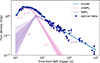 |
Fig. D.1. Two-component (RS + FS) fit to the optical light curve. The inferred RS peak time does not coincide with the FS peak, contrary to the expectation that both components originate from the same deceleration radius. |
Model parameters and prior distributions for the two-component optical light curve fit.
The key prediction of RS models is that the RS and FS should peak at approximately the same time, since both arise from the deceleration of the ejecta at the same radius. In our fits, however, the inferred RS peak time (tpeak, RS ∼ 400–600 s) is significantly later than the FS peak (tpeak, FS ∼ 100–200 s, corresponding to the deceleration time). This temporal offset cannot be reconciled with standard RS theory.
Furthermore, the extended stationary phase (α ≈ 0 between 200–600 s) requires fine-tuning in the two-component model: the RS decay and FS rise must nearly cancel over an extended period, which is not a natural outcome of the physics. In contrast, the thermal electron model (Appendix E) produces the stationary phase naturally as the thermal synchrotron peak frequency passes through the optical band.
Appendix E: Hybrid electron distribution model
To model the optical light curve at t ≳ 100 s, we adopt a hybrid electron energy distribution consisting of a thermal (Maxwellian) component and a non-thermal power-law tail, following Giannios & Spitkovsky (2009, hereafter GS09). Electrons crossing the relativistic forward shock populate a relativistic Maxwellian at low energies, with a fraction subsequently accelerated into a power-law tail. The electron distribution is
 (E.1)
(E.1)
where
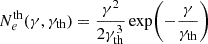 (E.2)
(E.2)
is the relativistic Maxwellian distribution. Here γth is the characteristic thermal Lorentz factor, γm is the minimum Lorentz factor of the power-law tail, p is the power-law index, and C is a normalisation constant.
The distribution is parameterised by: (i) the fraction δ of electron energy in the non-thermal tail, (ii) the characteristic thermal Lorentz factor γth, and (iii) characteristic Lorentz factor of electrons γc above which electrons lose their energy on a dynamical time-scale. We assume slow cooling regime (γc > γm) throughout, where γm is the minimum Lorentz factor of non-thermal electrons.
Our phenomenological model parameters are: (1) δ, (2) the thermal synchrotron frequency at deceleration νth0, (3) the cooling frequency νc0, at the deceleration time (4) the power-law index p of non-thermal electrons, and (5) the deceleration time tdec. For t < tdec, we assume Fν ∝ t3 (coasting phase). At later times, νth(t) = νth0(t/tdec)−3/2.
Best-fit parameters are: δ = 0.84 ± 0.02, p = 2.05 ± 0.01, tdec = 175 ± 1 s, and log10(νth0/Hz) = 14.43 ± 0.01. The initial bulk Lorentz factor is (homogeneous medium)
 (E.3)
(E.3)
Assuming ϵe = 0.05 and Γ0 ≃ 160, we infer γth ≃ 900.
The co-moving magnetic field strength is B′≃1.4 G, corresponding to
 (E.4)
(E.4)
The cooling frequency at deceleration is νc0 ≃ 4 × 10¹⁷ Hz, evolving as νc(t) = νc0(t/tdec)−1/2 (homogeneous medium).
Appendix F: Archival GRB comparison
We searched for similar rise–stationary–steep-decay structures in archival GRB optical light curves. GRB 161023A (de Ugarte Postigo et al. 2018) exhibits morphologically similar behaviour. However, the temporal slope (3p − 1)/4 with p ≈ 2.5 recurs at multiple stages of the afterglow decay, the post-jet-break decline is consistent with the same p, and the spectral slope β ≈ (p − 1)/2 with moderate extinction is maintained throughout. This makes GRB 161023A a conclusive high-p case, with the steep-to-shallow transition naturally attributed to energy injection.
Burst GRB 050820A (Vestrand et al. 2006) also shows prompt optical pulses followed by a rapid rise transitioning into an afterglow decay, with a steep decay section that has not been fully accounted for by previous modelling. Fitting the optical light curve with the hybrid electron model yields an acceptable solution (δ ≈ 0.2, p ≈ 2.6, χ2/dof ≈ 1.5). However, the steeper observed spectral energy distribution is equally consistent with a standard high-p forward shock with moderate host extinction and energy injection episodes, so the thermal electron interpretation provides no advantage over the traditional scenario.
A more compelling case appears in GRB 201015A (FRAM, unpublished), where a similar structure is observed at lower signal-to-noise and available multi-colour data (Komesh et al. 2023) seem to favour a thermal electron interpretation. This suggests that the light curve morphology discussed here may not be unique to GRB 250702F, and that further cases may be identified with sufficiently early and well-sampled multi-colour coverage.
The key distinction of GRB 250702F is its negligible host extinction (AV ≈ 0), which directly constrains the intrinsic spectral slope and firmly locks p = 2.05. This removes the β–extinction degeneracy that can otherwise mask the true electron index. The combination of well-sampled early optical coverage and clean spectral energy distribution constraints makes GRB 250702F uniquely suited for testing the thermal electron scenario.
Photometric observations of GRB 250702F.
All Tables
Spectral parameters for cutoff power-law model fits to prompt emission spectra.
Model parameters and prior distributions for the two-component optical light curve fit.
All Figures
|
Fig. 1. Multi-wavelength light curve of GRB 250702F. Optical data from D50 are shown together with Swift/BAT and XRT observations. Multi-filter optical points have been colour-corrected to the r-band using the measured spectral slope. Open symbols represent General Coordinates Network (GCN) points. The solid line shows an empirical fit to the optical data (see Sect. 4). |
| In the text | |
|
Fig. 2. Multi-wavelength light curves (top panel), spectral energy distributions, and modelling during the prompt phase (bottom-left panel) and during the X-ray flares (bottom-right panel). The optical data points from D50 and the LAT upper limits are shown together with the best-fit spectral models. During the prompt phase (SP1, SP2), the extrapolated gamma-ray spectrum is consistent with the observed optical flux. During the X-ray flares (SP3–SP8), the optical flux was set as an upper limit for the joint fit. |
| In the text | |
|
Fig. 3. Optical afterglow fit with a hybrid Maxwellian–power-law electron distribution model (top) and the corresponding X-ray prediction based on the optical fit (bottom). The steep decay emerges as the synchrotron frequency of thermal electrons sweeps through the optical band. |
| In the text | |
|
Fig. D.1. Two-component (RS + FS) fit to the optical light curve. The inferred RS peak time does not coincide with the FS peak, contrary to the expectation that both components originate from the same deceleration radius. |
| In the text | |
Current usage metrics show cumulative count of Article Views (full-text article views including HTML views, PDF and ePub downloads, according to the available data) and Abstracts Views on Vision4Press platform.
Data correspond to usage on the plateform after 2015. The current usage metrics is available 48-96 hours after online publication and is updated daily on week days.
Initial download of the metrics may take a while.