


| Issue |
A&A
Volume 710, June 2026
|
|
|---|---|---|
| Article Number | A47 | |
| Number of page(s) | 16 | |
| Section | Astrophysical processes | |
| DOI | https://doi.org/10.1051/0004-6361/202659489 | |
| Published online | 29 May 2026 | |
The singular behaviour of ambipolar diffusion revealed by 1D Cartesian solutions
1
Instituto de Astrofísica de Canarias, 38205 La Laguna, Tenerife, Spain
2
Departamento de Astrofísica, Universidad de La Laguna, 38206 La Laguna, Tenerife, Spain
3
School of Mathematics and Statistics, University of St Andrews, St Andrews, KY16 9SS, UK
4
Rosseland Centre for Solar Physics, University of Oslo, PO Box 1029 Blindern N-0315, Oslo, Norway
5
Institute of Theoretical Astrophysics, University of Oslo, PO Box 1029 Blindern N-0315, Oslo, Norway
★ Corresponding author: This email address is being protected from spambots. You need JavaScript enabled to view it.
Received:
17
February
2026
Accepted:
1
April
2026
Abstract
Context. Ambipolar diffusion is increasingly recognised as a key process in the lower solar atmosphere. Its highly non-linear behaviour has many non-intuitive aspects.
Aims. We seek to (a) study 1D Cartesian ambipolar diffusion near null points; (b) characterise the non-linear eigenmodes for ambipolar diffusion; and (c) propose tests for ambipolar diffusion solvers in MHD codes.
Methods. (a) We employed a direct analysis to obtain analytical solutions for ambipolar diffusion. (b) To study the eigenmodes, we solved the ODE for self-similar solutions of the 1D ambipolar diffusion equation using phase-plane techniques. We also solved the general time-dependent 1D problem for initial conditions of interest. (c) We tested the Bifrost code by trying to reproduce the behaviour of the eigenmodes.
Results. (a) A stagnation-point flow solution was found with a uniform flux transfer rate across three regions: an external advection region; an internal ambipolar diffusion region with magnetic profile B ∝ x1/3; and an innermost Ohmic region with B ∝ x; in the latter, flux annihilation occurs at a rate imposed by the advection. (b) Both symmetric and antisymmetric eigenmode solutions to the ambipolar diffusion problem were found with sharp current sheets at the internal nulls. The time evolution of the eigenmodes (pure or perturbed) was probed, showing how higher order eigenmodes, or perturbed ones, evolve over time towards the lowest order allowable eigenmodes. (c) The Bifrost code reproduces the behaviour of the eigenmodes with excellent accuracy.
Conclusions. Stagnation-point configurations exist with ambipolar diffusion carrying magnetic flux in an inner layer and serving as an intermediary between the external advection and the flux dissipation and annihilation at an Ohmic-diffusion core around the null. Our tests are compatible with the hypothesis that zero-flux higher harmonics of the self-similar equation evolve toward either the first symmetric or antisymmetric harmonic. The self-similar solutions can serve as strong tests for ambipolar diffusion solvers in general MHD codes.
Key words: diffusion / magnetic fields / plasmas / methods: analytical / methods: numerical
© The Authors 2026
 Open Access article, published by EDP Sciences, under the terms of the Creative Commons Attribution License (https://creativecommons.org/licenses/by/4.0), which permits unrestricted use, distribution, and reproduction in any medium, provided the original work is properly cited.
This article is published in open access under the Subscribe to Open model. This email address is being protected from spambots. You need JavaScript enabled to view it. to support open access publication.
1. Introduction
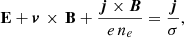
Ideal magnetohydrodynamics (MHD) is governed by the single-fluid, non-resistive form of Ohm’s law (E + v × B = 0) and has proven extremely useful to understand the physics of many simple situations when the plasma can be assumed to be fully ionised. Yet, for ideal (i.e. non-viscous and non-resistive) MHD, there is no way in which the magnetic energy, often the largest form of available energy, can be converted, directly or indirectly, into internal energy via dissipation. Remaining within the simplest single-fluid approximation for a fully ionised plasma, while including the drift between electrons and ions and their mutual friction, one obtains two additional terms in Ohm’s law, namely, the Hall term and the Ohmic diffusion term
 (1)
(1)
where σ = ne e2/(me νei), νei is the electron-ion collision frequency, and ne is the number density of electrons (Cowling 1957). In Eq. (1), the effect of the electron pressure has been neglected. The term on the right of the equation, the Ohmic term, is due to the electron-ion friction; it leads to an irreversible increase of the internal energy of the fluid at a rate j2/σ per unit time. We note that v (in the second term on the left and in most discussions of Ohm’s law in the literature) is the bulk velocity of the plasma (i.e., in this case, the ion velocity). The Hall term on the left results from the fact that, if the electron-ion friction were negligible, the magnetic field lines would be tied to the electron fluid (given the very small inertia of electrons).
Equation (1), often neglecting the Hall term, has been widely used in solving problems for fully ionised plasmas, such as those in the solar corona. However, in the lower part of the solar atmosphere, the photosphere and chromosphere, the plasma is not fully ionised. The neutral atoms can slip relative to the charged components; however, there is also a single-fluid approximation in which the friction between the neutral and charged species instantaneously adapts to the varying physical situations of the system, compensating for the difference in the forces acting on the charged and neutral particles (Cowling 1957; Braginskii 1965; Mitchner & Kruger 1973). This results in equations for mass conservation and momentum as in standard MHD for the global fluid (charged + neutrals), but Ohm’s law is changed due to the slippage of the magnetic field with respect to the neutrals.
Even if, for simplicity, we ignore the differential effect of the partial pressures of electrons, ions, and neutrals, the ions and neutrals will drift from each other with a drift speed vi − vn, which, following the assumption of instantaneous adjustment of the friction to the driving forces, can be given essentially by equalising the Lorentz force and the friction between the neutrals and the charged species, that is,
 (2)
(2)
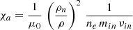
where min is the reduced ion-neutral mass, ρn the mass density of the neutrals, ρ the total mass density (ions+neutrals), ni the number density of the ions, νin the ion-neutral collision frequency, and μ0 the standard vacuum permeability; for simplicity, single-charged ions are assumed, so ni = ne. This slippage is called ambipolar diffusion; correspondingly, the generalised Ohm’s law just receives an extra term compared to Eq. (1) and becomes
 (3)
(3)
with
 (4)
(4)
and the symbol ⊥ indicating the component normal to the magnetic field. In Eq. (3), v stands for the centre-of-mass velocity of the plasma, as in Eq. (1), but now including both ions and neutrals. The factor ρn/ρ can be close to unity in situations where the degree of ionisation is low, as in the solar photosphere where the ionisation can be as low as 10−4. The plasma becomes completely ionised only above the upper chromosphere.
Taking the curl of Eq. (3) and using Faraday’s law turns it into a generalised induction equation which, for the simple case in which the Hall term can be neglected, can be written as
![Mathematical equation: $$ \begin{aligned} \frac{\partial \mathbf{B}}{\partial t}= {\boldsymbol{\nabla }}\times \left[\boldsymbol{v} \times \mathbf{B}\,-\, \eta \,{\boldsymbol{\nabla }}\times \boldsymbol{B} \, - \,\chi _a\,B^2\,({\boldsymbol{\nabla }}\times \boldsymbol{B})_\perp \right], \end{aligned} $$](/articles/aa/full_html/2026/06/aa59489-26/aa59489-26-eq5.gif) (5)
(5)
where η = 1/(σ μ0). The resulting internal energy equation in the presence of both Ohmic and ambipolar diffusion, but disregarding viscous dissipation, takes the form
 (6)
(6)
with ϵ the internal energy per unit mass and the symbol D/Dt indicating the material derivative (∂/∂t +v · ∇). Thus, both Ohmic and ambipolar diffusion can convert magnetic energy into heat as the magnetic field evolves, the former because of the electron-ion friction, the latter because of the friction between neutrals and charged species.
The magnitude of the ambipolar resistivity, χa B2, in the solar atmosphere remains a subject of debate; under the strong and often unrealistic assumption of LTE for the ionisation level of hydrogen, one would conclude that in the upper solar photosphere, ambipolar diffusion can be a factor of 10 greater than normal Ohmic diffusion. In the chromosphere, the factor rises to 103 in the quiet Sun or 105 in an active region (Khomenko & Collados 2012; Priest 2014); however, non-equilibrium ionisation effects can drastically change the importance of this effect (see Nóbrega-Siverio et al. 2020a; Wargnier et al. 2022; see also Hillier 2024).
Ambipolar diffusion differs in a number of important ways from normal Ohmic diffusion:
(i) it is a non-linear process in B, and so has many counter-intuitive effects;
(ii) it vanishes at null points unless the current becomes singular; in fact, it tends to steepen field profiles that contain a null into sharp current sheets (see also Sects. 2 and 6, where the possibilities of having annihilation and reconnection at the null via a small Ohmic region within an ambipolar-dominated domain are discussed).
(iii) the timescales are very different; for a length-scale L0 and magnetic field B0 the Ohmic diffusion timescale is
 (7)
(7)
whereas the ambipolar diffusion timescale is
 (8)
(8)
Thus, ambipolar diffusion is fastest in regions of high magnetic field. When ambipolar diffusion is stronger than Ohmic diffusion (as assumed in this paper), the former will be the dominant diffusion process in the induction equation, although Ohmic diffusion can still be relevant around null points.
In this paper we concentrate on a simple ‘plane-parallel’ situation in which  and the coefficients η and χa are uniform; we are also assuming a static plasma (except in Sect. 2.2), so that the induction equation (Eq. (5)) is reduced to
 (9)
(9)
which is a non-linear diffusion equation. We aim to determine explicit analytical solutions and numerical examples for this equation to highlight the mathematical and physical consequences of ambipolar diffusion in 1D Cartesian geometry and to explore their possible use in benchmarking ambipolar diffusion solvers in MHD codes.
This paper builds on work presented in a previous publication (Moreno-Insertis et al. 2022), where we studied solutions to the equivalent problem in a cylindrically symmetric situation and devised tests for MHD numerical codes that include an ambipolar diffusion solver. The ambipolar diffusion problem in either geometry admits signed self-similar solutions that are counterparts to the basic family of unsigned solutions for a large class of non-linear diffusion problems originally discovered by Zel’dovich & Kompaneets (1950), Barenblatt (1952), see also Pattle (1959), Zel’dovich & Raizer (1967), Vázquez (2007). The mathematical properties of all these solutions have been studied in depth in the applied mathematics literature (see e.g. Grundy 1979; Hulshof 1991; Vázquez 2007; and a brief summary in Moreno-Insertis et al. 2022).
The study of ambipolar diffusion in plasma physics started long ago (Cowling 1957) as did its applications to astrophysical plasmas (e.g. Parker 1963). Such applications are numerous and cover very different cosmic contexts. In the solar photosphere and chromosphere, the importance of ambipolar diffusion was stressed by Priest (1982) in his monograph on MHD; the interest on this phenomenon has gradually increased until the present. Solar physics applications include the excitation, propagation, and mode-conversion of MHD waves (e.g. Kumar & Roberts 2003; Vranjes et al. 2008; Soler et al. 2010; Zaqarashvili et al. 2011; Cally & Khomenko 2018), Kelvin-Helmholtz instability (Soler et al. 2012; Hillier 2019; Hillier et al. 2024), Rayleigh-Taylor instability (Ruderman et al. 2018), heating of the chromosphere (Goodman 2000, 2004; Khomenko & Collados 2012), magnetic reconnection (Parker 1963; Zweibel 1989; Heitsch & Zweibel 2003; Sakai & Smith 2009; Zweibel & Yamada 2009; Leake et al. 2012, 2013; Snow et al. 2018), and the tearing-mode instability (Ni et al. 2015, 2016, 2022; Cheng et al. 2024). Detailed computational modelling of its effects has been reported for the emergence of magnetic flux from below the solar photosphere (Leake & Arber 2006; Arber et al. 2007, 2009; Leake & Linton 2013; Nóbrega-Siverio et al. 2020b); for the fine structure of the solar photosphere and chromosphere (Martínez-Sykora et al. 2012, 2017a), particularly with respect to spicules (De Pontieu et al. 2017; Martínez-Sykora et al. 2017b, 2018, 2020); for the formation of structure in solar prominences (Khomenko et al. 2014, 2016); and for magnetoconvection (Khomenko et al. 2018).
In non-solar astrophysics, ambipolar diffusion is important in many similar physical processes, but under different parameter regimes, such as the structure of interstellar shock waves (Draine 1986; Draine & McKee 1993) and the formation of current sheets in the interstellar medium (Zweibel & Brandenburg 1997). It has also been considered as a mechanism for diffusion of magnetic flux in dense molecular clouds (Mestel & Spitzer 1956; Spitzer 1962), where it plays a key role in star formation (Shu 1983; Crutcher 1999; Mac Low & Klessen 2004; Nakamura & Li 2008; Ballester et al. 2018), magnetic braking (Mouschovias & Paleologou 1979; Li et al. 2014), and the formation of filamentary structure (Hennebelle & André 2013). Further numerical models in 2D and 3D that study the effects of ambipolar diffusion in molecular clouds are those of Kunz & Mouschovias (2010) and Tritsis (2025). In planetary ionospheres, ion-neutral coupling and therefore ambipolar diffusion is important in creating global currents and neutral winds (e.g. Bauer 1973; Pfaff 2012; Ballester et al. 2018).
In this paper, we start by giving an overview of past results concerning the B ∼ x1/3 profiles that naturally arise around null points in ambipolar diffusion contexts (Sect. 2.1). We then (Sect. 2.2) introduce a generalisation of the stagnation-point flow that includes both ambipolar and Ohmic diffusion terms. The second part of the paper is devoted to calculating self-similar solutions with compact support, both symmetric and antisymmetric, which have been shown in the literature to constitute a countable set (Sect. 3). Numerical solutions starting from various initial conditions permit an initial exploration of the stability of the self-similar solutions (Sect. 4). Section 5 illustrates the usefulness of the solutions in testing numerical codes with ambipolar diffusion solvers. Finally, Sects. 6 and 7 contain a discussion and conclusions, including multi-fluid considerations on the important differences between ohmic and ambipolar diffusion regarding magnetic flux conservation and annihilation.
2. General results from conservation theorems
Consider the induction equation for a static plasma with Ohmic and ambipolar terms, namely, Eq. (5) with v = 0. Integrating it over a surface S bounded by a curve C that does not change in time and using Stokes’ theorem gives
 (10)
(10)
with n the unit normal vector to the surface and τ the unit tangent vector to the curve. For the case of a 1D field,  , still with v = 0, the induction equation becomes Eq. (9), which can be rewritten as
 (11)
(11)
in terms of the total diffusive flux (i.e. the magnetic flux transfer rate in the diffusive regime), namely,
 (12)
(12)
which is the sum of the Ohmic and ambipolar diffusive fluxes. Next, Equation (11) may be integrated over x from a to b, say, to give the time-variation of the magnetic flux Φ as
![Mathematical equation: $$ \begin{aligned} \frac{d\Phi }{dt} = \frac{d}{dt}\int _a^b B\ dx= -[{F_{d}}]_a^b, \end{aligned} $$](/articles/aa/full_html/2026/06/aa59489-26/aa59489-26-eq15.gif) (13)
(13)
so that naturally the rate of change of magnetic flux is the difference between the total diffusive fluxes at the two boundaries.
From Eq. (11), the steady-state solution for the purely ambipolar problem requires Fd to be uniform; therefore, according to Eq. (12), dB3/dx must be uniform. When joining two values (e.g. B0 and B1) of the same sign at x = ±L0, the magnetic field is well behaved (as in the top curve of Fig. 1). When B0 and B1 have opposite signs, an x1/3 singularity appears where the solution crosses the x-axis (as in the two lower curves of Fig. 1). In the next subsection, we focus on the antisymmetric case (B1 = −B0, namely, the lowest curve in Fig. 1), while in Sect. 2.2, a stagnation flow solution is introduced, all within the single-fluid approach of the generalised Ohm’s law; a discussion of some multi-fluid considerations underlying the MHD solution and possibly limiting it is given in Sect. 6.
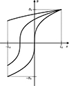 |
Fig. 1. Sketch of the solution for steady-state ambipolar diffusion joining B = B1 at x = −L0 to B = B0 at x = L0 for three different values of B1, namely, 2B0/3 (top curve), −2B0/3 (middle curve), and −B0 (bottom curve). |
2.1. Diffusive behaviour near null points, flux transfer, and annihilation
2.1.1. Parker’s 1963 solution
Null points play a special role in this problem: the ambipolar diffusive flux −χa B2 ∂B/∂x vanishes at them so that only the Ohmic diffusion term (or perhaps some collisionless diffusion process) can lead to magnetic flux annihilation. This was already recognised in a seminal paper by Parker (1963), who considered the problem of stationary solutions to the diffusion equation (Eqs. (11) and (12)). Assuming uniform coefficients χa and η, he obtained an exact solution of the general form
 (14)
(14)
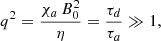
with c2 an arbitrary integration constant, in which the null is assumed to be located at x = 0. Clearly, that equation gives a behaviour of the kind B ∝ x1/3 wherever ambipolar diffusion dominates Ohmic diffusion, and a linear behaviour, B ∝ x, in the opposite case. Assume that the case at hand is ambipolar-diffusion-dominated almost everywhere; that is, more precisely, assume that for a generic point at a distance L0 from the origin (x = L0) with a field strength B0 the ratio of the first to the second term on the right hand side of (14) is high. Thus, we have
 (15)
(15)
with τd and τa as defined in Eqs. (7) and (8). In that case, (14) can be turned into
 (16)
(16)
This relation is depicted as the green curve in Fig. 2 (both in the main frame and in the inset). Parker (1963) noted that the solution
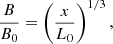 (17)
(17)
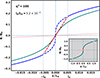 |
Fig. 2. Solution to the mixed Ohmic and ambipolar diffusion problem of Eqs. (11) and (12), in which the inset shows the whole range −L0 ≤ x ≤ L0) and the main frame shows just the central domain −0.018L0 ≤ x ≤ 0.018L0)]. Green: Exact solution (16). Blue: Purely ambipolar solution (17). Dashed red: Linear, purely Ohmic solution with slope at the origin equal to that of the full solution (19). Pink: Linear purely Ohmic solution linking the points ( − L0, −B0) and (L0, B0). The dotted vertical lines mark the locations x = ±ld. The blue and green curves and the red segment appear superimposed in the inset. |
illustrated by the blue curve in the main frame of the figure, is valid everywhere except in the immediate neighbourhood of the null point, which is Ohmic-diffusion-dominated: in the narrow range −ld ≤ x ≲ ld, with
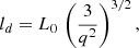 (18)
(18)
the solution is instead linear, namely,
 (19)
(19)
as shown by the dashed red straight line in the main frame of Fig. 2 (and the red segment in the inset). Parker’s conclusion was that ambipolar diffusion is not the dominant mechanism near the null, and that flux transfer and annihilation across the null are possible by Ohmic diffusion. Yet, due to the presence of ambipolar diffusion in most of the domain, the slope of the B-profile at the null, (B0/L0) q2/3 (the dashed red line in the figure), is much larger than given by a simple Ohmic diffusion solution in the whole domain (having slope B0/L0, the pink line in the main frame and in the inset). Correspondingly, Parker calculated that the total Joule dissipation in the small range −ld ≤ x ≤ ld for the Ohmic-dominated part of the whole solution is a factor q larger than that of the simple pure Ohmic solution in the range (0, L0).
2.1.2. The flux transfer rate in the B ∝ x1/3 profile
As an extension of the foregoing, we note the remarkable fact that in an ambipolar-diffusion-dominated region with profile B ∝ x1/3 (whether stationary or otherwise) the flux transfer rate (or diffusive flux) Fd is uniform: in that region the electric current has a steep profile jy ∼ x−2/3 approaching a singularity as x → 0, but the field goes to zero, so Fd = −(χa/μ0)jyB2= constant. Therefore, the ambipolar term will be passing flux to the Ohmic-dominated region at a uniform rate thanks to the steepness of the profiles in spite of the smallness of B. Flux dissipation and reconnection are then possible in the region around the null at rates determined by the ambipolar diffusion, even if not directly in the ambipolar-diffusion-dominated part of the domain.
In the stationary case, we can show that the flux transfer across the null in the combined Ohmic+ambipolar problem has the same intensity as for a purely ambipolar diffusion solution (17); to that end, we compare the Ohmic flux transfer rate η ∂B/∂x for the actual solution near the centre (19), namely, η B0 q2/(3 L0), with the transfer rate that would apply if the singular, purely ambipolar diffusion solution were valid there, namely, χa B2 ∂B/∂x with B given by Eq. (17): the two values are identical as can be easily checked by using the definition of q2. So, even when Ohmic diffusion prevails near the null, the flux transfer rate (and possible annihilation properties) is determined by ambipolar diffusion.
2.2. Stagnation-point flow
Parker (1973) considered a kinematic solution for the effect of a 2D stagnation-point flow on the induction equation alone including Ohmic diffusion, whereas Sonnerup & Priest (1975) extended this to a 3D stagnation-point flow and they showed that it represents one of the few exact solutions of MHD since it also satisfies the equation of motion. We can now extend the 2D solution to include ambipolar diffusion as follows.
Consider unidirectional oppositely directed magnetic fields,  , that are driven together by a stagnation-point flow of the form
 (20)
(20)
with v0 > 0, as indicated in the upper panel of Fig. 3. In a steady-state situation, Ohm’s law including advection, ambipolar diffusion and Ohmic diffusion may be written as
 (21)
(21)
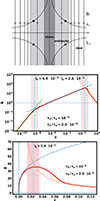 |
Fig. 3. Top: Schematic of a stagnation-point flow configuration, showing magnetic field lines (light-headed arrows) for a 1D current sheet together with a stagnation-point flow (solid-headed arrows). The ideal, ambipolar, and Ohmic regions are indicated. Middle and bottom: Solution of the dimensionless stagnation flow equation (Eq. (29)) with logarithmic (middle panel) and linear axes (bottom panel). Solid red: solution for |

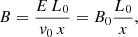
given the geometry and the condition ∇ × E = 0, the electric field must be uniform. Also, we want to seek antisymmetric solutions for B(x) and will thus discuss the solution for x > 0 only. To avoid infinities for large x, the effects of ambipolar and Ohmic diffusion must be negligible at large x. The solution in the asymptotic region (the ‘ideal’ region) is just given by
 (22)
(22)
where L0 is the coordinate of any point in that region and B0 the value of the field at it if exactly on the asymptotic curve. The natural timescale for the ideal region is the advective timescale defined by
 (23)
(23)
Suppose that the magnetic field vanishes at x = 0; as one goes inward from x = L0 toward x = 0, at some point the ambipolar and Ohmic diffusion effects will become relevant and eventually dominant. If, as in the foregoing section, the Ohmic diffusion overcomes the effects of ambipolar diffusion in a narrow region close to the centre only, then we will have three distinct regions in the problem, the outer one (the ideal solution), a middle one dominated by ambipolar diffusion and the central one, around x = 0, dominated by Ohmic diffusion. Assume the transition between the ideal and ambipolar-diffusion-dominated regions occurs around x = O(la), whereas the transition between ambipolar and Ohmic-diffusion-dominated regions is located at x = O(ld).
Clearly, wherever ambipolar diffusion dominates, the solution is given by
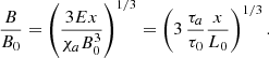 (24)
(24)
Thus, the extent (la) of the region dominated by ambipolar diffusion is given by the value of x that equates the ideal and ambipolar fields (22) and (24), namely,
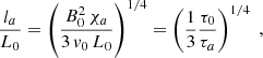 (25)
(25)
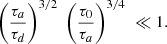
with τa as defined in Eq. (8), but now with the symbols L0 and B0 as used in the present section (see Eq. (22)). The condition that L0 is in the ideal region, i.e. la ≪ L0, is equivalent to the condition (τ0/τa)1/4 ≪ 1.
In the Ohmic diffusion region, on the other hand,
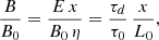 (26)
(26)
with τd as defined in Eq. (7), but now with the symbol L0 defined by Eq. (22); so the location (ld) where the transition between the ambipolar and Ohmic-dominated regions occurs is given by equating the fields in the ambipolar and Ohmic diffusion regions (24) and (26), namely,
 (27)
(27)
From Eqs. (25) and (27), whenever the condition la ≪ L0 is satisfied, then the condition ld ≪ la will also be satisfied in as far as the weaker additional requirement is fulfilled:
 (28)
(28)
One fact of particular interest is that, according to Ohm’s law (Eq. (21)), the flux transfer rate (i.e. the sum of the two diffusive terms and the advection term) is uniform in the whole domain. On the other hand, in each of the three regions just discussed only one of those terms is significant; therefore, it carries the whole magnetic flux in that region. Finally, in this problem, the magnetic flux inflow is determined by the external region (i.e. by advection). We see, therefore, that the advection inflow sets the value of the electric field and, with it, the overall flux transfer rate; the flux is then transferred by ambipolar and Ohmic diffusion in their respective domains at that same rate, which is also the flux annihilation rate in the innermost region.
To obtain the full magnetic field profile, we can use a dimensionless version of Eq. (21), namely:
 (29)
(29)
with  and
and  . We can then solve it using simple numerical means. The profile is shown in Fig. 3 (middle and bottom panels) for given choices of the parameters τ0/τd and τ0/τa. In this solution, the magnetic field is advected in by the flow from a distance x = L0 to around la, and then it diffuses inwards due to the diffusive flux (Eq. (12)). First of all, this field is carried by the ambipolar diffusive flux between about la and ld, and secondly by the Ohmic diffusive flux from about ld to the origin, where it is annihilated as it cancels with equal and opposite flux from x < 0.
3. General self-similar solutions
The analysis of self-similar solutions to the purely ambipolar diffusion equation, Eqs. (11) and (12) with η = 0, follows the same general scheme that we developed for symmetric solutions in a cylindrical geometry (Moreno-Insertis et al. 2022). However, here we are also dealing with antisymmetric solutions.
3.1. Basic solutions: the ZKBP and dipole solutions
The lowest order (i.e. fundamental) solutions to the ambipolar diffusion equation are particularly simple. The symmetric solution is
![Mathematical equation: $$ \begin{aligned} B(x,t) = \frac{B_{00}}{s_Z^(t)^{1/4}} \,\left\{ 1-\left[\frac{x}{L_{00}\, s_Z^(t)^{1/4}}\right]^2\right\} ^{1/2}, \end{aligned} $$](/articles/aa/full_html/2026/06/aa59489-26/aa59489-26-eq36.gif) (30)
(30)
where sz(t) = 1 + 4 t/t0 and t0 = L002/(χa B002). Here B00 and L00 represent the field strength at x = 0 and the spatial domain of the solution, respectively, both at t = 0. This is the basic solution for the general problem of non-linear diffusion in the particular case that the diffusion coefficient depends on the square of the variable being diffused; it is therefore the particular version for ambipolar diffusion of the fundamental Zeldovich-Kompaneets solution (Zel’dovich & Kompaneets 1950; Barenblatt 1952; Pattle 1959), also known in the mathematical literature as the Barenblatt solution. For simplicity, (30) is referred to as the ZKBP solution in the following. It is plotted, for x > 0, as the black curve in Fig. 4.
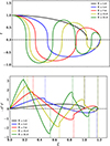 |
Fig. 4. Top: Fundamental (i.e. ZKBP) and first four symmetric harmonics as functions of the stretched coordinate |


In contrast, the lowest order antisymmetric solution is
![Mathematical equation: $$ \begin{aligned} B(x,t) = \frac{B_{00}}{s_d(t)^{1/3}}\; \left\{ 1- \left[\frac{x}{L_{00}\,s_d(t)^{1/6}}\right]^{4/3}\right\} ^{1/2} \; \left[\frac{ 6^{3/4}\,x}{L_{00}\,s_d(t)^{1/6}}\right]^{1/3} \,, \end{aligned} $$](/articles/aa/full_html/2026/06/aa59489-26/aa59489-26-eq39.gif) (31)
(31)
where  , while B00, L00, and t0 have the same meaning as above. This is known as the dipole solution and it was found by Zel’dovich & Barenblatt (1957, see also Zel’dovich & Raizer 1967); it is plotted, for x > 0, as the blue curve in Fig. 5. It possesses two lobes (for x < 0 and x > 0) that touch at the origin with an x1/3 profile. The ambipolar diffusive flux vanishes at the left and right end-points (
 ), but it does not vanish at the origin, so that, mathematically, flux can diffuse through the origin and cancel with flux from the opposite lobe. This is an example of the case discussed in Sect. 2.1 for pure ambipolar diffusion causing magnetic flux to cancel, with B vanishing but having an infinite gradient, although in fact the infinite gradient will be resolved by means of an inner Ohmic diffusion layer, as discussed in that section.
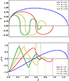 |
Fig. 5. Top: Fundamental (i.e. dipole) and first three antisymmetric harmonics as functions of the stretched coordinate |


3.2. The general self-similar formulation
The particular ambipolar solutions (30) and (31) are both of so-called self-similar form, namely, the variable x appears only in the combination x divided by a function of t, so here we seek more general self-similar ambipolar solutions in that form, namely,
 (32)
(32)
with f a function of the single variable ξ, while ℬ(t) and ℒ(t) are a time-dependent field strength and length scale, respectively, which are all to be determined as part of the solution. Then, the purely ambipolar diffusion equation can be reduced to
 (33)
(33)
where a dot and a prime denote ordinary derivatives with respect to t and ξ, respectively.
The resulting ambipolar diffusive flux (or rate of transport of magnetic flux) is given by Eq. (12) with η = 0 and so becomes
 (34)
(34)
We can normalise ℬ and ℒ with respect to values B00 and L00, respectively, at an initial time, t00, say, while the unit for time is set as t0 = L002/(χa B002). This is equivalent to setting χa = 1 in (33). Then the condition that the coefficients of f and ξf′ in Eq. (33) be constants K and H, respectively, gives
 (35)
(35)
The solutions of these equations are
![Mathematical equation: $$ \begin{aligned} {\mathcal{B}}(t) \; =\; \left[{\tau _{s}}(t)\right]^{\alpha },\quad \mathcal{L}(t) \; =\; \left[{\tau _{s}}(t)\right]^{\gamma }, \end{aligned} $$](/articles/aa/full_html/2026/06/aa59489-26/aa59489-26-eq48.gif) (36)
(36)
where
 (37)
(37)
and
 (38)
(38)
Our self-similar assumption has therefore reduced the partial differential ambipolar diffusion equation to an ordinary differential equation for f(ξ), namely,
 (39)
(39)
similar equations are found in the applied mathematics literature (Vázquez 2007; Hulshof 1991); it is our basic equation and it needs to be solved with boundary conditions that differ between the symmetric and antisymmetric cases.
3.3. The symmetric case
3.3.1. Boundary conditions
At the origin, we impose
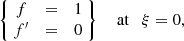 (40)
(40)
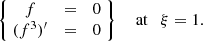
so, in this case, ℬ(t) is simply the magnetic field at the origin. Similarly to what was shown in detail in our previous paper (see Fig. 1 in Moreno-Insertis et al. 2022 and associated text), a continuum of solutions can be found for Eq. (39) which, in general, extend to infinity. Yet, we are interested in solutions with compact support; to obtain them, we also impose two conditions at an outer boundary, namely,
 (41)
(41)
The first of these is natural, but the second needs explanation. If B(x, t) did not change sign in the whole domain, it would be natural to impose constancy of magnetic flux, namely,
 (42)
(42)
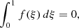
which leads to ℬ ℒ= const, K/H = 1, and therefore the ZKBP solution. However, we seek instead new self-similar solutions, namely, higher harmonics that possess zeros. In this case we impose instead
 (43)
(43)
which leads, after using Eqs. (39) and (40), to
 (44)
(44)
Physically, this corresponds to the vanishing of the diffusive flux at the outer expanding boundary so that the magnetic flux is confined in the domain.
3.3.2. Solutions
In order to find the eigenfunctions and eigenvalues for Eq. (39), we have adopted methods and techniques akin to those of Moreno-Insertis et al. (2022), using, in particular, a stretched variable  , defined as
  , and the coefficient
  , so that Eq. (39) is reduced to
 (45)
(45)
The boundary conditions (41) serve as quantisation rules, so that one finds a countably infinite series of solutions for individual values of  , namely, a fundamental mode and an infinite sequence of harmonics, with each of them having one more interior null than the preceding one. We also call these solutions the symmetric eigenmodes of the self-similar problem and the corresponding value of
  the eigenvalue: the term eigenmode and harmonic will be used interchangeably in the rest of the manuscript. Figure 4 presents the fundamental and first four harmonics (top panel), together with the corresponding diffusive flux (bottom panel). The value of
  for the harmonics is given in the bottom panel of the figure;
  and further quantities of interest for the fundamental and the first four harmonics can be found in Table 1. The fundamental (or ZKBP) solution is simply
  with
with  . The general physical and mathematical behaviour of all solutions is similar to that of the cylindrical problem presented by Moreno-Insertis et al. (2022). Physically, these self-similar solutions describe pure ambipolar diffusion of a magnetic field possessing a maximum at the centre (x = 0) of a Cartesian slab with an initial profile B(x, 0) = f(x). The effect of ambipolar diffusion is to make the maximum field strength ℬ decrease and the length-scale ℒ increase, both as power laws in time with exponents that depend on
  . In the process, the outer boundary moves outwards, the integrated magnetic flux remains equal to zero while the unsigned flux (i.e. ∫01|f(ξ)| dξ) decreases. The exception to that behaviour occurs for the fundamental mode, which has conserved values for both the total and unsigned flux. The fundamental mode vanishes only at the outer boundary, while harmonics of increasing order n vanish at a finite number (n) of intermediate points. The passage through the internal nulls is via a singularity that decreases as
  with distance, δ, from the null, whereas, at the outer boundary, the diffusive flux vanishes and the solution behaves as | 2 H δ |1/2 with distance from the boundary. As the magnitude of the field strength decreases in time, magnetic flux is carried by the ambipolar diffusive flux (Eq. (12)) from the maxima and minima towards the zeros, where the magnetic flux is annihilated. In practice, the presence of a small Ohmic diffusivity will resolve the
  singularities in narrow Ohmic layers, as discussed in Sect. 2.1. The same process is present in the antisymmetric solutions of the next subsection.
Basic parameters for the first five eigenmodes of the symmetric problem.
3.4. The antisymmetric case
In order to find antisymmetric solutions to Eq. (39), or, equivalently, after defining again  and
and  , to Eq. (45), we need to adopt different boundary conditions and also to reinterpret what we mean by the function ℬ(t).
3.4.1. Equations and boundary conditions
A set of boundary conditions at the origin  appropriate for antisymmetric solutions is
 (46)
(46)
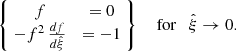
For the second of these, the value −1 was chosen for simplicity, but any other non-zero (finite) value could be imposed instead. Irrespective of the actual value chosen, this condition implies that  as
as  . Hence, f is infinitely steep at the origin, and this family of solutions possesses a singularity there. As for the symmetric case, imposing only the boundary condition at the origin one can find a continuum of solutions which, in most cases, extend to infinity. To extract a set of eigenmodes, i.e. solutions with compact support, an outer boundary condition at a finite location must be imposed; yet, the flux condition and the boundary condition must now be reconsidered for the antisymmetric case. The integration of an antisymmetric solution along the whole real axis naturally yields zero, so that the net magnetic flux automatically vanishes, and the constraint of flux conservation does not lead in this case to a condition for the flux integral on each semi-axis (
 or
or  ). In contrast to the previous cases,
  can now be different from zero for any of the harmonics without violating the condition of flux conservation. We realise, however, that the original boundary conditions (Eq. (41)) at the outer edge must be retained here as well: (a) the search for solutions with compact support leads to the first of those conditions; (b) also, imposing the second of Eq. (41) is just requesting that there is no flux loss nor gain through the outer boundary. This is a reasonable condition to apply not just on mathematical grounds but also through the simple physical consideration that no magnetic flux can be gained from (or lost to) an external unmagnetised domain. Thus, Eq. (41) is used here as outer boundary conditions to define the eigenvalue problem for the antisymmetric case as well. To complete the description, one needs to revisit the normalisation conditions and the evolutionary power laws used for the symmetric case, as follows.
Thus far, we have only presented the obtained solutions for the eigenvalue problem Eq. (45) subject to the boundary conditions appropriate to the antisymmetric case, namely Eqs. (41) and (46). However, ℬ(t) can no longer be determined from the value of the magnetic field at  (which was our choice for the symmetric case), but is here instead dictated by the boundary condition
  as
as  . Using the definition of diffusive flux, Eq. (12) with η = 0 and Eq. (34), and calling (Fd)0(t) = Fd(x → 0, t), we conclude that
 ![Mathematical equation: $ {{{\cal B}}}(t) = [-({{F_{d}}})_0^ (t)\,\chi_a\,{{\cal L}}(t)/H^{1/2}]^{1/3}, $](/articles/aa/full_html/2026/06/aa59489-26/aa59489-26-eq86.gif) with B00 still given by ℬ(t00). The corresponding choice of L002/(χa B002) as a time unit is equivalent, as in Sect. 3.2, to choosing χa = 1 in Eq. (33) and leads to the same equations, Eqs. (35)–(37), for the time-dependence, which contain the essential power laws of the problem.
with B00 still given by ℬ(t00). The corresponding choice of L002/(χa B002) as a time unit is equivalent, as in Sect. 3.2, to choosing χa = 1 in Eq. (33) and leads to the same equations, Eqs. (35)–(37), for the time-dependence, which contain the essential power laws of the problem.
3.4.2. Solutions
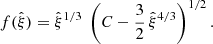
Figure 5 shows the solutions for the first four antisymmetric harmonics. Here, as previously, the term ‘n-harmonic’ refers to a solution with n zeros in the  domain, excluding the outer front. The first harmonic has an exact analytical expression (see Zel’dovich & Barenblatt 1957; Bernis et al. 1993), namely:
 (47)
(47)
To match the boundary condition for the derivative at the centre (Eq. (46), second line), one has to choose C = 32/3, so that
 (48)
(48)
We already came across this solution in a previous step (Eq. (31)), but now we have expressed it in terms of the self-similar variables. As expected, all solutions have infinite slope at the origin, so their numerical integration has to be started using a phase-plane analysis (Moreno-Insertis et al. 2022). The eigenvalue  and other parameters are given in Table 2. Among other things we see that the values for
  for the nth-harmonic here are intermediate between those for the n and n − 1 harmonics for the symmetric case (see Table 1), in agreement with the results of Hulshof (1991). The first harmonic constitutes a particularly good test for MHD codes, since it has an analytical solution and contains a singularity at the origin of type
  , with non-zero diffusive flux, D ≠ 0 (Eq. (34)).
Basic parameters for the first four eigenmodes of the antisymmetric problem.
4. Mode stability: A few time-dependent calculations
In this section, we briefly present a suite of time-dependent numerical solutions of the ambipolar diffusion equation, Eqs. (11) and (12) with η = 0, with various initial conditions. The aim here is to obtain empirical hints on whether the eigenmodes are stable, in the sense that the numerically calculated time-evolution converges to that eigenmode (or not). To that end we use a simple integrator based on the method of lines with second-order spatial derivatives and first-order update in time. This integrator keeps the net flux constant during the integration to machine precision, which turns out to be of interest for the conclusions reached in the following. As seen below, this integrator accurately keeps the shape and time-dependence of the fundamental mode and of the first antisymmetric harmonic (which are stable, as proved in the mathematical literature and explained below) and of the first symmetric harmonic (which is likely to be stable), so it is a good tool for the study undertaken in this section.
4.1. Solutions with a symmetry condition about x = 0
Here the 1D Cartesian case is considered with boundary conditions at the origin that keep the solution symmetric about x = 0. Since all the solutions have compact support, we set minimally invasive boundary conditions at the right-hand boundary, namely,  , which guarantee that the solutions vanish there until the expanding solutions reach the boundary.
4.1.1. Universality of the ZKBP solution for initial conditions that are not in flux balance
Whenever the initial conditions are not in flux balance, so that the net flux does not vanish, we find that the solution tends asymptotically in time to the ZKBP solution for that particular flux. This is expected, since it is the relevant stable solution for the general case of flux cancellation with unequal amounts of flux in the two polarities (see Kamin & Vázquez 1991; Vázquez 2007). This result applies as well when, in the numerical solution, the non-zero net flux is caused by rounding errors in the numerical discretisation: even if one starts with initial conditions in flux balance (Φmag = 0), discretisation of the initial condition leads to a small non-zero net flux, typically 3, 4, or 5 orders of magnitude smaller than the initial unsigned flux. The integrator for these calculations keeps the net flux constant during the integration; so, the tiny initial net flux is maintained, and it plays a negligible role for as long as the unsigned flux of the physical solution is orders of magnitude larger. But the unsigned flux of the eigenmodes continuously decreases in time. Hence, by waiting a sufficiently long time, the initially tiny net flux will start to play a role, and the final outcome will be a ZKBP solution. Yet, this is generally of little physical interest if the time needed to reach such a state is very long, much longer than the other relevant physical timescales. In the following, we therefore disregard the tiny net initial flux, at least for as long as the unsigned flux of the solution is well above it.
4.1.2. Stability of the first symmetric eigenmode
The first symmetric eigenmode is likely to be an attractor for all symmetric solutions with zero net flux and a single internal null point (for a mathematical discussion of various properties of this eigenmode see Bernis et al. 1993 and Hulshof 1991). The experience gained from many numerical solutions carried out in the context of this paper, although insufficient to prove any general mathematical properties, is fully compatible with that hypothesis. For instance, we have tested cases in which, as initial condition at t = 0, the first symmetric eigenmode was used with the addition of a zero-flux finite deviation from it, namely, an ad hoc deviation that, importantly, does not add zeros to the initial function. As apparent in Fig. 6 and the associated animation, the solution quickly converges to the shape of the first symmetric harmonic and remains there as its asymptotic state. For the size and shape of the perturbation used here, by t = 0.21 (log τs = 0.6), the numerical solution and the exact self-similar solution for the first harmonic are virtually indistinguishable in the diagrams, with the height of both diminishing in time, and their spatial extent increasing, according to the self-similar power laws (36)–(37).
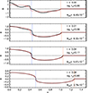 |
Fig. 6. Magnetic field evolution starting from a superposition of the symmetric first harmonic and a zero net-flux finite perturbation which does not add any extra internal null. The panels show four selected instants (top: initial state; bottom: asymptotic evolution). Note the different ranges of the ordinate axes in the different panels. The evolving self-similar first symmetric harmonic is shown as a dashed line in red. The net magnetic flux is Φtot = 7.7 × 10⁻⁶; it does not change during the time evolution. The base-10 logarithm of the diffusive time is indicated. Vertical dashed lines mark locations of the internal zero (blue) and outer front (red) of the solution. An associated animation shows intermediate stages including the solution (upper panel) and the corresponding diffusive flux (lower panel); the associated movie is available online. |
4.1.3. Stability of the higher symmetric harmonics
The stability properties of the higher harmonics do not appear to have been solidly established in the mathematical literature, but to construct such mathematical proofs is outside the scope of the present paper. From our numerical experiments starting with the exact shape of one of the higher harmonics (say, the 6th or the 7th), and so with zero initial flux apart from a tiny rounding error, we observe how, when the spatial resolution is high, they begin by following the exact evolutionary pattern of the harmonic (i.e. maintaining the self-similar shape and following the power laws in time and space corresponding to that harmonic) to high accuracy; however, eventually those solutions deviate from the exact self-similar shape and evolve toward a profile with a single internal null, close to the first symmetric harmonic, with the other internal nulls cancelling in pairs (or being expelled individually through the outer boundary). An example with intermediate resolution is shown in the animation accompanying Fig. 7. The net magnetic flux (which is caused by the numerical discretisation) is −7.4 × 10⁻⁸, i.e. tiny in comparison with the initial unsigned flux 6.5 × 10⁻¹; the deviation from the original self-similar shape caused by the lack of stability of the higher harmonic starts to be apparent at roughly t ≈ 1.5 × 10³, when the unsigned flux has been reduced to ≈1.7 × 10⁻³, which is still four orders of magnitude greater than the net flux. The process of transformation into the first symmetric harmonic takes place starting at that time; to observe that process, we have run the calculation until an advanced time, namely t = 2 × 10¹⁰, when the transformation was clearly complete, and at that point fit the shape of a first symmetric harmonic, for which we know the exact evolution prior and after that time according to the self-similar power laws of Sect. 3.2. Starting at time t = 2.2 × 10⁸, in the animation and in Fig. 7 we have superimposed the shape of that exact self-similar first symmetric harmonic as a dashed cyan curve. We can see how the original solution evolves toward that harmonic, as if the latter were acting as an attractor; in fact, from, roughly, t = 7 × 10⁹ onward the two solutions are indistinguishable in the figure and animation, keeping an excellent fit for the rest of the calculation.
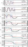 |
Fig. 7. Selected stages in the evolution of the numerical solution of the ambipolar diffusion equation with initial condition having the shape of the seventh symmetric self-similar harmonic and with the numerical mesh containing 2048 grid points. Red: Exact solution for the seventh self-similar harmonic. Black: Actual numerical solution. Cyan (only in the three lowermost panels): exact solution for the first self-similar harmonic that coincides with the numerical solution at the final time calculated in the figure. Note the very different ranges of the ordinate axes in the different panels. Vertical dashed lines: Locations of the internal zeros of the numerical solution (blue); outer front of the exact 7th symmetric self-similar harmonic (red). The total (or net) magnetic flux is −7.4 × 10⁻⁸. An associated animation is provided that shows intermediate stages including the solution (top) and the corresponding diffusive flux (bottom); the associated movie is available online. |
The foregoing can only be taken as a hint of an instability of the higher harmonics and of the suggestion that the first symmetric harmonic acts as an attractor for them. A detailed study, with very high spatial resolution and possibly comparing different numerical methods must be left for future work; exact mathematical proofs, in turn, would need a sophisticated applied mathematics treatment.
4.2. Time evolution with no boundary condition imposed at x = 0 and transforming into the dipole solution
To test empirically for the stability of the first symmetric harmonic subjected to more general perturbations, we extend the initial condition to the negative x-axis but maintain the eigenmode shape with even symmetry for the initial condition. To that shape, perturbations are added of either symmetric or antisymmetric shape to see if the first harmonic is indeed stable. We first report on simple cases, which need not be graphically illustrated: (1) If we just let it go with a very small net flux (arising from numerical rounding errors) but otherwise equal to the first symmetric harmonic, it maintains that shape and obeys the corresponding power laws. (2) If one adds a not necessarily small perturbation with no net flux and which is symmetric about x = 0, the solution quickly converges to the first symmetric harmonic, following the corresponding power laws.
The next case (i.e. case 3) is perhaps less obvious and we illustrate it here with a figure (Fig. 8) and an associated animation. As initial condition (top panel), we take the same first harmonic symmetric about x = 0 as in the previous two cases (dashed red curve), but now add a finite perturbation with an antisymmetric shape (dashed green curve). The solution in time for the superposition is shown as a solid black curve in all panels whereas the corresponding solution of the symmetric self-similar first-harmonic used to build the initial condition is shown as a dashed red line. It is remarkable to see that the solution quickly loses the internal null point on the left as it is ejected through the outer front (panels b and c), and it adopts an antisymmetric shape which eventually behaves in a self-similar fashion; namely, it behaves similarly to the fundamental dipole solution (see panels d, e, and f). In the latter three panels, which are separated by a long time interval (from τs = 1.5 × 10² to τs = 5 × 10³), the time-dependent evolution of the dipole mode that best fits the final value of the solution in that time series is added using a dashed cyan line: as can be seen, at least in the time range τs = 6 × 10² to τs = 5 × 10³, the actual solution and the dipole one are very close to each other; this is true also for the flux, as can be checked in the associated animation.
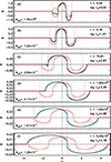 |
Fig. 8. Selected stages in the evolution of the numerical solution described in Sect. 4.2. Panel (a): Initial condition (solid black curve), resulting from the addition of the exact first symmetric self-similar harmonic (dashed red) and a finite antisymmetric perturbation of zero net flux (dashed green). In panels (d)–(f), the exact self-similar dipole harmonic evolving towards the final shape of the numerical solution is superimposed in cyan. Note the different ranges of the ordinate axes in the different panels. An associated animation is provided that shows intermediate stages including the solution (upper panel) and the corresponding diffusive flux (lower panel); the associated movie is available online. |
5. Tests of the Bifrost code and its ambipolar diffusion solver
We have conducted numerical experiments in double precision with the 3D radiation-MHD Bifrost code (Gudiksen et al. 2011) using the ambipolar diffusion solver developed by Nóbrega-Siverio et al. (2020a); the experiments follow a similar procedure to those in Moreno-Insertis et al. (2022). In doing so, we refer here to the solutions derived in the earlier sections of this paper as the theoretical solutions, whereas those calculated with the Bifrost code are referred to as the Bifrost solutions. For brevity, we focus on the symmetric solutions.
As a first step, we would have to consider the fundamental ZKBP solution (Sect. 3.1) shown as the black curve of Fig. 4. This is the most stable of the eigenmodes, and the asymptotic solution for all initial conditions with non-zero flux; also, importantly for the test, it does not have any internal singularity. So, we expect the Bifrost calculation to yield satisfactory results for this solution. Indeed, a first Bifrost test for this eigenmode was already presented in the paper by Nóbrega-Siverio et al. (2020a) with very good results. A far more stringent test for numerical codes is provided by the harmonics to the eigenvalue equation (Eq. (39); or, equivalently, Eq. (45)) found in Sect. 3. The reason for this is the presence of internal current sheets with a finite diffusive flux across them. Since the magnetic field possesses an infinite gradient there, calculating the diffusive flux at such singularities is highly challenging for standard codes, which cannot integrate by going to the phase plane. Here we first show the tests carried out for the first symmetric harmonic (Sect. 5.1) and then those for one of the higher harmonics (Sect. 5.2).
5.1. First symmetric harmonic
The first symmetric harmonic (Sect. 3.1) is shown as the blue curve in Fig. 4. As initial condition for the Bifrost calculation we use that theoretical solution for the right half of the domain centred on an arbitrary coordinate x = (xmax)0, together with its mirror-symmetric counterpart for the left half. At time t = 0, we arbitrarily centre the function at x = (xmax)0 = 2 and locate its outer front at x = 3 on the right and x = 1 on the left, in keeping with the normalisation ℒ(0) = 1 introduced in Sect. 3.2; the function vanishes outside the interval (1, 3) in x. The solution is expected to expand in space according to the rules explained in Sect. 3.2. To cope with that expansion, the integration domain for the numerical calculation is the interval (xL, xR) = (−0.46, 4.66); note that we have set the centre of the function, (xmax)0, on purpose at a location not coinciding with the centre of the numerical grid. At each time-step we calculate the position of the maximum of the numerical solution, xmax(t), and define  . The numerical solution is then compared with the theoretical one for the first harmonic of Sect. 3.3 using the time-dependence (36)–(37),
  , and
, and  .
.
For this test, we used four levels for the spatial resolution, corresponding to nx = 512, 1024, 2048 and 4096 grid cells across the domain. The grid spacing is Δx = 0.01 for the worst resolution and Δx = 0.00125 for the best one. In Fig. 9, the initial function for all the cases is shown in the left panel; the final state at time t = 100 (τs = 1206) for the lowest resolution case (nx = 512) is presented in the middle panel. The theoretical solution for the first harmonic, extended with its mirror-symmetric solution for negative ξ, is superimposed as a thick red curve. By construction, at time t = 0 (left panel) the red and black curves lie exactly on top of each other. In the middle panel, we notice a small mutual deviation at the final time. The absolute value of the relative deviation between the maxima of the theoretical and the Bifrost solutions for each of the resolution levels is shown in the right panel as a function of time. The relative deviation first grows and then stays at a roughly constant level in the advanced stages: this is due to the improvement of spatial resolution that naturally comes about through the expansion of the spatial support of the function as time progresses.
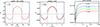 |
Fig. 9. A comparison of the Bifrost runs (black thick curve) with the theoretical solutions (red curves), showing the initial condition (left panel) and the final configuration for nx = 512 (central panel). The relative mutual deviation of the maxima between the theoretical and Bifrost solutions for four resolution levels is given in the right panel. |
Another way of testing the Bifrost solution is to compare with the power laws (36)–(37) for the decay of ℬ and expansion of ℒ given by K and H. Thus, for the first harmonic from Table 1, the exponents of the power laws are α = −0.387 and γ = 0.113. Figure 10 gives a comparison for the worst-resolution case nx = 512 (solid black: Bifrost solution; dashed red: theoretical laws). The left panel gives the comparison for ℬ(t), while the position of the outer front, ℒ(t), and of the internal current sheet, ℒcs(t), are given in the central panel. The a posteriori determination of the location of the outer front is prone to numerical inaccuracies, due to the sharp corner between the solution (which declines as | 2 H δ |1/2; see Sect. 3.3) and the zeros beyond the front. On the other hand, the time-dependent calculation of the location of the current sheets is most demanding for the Bifrost runs, as explained in the preamble to this section. Yet, the figure shows the match between theory and Bifrost results to be excellent: the Bifrost curves agree with those of the theoretical law (36)–(37) with a precision of 5 × 10⁻³ for ℬ(t) (left panel), 2 × 10⁻² (middle panel, ℒ) and 10−2 (middle panel, ℒcs). The highest resolution case (nx = 4096) gives a precision of 7 × 10⁻⁴ for  , 3 × 10⁻³ for ℒ(t), and 2 × 10⁻³ for ℒcs(t), respectively.
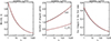 |
Fig. 10. Time-dependence of the maximum of the magnetic field (left panel), the location of the singular points (middle panel; upper curve for ℒ(t), lower curve for ℒcs(t)), and the value of the integral ∫B(x, t) dx in the central lobe of the solution (right panel) for the solution of the first harmonic, illustrated in Fig. 4. The Bifrost solution is shown as a solid black line and the theoretical solutions as dashed red lines. |
The ability of Bifrost to cope with the singularities at the internal current sheets can be further tested by evaluating the integral of the magnetic field in either of the lobes and studying how it varies in time. The integral of the magnetic field between the nulls or between the central maximum and the current sheet must evolve in time exactly as ℬ(t) ℒ(t), i.e. using the analytical laws (37), as a power law of τs(t) with exponent ![Mathematical equation: $ (1-{\hat{K}})/[2(1+{\hat{K}})] $](/articles/aa/full_html/2026/06/aa59489-26/aa59489-26-eq102.gif) . Looking at the value of
. Looking at the value of  in Table 1 for the different harmonics, we see that the integral is conserved in time for the ZKBP solution (
 ) and decreases for any of the other harmonics. For the first harmonic, in particular,
 ![Mathematical equation: $ (1-{\hat{K}})/[2(1+{\hat{K}})] = -0.275 $](/articles/aa/full_html/2026/06/aa59489-26/aa59489-26-eq105.gif) . The comparison between numerical solution and analytical power law appears in the right panel of Fig. 10, again for the worst-resolution case (nx = 512). The power-law exponent of the minimum-square fit to the numerical curve matches the analytical value with a precision 7 × 10⁻³. For nx = 4096, the precision is an order of magnitude better, namely, 9 × 10⁻⁴.
. The comparison between numerical solution and analytical power law appears in the right panel of Fig. 10, again for the worst-resolution case (nx = 512). The power-law exponent of the minimum-square fit to the numerical curve matches the analytical value with a precision 7 × 10⁻³. For nx = 4096, the precision is an order of magnitude better, namely, 9 × 10⁻⁴.
As a final remark, we note that the harmonic used in this section is expected to be stable (as discussed in Sect. 4.1.2). This implies that the solution of the equation, even if with the addition of small zero net-flux perturbations, naturally, i.e. mathematically, tends to the exact harmonic. Still, if the numerical integration at the sharp current sheets were inaccurate, then magnetic flux would be artificially annihilated across them, and the timescale of evolution could deviate importantly from that given by the power laws of Eqs. (36)–(38). Also, depending on the integrator used, the numerical errors could cause an artificial deviation of the net flux from zero. The fact that the fit to the theoretical solution is very good is the best proof of the accuracy of the Bifrost calculation.
5.2. Higher harmonics
Consider the third symmetric harmonic (light-green curve in Fig. 4), which contains six internal nulls (three on each side of the maximum) as well as the two outer fronts. The properties of the theoretical solution (Sect. 3, Table 1) suggest that the decay of the maxima with α = −0.465 is faster than for the fundamental, whereas the spatial expansion is much slower with γ = 3.47 × 10⁻².
The Bifrost solution for the lower resolution case (nx = 512) is shown in Fig. 11, where it can be observed that the deviation from the theoretical solution is more pronounced than for the first symmetric harmonic (Fig. 9). The effective resolution for each lobe is roughly twice as bad as for the first harmonic. The same is true for the corresponding curves for the maxima (right panel of the figure). For the highest resolution case (nx = 4096), the maximum relative deviation is quite small (6 × 10⁻³) but is a factor of 3 larger than for the first harmonic. The low-resolution case gives a relative deviation of several percent, and continuously deteriorates in the right half of the log τs range.
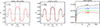 |
Fig. 11. Comparison of the Bifrost solution (black thick curve) for the third harmonic with the theoretical solution (red curve), showing the initial (left) and final (middle) profiles for a resolution of nx = 512. Right panel: Relative mutual deviation of the maxima between the theoretical and Bifrost solutions for the four resolution levels used in the test. |
The location of the zeros and of the corresponding power-law exponents provides a challenging test in the lower resolution case (nx = 512) for the high harmonics. The numerical location of the outer front [ℒ(t)] is found to have a maximum deviation of 2% from the theoretical value, while the fit of ℒ(t) to a power law agrees with the theoretical value to 6%. The situation is more demanding for the innermost current sheet, since, although  is determined numerically with accuracy better than 10%, its fit to a power law produces an exponent that agrees with the theoretical value only within 2 × 10⁻¹. However, the maximum of the solution and the magnetic flux in the innermost lobe yield exponents with an acceptable accuracy of 2 × 10⁻² of the theoretical values. Naturally, the higher resolution cases produce better comparisons between theoretical and numerical variables. The highest resolution case (nx = 4096) gives an accuracy of 3 × 10⁻⁴ for the power-law exponent of the decay of the maximum, 10−2 for the location of the outer front, 10−2 for the location of the innermost current sheet, and 3 × 10⁻⁴ for the integrated flux.
To properly judge the value of the test for this harmonic or higher order ones, one has to take into account that it is unstable (as all harmonics above the first), i.e. prone to decay into the first symmetric harmonic (or the dipole solution, if antisymmetric cases are considered) whenever any zero net-flux deviation is added to it, as can be easily checked using a simple integrator, like that used in Sect. 3. So, the question is: when is that transformation going to take place? If the accuracy of the initial conditions and of the numerical integration were extremely high, one would expect the transformation to occur for very large diffusive times. Indeed, using the integrator of Sect. 3, one sees that the first loss of nulls from the solution (either through merging of pairs of nulls or ejection through the outer boundary) occurs at times t = 2.4 × 10⁷, t = 6.6 × 10⁷, and t = 5.5 × 10⁹ (log τs = 9.0, 9.4, 11.3) for resolutions of, respectively, 1024, 2048 and 4096 cells in the whole domain of integration. So, in a certain sense, this test is more demanding than that for stable harmonics: additionally to the problem of the possible artificial flux annihilation at internal current sheets (see Sect. 5.1), which can modify the time- or length-scales of the solution while preserving the shape of the stable harmonic, the solution here is also intrinsically prone to transformation towards a different harmonic. By the same token, the test in this case consists basically in checking for how long the numerical solution remains in the close neighbourhood of the initial harmonic without any apparent transformation toward the stable lower order harmonic.
6. Discussion
Increasingly, the importance of ambipolar diffusion in the solar atmosphere is being realised and incorporated in advanced multi-dimensional codes such as Bifrost (Martínez-Sykora et al. 2012; Nóbrega-Siverio et al. 2020a), MURaM (Cheung & Cameron 2012; Rempel & Przybylski 2021), MANCHA (Khomenko & Collados 2012; González-Morales et al. 2018), MPI-AMRVAC (Popescu Braileanu & Keppens 2021; Keppens et al. 2023), Lare3D (Chouliaras et al. 2023), NIRVANA (Ziegler 2011), and others. The fact that ambipolar diffusion is a non-linear process leads to much unexpected behaviour that differs from the familiar linear process of Ohmic diffusion. Understanding the physical effects of ambipolar diffusion is therefore of importance, and one way to disclose them is through a study of the pure diffusion problem, as carried out in this paper for the Cartesian case and in our preceding paper (Moreno-Insertis et al. 2022) for the 2D cylindrical case.
6.1. Simple 1D solutions
The importance of singular profiles of B(x)∝x1/3 type has been discussed. For static situations, a central Ohmic-diffusion region resolves the singularity of the field profile near the null point; however, an important realisation by Parker (1963) is that the overall diffusion timescale, the magnetic flux transfer rate toward the null, and also the rate of Ohmic heating are determined not by Ohmic diffusion near the null but by the ambipolar diffusion profile. On the other hand, we have found stagnation-point flow solutions in which an external, pure advection region surrounds an internal ambipolar diffusion region, and the latter contains in its core a small domain dominated by Ohmic diffusivity. Oppositely directed magnetic flux is transported in from large distances first through pure field advection until it reaches the diffusive central region. This consists of: first, an ambipolar-diffusion-dominated domain, with the field steepening to a singular ∝x1/3 profile; then an Ohmic diffusion region, in the immediate surroundings of the central null, where the field is annihilated. The flux transfer rate is uniform throughout the entire domain and, as in the classical stagnation flow problem, it is determined by the value of the electric field.
6.2. Microscopic aspects
Concerning microscopic (i.e. multi-fluid) aspects, a word of caution is necessary when dealing with singular profiles created by ambipolar diffusion effects, especially if the singularities are tied to fixed plasma elements like those of Sect. 2 or the central singularity in the antisymmetric eigenmodes of Sect. 3.4. As discussed by Zweibel (1994) and Brandenburg & Zweibel (1994) for the B(x)∝x1/3 profiles, in those cases, one has to distinguish the bulk plasma speed from the motion of its individual species. In the standard ambipolar-diffusion approach (see Sect. 1), the effect of the Lorentz force on the ions, but not on the neutrals, leads to a mutual drift and to a drift of either of them with respect to the bulk plasma motion; in a 1D situation with  , the latter can be written
 (49)
(49)
In a B ∝ x1/3 profile with zero bulk plasma speed, even if resolved by an Ohmic layer near the null, these drift speeds cause the accumulation of ions (and also the depletion of neutrals) around the null, nearing a singular behaviour if the Ohmic layer is tiny by comparison to the ambipolar-dominated region. This can be a problem when the profile is fixed at the same plasma elements. In standard kinematic models all dynamical considerations are set aside, and, coherently, problems related to accumulation of microscopic particles could also be ignored; nevertheless, this neglect becomes particularly critical in cases when the ambipolar-diffusion-dominated range reaches very close to the singularity. So, while the solutions in this paper and others are of interest when the microscopic aspects can be ignored because the time evolution of the system under consideration renders them unimportant (and, also, as mathematical solutions and as demanding tests for MHD codes), the multi-fluid aspects should be kept in mind in critical situations when near-singularities are reached and maintained at the same plasma elements for timescales comparable to other physical timescales of the problem.
6.3. Self-similar solutions
Self-similar solutions have been studied here in detail, with magnetic fields B(x, t) = g(t)f(ξ) that depend on the spatial coordinate in the combination ξ = x/ℒ(t); they are appropriate when there are no natural length or timescales in the system, so all that can be expected is that the latter fulfill mutual relations like those of Eqs. (36)–(38). The zero-order solution and the first symmetric and antisymmetric harmonics are the basic solutions of the problem. The zero-order solution is the only one with non-zero net flux; the first, or higher, harmonics have as many internal null points in the x ≥ 0 domain as the order of the harmonic. At those internal nulls, positive magnetic flux is brought in toward the null from one side and negative flux from the other, so that flux annihilation ensues. In this way, while the net zero flux of the eigenmode is preserved in the time evolution, the unsigned flux gradually decreases in time toward zero. This annihilation follows from the cancellation of the exponents of B2 and dB/dx in the expression for the flux transfer rate (Eq. (12), with η = 0) for B ∝ x1/3 and is of interest in the absence of any Ohmic diffusion, i.e. from a purely mathematical point of view. In fact, with a small, but non-zero Ohmic dissipation, the annihilation will be Ohmic and take place in the immediate neighbourhood of the null points. Still, the solution outside that neighbourhood will be the exact harmonic of the pure ambipolar diffusion problem.
6.4. Mode stability
We have probed the stability of a few of the eigenmodes through calculations starting with an unperturbed high-order eigenmode, or with a perturbed low-order one. When the net flux of the initial condition is zero, we have seen how the solution evolves toward either the first symmetric harmonic or the dipole solution. Simple cases with non-zero initial net flux lead to the fundamental ZKBP solution with the same net flux: this elementary case has not been illustrated here but has been repeatedly obtained by us in different calculations and is well known from the literature. The cases with zero initial net flux are more interesting. The dipole mode is an attractor; the first symmetric mode is likely to be one but, to our knowledge, this has not yet been fully proved with mathematical tools. What we have obtained here is just an empirical hint, so to say, that the higher order eigenmodes tend to evolve into the first-order harmonics (either the symmetric or antisymmetric one) via cancellation of the internal null points in pairs or ejection of single nulls through the outer boundary; we have also shown, in one of the examples, that an asymmetric perturbation of the first symmetric harmonic can make it turn into the dipole solution asymptotically in time.
6.5. Bifrost and large-code tests
We are proposing that the time evolution of the eigenmodes of the self-similar problem can be used as strong tests for ambipolar diffusion solvers in MHD codes. Given the probably unstable nature of the higher order modes, two types of simple test can be envisaged: either a pure first-order harmonic is verified to maintain its shape in time, according to the self-similar laws, or a higher order harmonic ends up evolving into the first-order eigenmodes asymptotically in time. We carried out both types of tests with the Bifrost code. For the second one (Sect. 5.2), which is less amenable to quantitative evaluation, we have checked the time evolution of the third symmetric harmonic. Here, for a comparatively low-resolution case (nx = 512 cells), the code has kept the 3rd-harmonic appearance at least until t = 100 (log τs = 3.6), with roughly twenty times higher accuracy for nx = 4096 cells. For the first type of test (Sect. 5.1), we have used the first symmetric harmonic as initial condition; in the Bifrost run, the solution maintained its self-similar appearance in time to a high order of accuracy, both concerning the deviation from the exact mathematical solution for it as well as the integral of the flux in its central lobe and the location of the internal nulls. It is worth noting the difficulty of passing this test for the code: in the exact solution, the internal nulls are an essential singularity; in the numerical solution, that singularity will be resolved by ohmic diffusivity (or by the intrinsic numerical diffusivity of the code). The fact that the null and its associated singularity evolve in time in the Bifrost calculation as prescribed by the theoretical solution can be taken as an indicator of the quality of the ambipolar diffusion solver in the code.
7. Conclusions
The main conclusions of this work are as follows:
-
We considered a series of solutions in which an ambipolar diffusion region harbours in its core an Ohmic-diffusion one. In particular, a generalisation of the classical stagnation-point flow has been found with three domains (advection-, ambipolar-, and Ohmic-dominated), where each is contained in the deep interior of the previous one. Flux annihilation takes place in the Ohmic region, but at a rate determined by the advection flow in the external domain and mediated by the ambipolar diffusion region.
-
We calculated the parameters and runs of the eigenmodes for the self-similar solutions of the 1D Cartesian ambipolar diffusion equation, i.e. of the countable subset of self-similar solutions that have compact support. These solutions have been efficiently obtained using phase-plane techniques in spite of the essential singularities they have within their domain. Although their existence had previously been studied in the mathematical literature, their form had not yet been presented.
-
The stability of those eigenmodes has been probed using direct integration of the time-dependent 1D ambipolar diffusion equations. In particular, we have seen that modes with orders above the first (or modes with zero net-flux perturbations) spontaneously evolve into first-order modes. Although this result is not presented as a stability proof in the mathematical sense, it can be used as a strong suggestion (and visualisation) of the unstable nature of higher order modes. On the other hand, the behaviour of the first-order symmetric and antisymmetric eigenmodes in the numerical solutions is consistent with the expectation that they are stable.
-
Tests for the ambipolar diffusion solver in use in the Bifrost code were carried out: one with the first symmetric harmonic and another with a higher order symmetric mode that is expected to spontaneously transform into the first one. The tests were successful. Finally, the usefulness of such tests for other MHD codes was discussed.
The cartesian solutions obtained in this paper complement those presented by Moreno-Insertis et al. (2022) for cylindrical symmetry. Both together can provide fundamental insights into the physical and mathematical nature of the ambipolar diffusion problem and serve as stringent tests of the capabilities of ambipolar diffusion solvers in MHD codes.
Data availability
Movies associated with Figs. 6, 7, and 8 are available at https://www.aanda.org
Acknowledgments
This research has been supported by the European Research Council through the Synergy Grant number 810218 (“The Whole Sun”, ERC-2018-SyG); by the Spanish Ministry of Science, Innovation and Universities through project PGC2018-095832-B-I00; and by the Research Council of Norway (RCN) through its Centres of Excellence scheme, project number 262622. Use of the resources provided by Sigma2 – the National Infrastructure for High Performance Computing and Data Storage in Norway is also acknowledged.
References
- Arber, T. D., Haynes, M., & Leake, J. E. 2007, ApJ, 666, 541 [Google Scholar]
- Arber, T. D., Botha, G. J. J., & Brady, C. S. 2009, ApJ, 705, 1183 [Google Scholar]
- Ballester, J. L., Alexeev, I., Collados, M., et al. 2018, Space Sci. Rev., 214, 58 [Google Scholar]
- Barenblatt, G. 1952, Prikl. Mat. i Mekh, 16, 67 [Google Scholar]
- Bauer, S. J. 1973, Physics of Planetary Ionospheres (Berlin: Springer) [Google Scholar]
- Bernis, F., Hulshof, J., & Vázquez, J. 1993, J. Reine Angew Math., 435, 1 [Google Scholar]
- Braginskii, S. I. 1965, Rev. Plasma Phys., 1, 205 [Google Scholar]
- Brandenburg, A., & Zweibel, E. G. 1994, ApJ, 427, L91 [NASA ADS] [CrossRef] [Google Scholar]
- Cally, P. S., & Khomenko, E. 2018, Astrophys. J., 856, 20 [Google Scholar]
- Cheng, G., Ni, L., Chen, Y., & Lin, J. 2024, A&A, 685, A2 [NASA ADS] [CrossRef] [EDP Sciences] [Google Scholar]
- Cheung, M. C. M., & Cameron, R. H. 2012, ApJ, 750, 6 [NASA ADS] [CrossRef] [Google Scholar]
- Chouliaras, G., Syntelis, P., & Archontis, V. 2023, ApJ, 952, 21 [NASA ADS] [CrossRef] [Google Scholar]
- Cowling, T. 1957, Magnetohydrodynamics (Interscience Publishers), Intersci. Tracts Phys. Astron. [Google Scholar]
- Crutcher, R. M. 1999, ApJ, 520, 706 [NASA ADS] [CrossRef] [Google Scholar]
- De Pontieu, B., Martínez-Sykora, J., & Chintzoglou, G. 2017, ApJ, 849, L7 [Google Scholar]
- Draine, B. T. 1986, MNRAS, 220, 133 [NASA ADS] [Google Scholar]
- Draine, B. T., & McKee, C. F. 1993, Ann. Rev. Astron. Astrophys., 31, 373 [Google Scholar]
- González-Morales, P. A., Khomenko, E., Downes, T. P., & de Vicente, A. 2018, A&A, 615, A67 [Google Scholar]
- Goodman, M. L. 2000, Astrophys. J., 533, 501 [Google Scholar]
- Goodman, M. L. 2004, Astron. Astrophys., 416, 1159 [Google Scholar]
- Grundy, R. 1979, Q. Appl. Math., 37, 259 [Google Scholar]
- Gudiksen, B. V., Carlsson, M., Hansteen, V. H., et al. 2011, A&A, 531, A154 [NASA ADS] [CrossRef] [EDP Sciences] [Google Scholar]
- Heitsch, F., & Zweibel, E. G. 2003, ApJ, 583, 229 [NASA ADS] [CrossRef] [Google Scholar]
- Hennebelle, P., & André, P. 2013, Astron. Astrophys., 560, A68 [Google Scholar]
- Hillier, A. 2019, Phys. Plasmas, 26, 082902 [Google Scholar]
- Hillier, A. S. 2024, Philos. Trans. R. Soc. Lond. Ser. A, 382, 20230229 [Google Scholar]
- Hillier, A. S., Snow, B., & Luna, M. 2024, Philos. Trans. R. Soc. Lond. Ser. A, 382, 20230230 [Google Scholar]
- Hulshof, J. 1991, J. Math. Anal. Appl., 157, 75 [Google Scholar]
- Kamin, S., & Vázquez, J. 1991, SIAM J. Math. Anal., 22, 34 [Google Scholar]
- Keppens, R., Popescu Braileanu, B., Zhou, Y., et al. 2023, A&A, 673, A66 [NASA ADS] [CrossRef] [EDP Sciences] [Google Scholar]
- Khomenko, E., & Collados, M. 2012, Astrophys. J., 747, 87 [Google Scholar]
- Khomenko, E., Díaz, A., de Vicente, A., Collados, M., & Luna, M. 2014, Astron. Astrophys., 565, A45 [Google Scholar]
- Khomenko, E., Collados, M., & Díaz, A. J. 2016, Astrophys. J., 823, 132 [Google Scholar]
- Khomenko, E., Vitas, N., Collados, M., & de Vicente, A. 2018, A&A, 618, A87 [NASA ADS] [CrossRef] [EDP Sciences] [Google Scholar]
- Kumar, N., & Roberts, B. 2003, Sol. Phys., 214, 241 [Google Scholar]
- Kunz, M. W., & Mouschovias, T. C. 2010, MNRAS, 408, 322 [NASA ADS] [CrossRef] [Google Scholar]
- Leake, J. E., & Arber, T. D. 2006, Astron. Astrophys., 450, 805 [Google Scholar]
- Leake, J. E., & Linton, M. G. 2013, Astrophys. J., 764, 54 [Google Scholar]
- Leake, J. E., Lukin, V. S., Linton, M. G., & Meier, E. T. 2012, Astrophys. J., 760, 109 [Google Scholar]
- Leake, J. E., Lukin, V. S., & Linton, M. G. 2013, Phys. Plasmas, 20, 061202 [NASA ADS] [CrossRef] [Google Scholar]
- Li, Z.-Y., Banerjee, R., Pudritz, R. E., et al. 2014, Protostars and Planets VI, 173 [Google Scholar]
- Mac Low, M.-M., & Klessen, R. S. 2004, Rev. Mod. Phys., 76, 125 [Google Scholar]
- Martínez-Sykora, J., De Pontieu, B., & Hansteen, V. 2012, Astrophys. J., 753, 161 [Google Scholar]
- Martínez-Sykora, J., De Pontieu, B., Carlsson, M., et al. 2017a, Astrophys. J., 847, 36 [Google Scholar]
- Martínez-Sykora, J., De Pontieu, B., Hansteen, V. H., et al. 2017b, Science, 356, 1269 [Google Scholar]
- Martínez-Sykora, J., De Pontieu, B., De Moortel, I., Hansteen, V. H., & Carlsson, M. 2018, ApJ, 860, 116 [Google Scholar]
- Martínez-Sykora, J., Leenaarts, J., De Pontieu, B., et al. 2020, ApJ, 889, 95 [Google Scholar]
- Mestel, L., & Spitzer, L. 1956, MNRAS, 116, 503 [NASA ADS] [CrossRef] [Google Scholar]
- Mitchner, M., & Kruger, C. H. 1973, Partially Ionized Gases (Wiley), Wiley Ser. Plasma Phys. [Google Scholar]
- Moreno-Insertis, F., Nóbrega-Siverio, D., Priest, E. R., & Hood, A. W. 2022, Astron. Astrophys., 662, A42 [Google Scholar]
- Mouschovias, T. C., & Paleologou, E. V. 1979, ApJ, 230, 204 [NASA ADS] [CrossRef] [Google Scholar]
- Nakamura, F., & Li, Z.-Y. 2008, ApJ, 687, 354 [NASA ADS] [CrossRef] [Google Scholar]
- Ni, L., Kliem, B., Lin, J., & Wu, N. 2015, ApJ, 799, 79 [Google Scholar]
- Ni, L., Lin, J., Roussev, I. I., & Schmieder, B. 2016, ApJ, 832, 195 [Google Scholar]
- Ni, L., Cheng, G., & Lin, J. 2022, A&A, 665, A116 [NASA ADS] [CrossRef] [EDP Sciences] [Google Scholar]
- Nóbrega-Siverio, D., Martínez-Sykora, J., Moreno-Insertis, F., & Carlsson, M. 2020a, A&A, 638, A79 [EDP Sciences] [Google Scholar]
- Nóbrega-Siverio, D., Moreno-Insertis, F., Martínez-Sykora, J., Carlsson, M., & Szydlarski, M. 2020b, A&A, 633, A66 [NASA ADS] [CrossRef] [EDP Sciences] [Google Scholar]
- Parker, E. N. 1963, Astrophys. J. Suppl, 8, 177 [Google Scholar]
- Parker, E. 1973, J. Plasma Phys., 9, 49 [Google Scholar]
- Pattle, R. E. 1959, Q. J. Mech. Appl. Math., 12, 407 [CrossRef] [Google Scholar]
- Pfaff, R. F. 2012, Space Sci. Rev., 168, 23 [Google Scholar]
- Popescu Braileanu, B., & Keppens, R. 2021, A&A, 653, A131 [NASA ADS] [CrossRef] [EDP Sciences] [Google Scholar]
- Priest, E. 1982, Solar Magnetohydrodynamics (Dordrecht: D. Reidel) [Google Scholar]
- Priest, E. R. 2014, Magnetohydrodynamics of the Sun (Cambridge, UK: Cambridge University Press) [Google Scholar]
- Rempel, M., & Przybylski, D. 2021, ApJ, 923, 79 [NASA ADS] [CrossRef] [Google Scholar]
- Ruderman, M. S., Ballai, I., Khomenko, E., & Collados, M. 2018, Astron. Astrophys., 609, A23 [Google Scholar]
- Sakai, J. I., & Smith, P. D. 2009, ApJ, 691, L45 [Google Scholar]
- Shu, F. H. 1983, ApJ, 273, 202 [NASA ADS] [CrossRef] [Google Scholar]
- Snow, B., Botha, G. J. J., McLaughlin, J. A., & Hillier, A. 2018, A&A, 609, A100 [NASA ADS] [CrossRef] [EDP Sciences] [Google Scholar]
- Soler, R., Oliver, R., & Ballester, J. L. 2010, Astron. Astrophys., 512, A28 [Google Scholar]
- Soler, R., Díaz, A. J., Ballester, J. L., & Goossens, M. 2012, ApJ, 749, 163 [NASA ADS] [CrossRef] [Google Scholar]
- Sonnerup, B., & Priest, E. 1975, J. Plasma Phys., 14, 283 [Google Scholar]
- Spitzer, L. 1962, Physics of Fully Ionized Gases (New York: Interscience) [Google Scholar]
- Tritsis, A. 2025, A&A, 700, A152 [NASA ADS] [CrossRef] [EDP Sciences] [Google Scholar]
- Vázquez, J. 2007, The Porous Medium Equation. Mathematical Theory (Oxford: Clarendon Press), Oxford Math. Monogr. [Google Scholar]
- Vranjes, J., Poedts, S., Pandey, B. P., & De Pontieu, B. 2008, Astron. Astrophys., 478, 553 [Google Scholar]
- Wargnier, Q. M., Martínez-Sykora, J., Hansteen, V. H., & Pontieu, B. D. 2022, ApJ, 933, 205 [NASA ADS] [CrossRef] [Google Scholar]
- Zaqarashvili, T. V., Khodachenko, M. L., & Rucker, H. O. 2011, Astron. Astrophys., 529, A82 [Google Scholar]
- Zel’dovich, Y. B., & Barenblatt, G. 1957, Appl. Math. Mech., 21, 718 [Google Scholar]
- Zel’dovich, Y. B., & Kompaneets, A. 1950, in Collection of Papers Dedicated to the 70th Birthday of A.F.Ioffe, ed. P. I. Lukirskii (Moscow: Izd. Akad. Nauk. USSR), 61 [Google Scholar]
- Zel’dovich, Y. B., & Raizer, Y. P. 1967, Physics of Shock Waves and High-temperature Hydrodynamic Phenomena (New York: Academic Press) [Google Scholar]
- Ziegler, U. 2011, J. Comput. Phys., 230, 1035 [NASA ADS] [CrossRef] [Google Scholar]
- Zweibel, E. G. 1989, Astrophys. J., 340, 550 [Google Scholar]
- Zweibel, E. G. 1994, NATO ASI Ser. C, 422, 73 [Google Scholar]
- Zweibel, E. G., & Brandenburg, A. 1997, Astrophys. J., 478, 563 [Google Scholar]
- Zweibel, E. G., & Yamada, M. 2009, Ann. Rev. Astron. Astrophys., 47, 291 [Google Scholar]
All Tables
All Figures
|
Fig. 1. Sketch of the solution for steady-state ambipolar diffusion joining B = B1 at x = −L0 to B = B0 at x = L0 for three different values of B1, namely, 2B0/3 (top curve), −2B0/3 (middle curve), and −B0 (bottom curve). |
| In the text | |
|
Fig. 2. Solution to the mixed Ohmic and ambipolar diffusion problem of Eqs. (11) and (12), in which the inset shows the whole range −L0 ≤ x ≤ L0) and the main frame shows just the central domain −0.018L0 ≤ x ≤ 0.018L0)]. Green: Exact solution (16). Blue: Purely ambipolar solution (17). Dashed red: Linear, purely Ohmic solution with slope at the origin equal to that of the full solution (19). Pink: Linear purely Ohmic solution linking the points ( − L0, −B0) and (L0, B0). The dotted vertical lines mark the locations x = ±ld. The blue and green curves and the red segment appear superimposed in the inset. |
| In the text | |
|
Fig. 3. Top: Schematic of a stagnation-point flow configuration, showing magnetic field lines (light-headed arrows) for a 1D current sheet together with a stagnation-point flow (solid-headed arrows). The ideal, ambipolar, and Ohmic regions are indicated. Middle and bottom: Solution of the dimensionless stagnation flow equation (Eq. (29)) with logarithmic (middle panel) and linear axes (bottom panel). Solid red: solution for |
| In the text | |
|
Fig. 4. Top: Fundamental (i.e. ZKBP) and first four symmetric harmonics as functions of the stretched coordinate |
| In the text | |
|
Fig. 5. Top: Fundamental (i.e. dipole) and first three antisymmetric harmonics as functions of the stretched coordinate |
| In the text | |
|
Fig. 6. Magnetic field evolution starting from a superposition of the symmetric first harmonic and a zero net-flux finite perturbation which does not add any extra internal null. The panels show four selected instants (top: initial state; bottom: asymptotic evolution). Note the different ranges of the ordinate axes in the different panels. The evolving self-similar first symmetric harmonic is shown as a dashed line in red. The net magnetic flux is Φtot = 7.7 × 10⁻⁶; it does not change during the time evolution. The base-10 logarithm of the diffusive time is indicated. Vertical dashed lines mark locations of the internal zero (blue) and outer front (red) of the solution. An associated animation shows intermediate stages including the solution (upper panel) and the corresponding diffusive flux (lower panel); the associated movie is available online. |
| In the text | |
|
Fig. 7. Selected stages in the evolution of the numerical solution of the ambipolar diffusion equation with initial condition having the shape of the seventh symmetric self-similar harmonic and with the numerical mesh containing 2048 grid points. Red: Exact solution for the seventh self-similar harmonic. Black: Actual numerical solution. Cyan (only in the three lowermost panels): exact solution for the first self-similar harmonic that coincides with the numerical solution at the final time calculated in the figure. Note the very different ranges of the ordinate axes in the different panels. Vertical dashed lines: Locations of the internal zeros of the numerical solution (blue); outer front of the exact 7th symmetric self-similar harmonic (red). The total (or net) magnetic flux is −7.4 × 10⁻⁸. An associated animation is provided that shows intermediate stages including the solution (top) and the corresponding diffusive flux (bottom); the associated movie is available online. |
| In the text | |
|
Fig. 8. Selected stages in the evolution of the numerical solution described in Sect. 4.2. Panel (a): Initial condition (solid black curve), resulting from the addition of the exact first symmetric self-similar harmonic (dashed red) and a finite antisymmetric perturbation of zero net flux (dashed green). In panels (d)–(f), the exact self-similar dipole harmonic evolving towards the final shape of the numerical solution is superimposed in cyan. Note the different ranges of the ordinate axes in the different panels. An associated animation is provided that shows intermediate stages including the solution (upper panel) and the corresponding diffusive flux (lower panel); the associated movie is available online. |
| In the text | |
|
Fig. 9. A comparison of the Bifrost runs (black thick curve) with the theoretical solutions (red curves), showing the initial condition (left panel) and the final configuration for nx = 512 (central panel). The relative mutual deviation of the maxima between the theoretical and Bifrost solutions for four resolution levels is given in the right panel. |
| In the text | |
|
Fig. 10. Time-dependence of the maximum of the magnetic field (left panel), the location of the singular points (middle panel; upper curve for ℒ(t), lower curve for ℒcs(t)), and the value of the integral ∫B(x, t) dx in the central lobe of the solution (right panel) for the solution of the first harmonic, illustrated in Fig. 4. The Bifrost solution is shown as a solid black line and the theoretical solutions as dashed red lines. |
| In the text | |
|
Fig. 11. Comparison of the Bifrost solution (black thick curve) for the third harmonic with the theoretical solution (red curve), showing the initial (left) and final (middle) profiles for a resolution of nx = 512. Right panel: Relative mutual deviation of the maxima between the theoretical and Bifrost solutions for the four resolution levels used in the test. |
| In the text | |
Current usage metrics show cumulative count of Article Views (full-text article views including HTML views, PDF and ePub downloads, according to the available data) and Abstracts Views on Vision4Press platform.
Data correspond to usage on the plateform after 2015. The current usage metrics is available 48-96 hours after online publication and is updated daily on week days.
Initial download of the metrics may take a while.