


| Issue |
A&A
Volume 710, June 2026
|
|
|---|---|---|
| Article Number | A280 | |
| Number of page(s) | 13 | |
| Section | Stellar structure and evolution | |
| DOI | https://doi.org/10.1051/0004-6361/202659320 | |
| Published online | 19 June 2026 | |
Wide B-type hot subdwarf binaries
I. Orbital and atmospheric parameters
1
Institut für Physik und Astronomie, Universität Potsdam, Karl-Liebknecht-Str. 24/25, 14476 Golm, Germany
2
Dpto. Química “Prof. José Carlos Vílchez Martín”, Facultad de CC Experimentales, Universidad de Huelva, 21007 Huelva, Spain
3
Astronomical Institute of the Czech Academy of Sciences, CZ-25165 Ondřejov, Czech Republic
4
School of Physics and Astronomy, Monash University, Clayton, Victoria 3800, Australia
5
ARC Centre of Excellence for Gravitational Wave Discovery – OzGrav, Clayton, Victoria 8300, Australia
6
Instituto de Física y Astronomía, Universidad de Valparaíso, Gran Bretaña 1111, Playa Ancha, Valparaíso, 2360102, Chile
★ Corresponding author: This email address is being protected from spambots. You need JavaScript enabled to view it.
Received:
4
February
2026
Accepted:
4
May
2026
Abstract
Context. Long-period binary systems containing a B-type hot subdwarf (sdB) and a main sequence (MS) companion are thought to originate from binary interactions involving stable mass transfer from the red giant, which is the progenitor of the sdB, to the MS companion. However, despite the recent progress in modelling their population, some of their observed properties are not fully understood. Because the determination of their orbits requires extended campaigns of high-resolution spectroscopic observations, there have only been a limited number of long-period sdB binaries with completely determined orbital parameters studied thus far.
Aims. We aim to expand the current sample of long-period sdB binaries with fully determined orbital parameters through the analysis of high-resolution spectroscopic data. In addition, we analyse the atmospheric parameters of the cool companions. Increasing the number of well-characterised systems will provide valuable insights into their formation channels and main characteristics.
Methods. A sample of 32 wide binary systems containing sdB stars was selected for the analysis of the radial velocity (RV) curves of both companions. The dataset consisted of high-resolution spectra obtained with the HERMES and UVES spectrographs. The orbital parameters were derived by simultaneously fitting Keplerian orbits to the RVs of the sdB and its companion. The atmospheric parameters of the cool companions were determined using the GSSP code, which analyses the master spectra of the systems with a grid of local thermal equilibrium (LTE) atmospheric models. An additional sample of wide sdB binaries was built by cross-matching the Gaia NSS catalogue with literature catalogues of sdB candidates and spectroscopically confirmed sdB systems. The outcomes from both samples were compared with existing theoretical models to assess their consistency with current formation and evolutionary scenarios.
Results. We obtained complete orbital solutions for 32 wide sdB binaries. The orbital period distribution of the ground-based spectroscopic sample is in reasonable agreement with population-synthesis predictions, except for two outliers. The CMD further suggests that current models overpredict systems with the coolest companions, since the observed systems with BP − RP > 0.3 are associated with companions hotter than 6000 K. The observed period-mass ratio distribution is consistent with recent population synthesis predictions and suggests that the unexplained second branch found in these models is mainly populated by old systems. Setting aside the two long-period outliers, we find the data do not support a clear increase in eccentricity with orbital period, whereas the Gaia-based candidate sample displays a discrepant behaviour, owing to selection effects and larger uncertainties.
Key words: binaries: spectroscopic / stars: evolution / stars: fundamental parameters / subdwarfs
© The Authors 2026
 Open Access article, published by EDP Sciences, under the terms of the Creative Commons Attribution License (https://creativecommons.org/licenses/by/4.0), which permits unrestricted use, distribution, and reproduction in any medium, provided the original work is properly cited.
This article is published in open access under the Subscribe to Open model. This email address is being protected from spambots. You need JavaScript enabled to view it. to support open access publication.
1. Introduction
Binary interactions and mass transfer processes lead to the formation of numerous types of post-interaction binaries, including hot subdwarf B (sdB) stars, which populate the extreme horizontal branch (EHB). These sdB stars are classically described as core-helium-burning objects with a thin hydrogen envelope (approximately 0.01 M⊙) and a mass near the canonical core-helium-flash value of 0.47 M⊙ (Saffer et al. 1994; Brassard et al. 2001; Heber 2009, 2016), although the actual mass range is likely broader (Arancibia-Rojas et al. 2024). They are characterised by high effective temperatures (20 000–40 000 K) and surface gravities typically ranging from 5.0 to 6.0 dex. In the classical scenario, an sdB star forms from the progenitor that had lost most of its hydrogen envelope near the tip of the red giant branch (RGB) and ignited the core through a helium flash (e.g. Heber 2016).
It is now widely accepted that all sdB stars form exclusively through binary interactions (Heber 2016; Pelisoli et al. 2020), as initially suggested by the early work of Mengel et al. (1975). The three primary formation channels proposed to date are: the common-envelope (CE) ejection channel (Paczynski 1976; Han et al. 2002), the stable Roche-lobe overflow (RLOF) channel (Han et al. 2000, 2002), and the formation of a single sdB star through the merger of two helium white dwarfs (WDs; Webbink 1984).
The RLOF channel can form long-period sdB binaries with orbital periods exceeding 500 days, typically containing main sequence (MS) stars as cool companions (Vos et al. 2020). Observations of such systems have been first reported in the past decade (Østensen & Van Winckel 2012; Deca et al. 2012; Vos et al. 2012). In particular, some observed orbital periods surpassed the predictions of existing binary population synthesis (BPS) models (Han et al. 2002, 2003), highlighting the need for an updated theoretical framework. Subsequently, Chen et al. (2013) proposed an atmospheric RLOF model to explain periods of up to 1600 days.
The most recent modelling showed good agreement with the observed formation rates, orbital periods, mass ratios, and metallicities of the wide composite sdB population (Vos et al. 2020). However, some relevant features of these systems are not entirely explained by the models to date. A notable case is the eccentricity at long orbital periods. The work of Vos et al. (2015) proposed a theoretical framework to address this issue, based on the combination of two eccentricity pumping mechanisms: phase-dependent RLOF and a circumbinary (CB) disc. Despite this, the model falls short in reproducing the observed trend in longer orbital periods and is unable to predict the eccentricity of the systems. Increasing the number of accurately determined orbital parameters for long-period sdB binaries will help constrain our understanding of their formation, properties, and evolution.
This paper is organised as follows. Section 2 describes the main characteristics of the wide sdB binary samples used in this work and summarises the observational data, based on either ground-based instruments or Gaia. Section 3 outlines the determination of the orbital solutions and parameters for both samples. The analysis of the atmospheric parameters of the cool companions in wide sdB systems is presented in Sect. 4. Section 5 provides the information on the Galactic orbits and kinematics derived parameters of the systems. Section 5.2 establishes the main parameter relations and compares the results with the current theoretical models. A discussion on the possible causes of agreement or disagreement between observations and models is offered in Sect. 6. Finally, Sect. 7 summarises the main findings and conclusions of this work.
2. Sample and observations
Two different samples of wide sdB binaries are considered in this paper. The first consists of known sdBs that are part of our long-term observing program. Their collection of high-resolution spectra spans more than fifteen years and involves observations from the MERCATOR telescope at the Roque de los Muchachos Observatory (La Palma, Canary Islands, Spain; Gorlova et al. 2013; Vos et al. 2012, 2013, 2017). The program was extended to cover southern targets using the Very Large Telescope at Paranal Observatory (VLT; Atacama Desert, Chile; Vos et al. 2018, 2019). The second sample consists of wide sdB binaries observed by Gaia (Gaia Collaboration 2023b), for which orbital solutions have been derived from either radial velocity spectrometer (RVS) data or astrometric measurements. The subsequent sections outline the target selection criteria and the observational data for both samples.
2.1. Ground-based sample
This sample consists of known wide sdB binaries whose spectral data were obtained with HERMES (High Efficiency and Resolution Mercator Echelle Spectrograph) at the Mercator telescope and with the Ultraviolet and Visual Echelle Spectrograph (UVES) at the VLT. The target candidates were selected from a multitude of low- and medium-resolution spectroscopic and photometric surveys, including but not limited to Green et al. (1986), Downes (1986), Kilkenny et al. (1988), Stark & Wade (2003), and Rhee et al. (2006), Wade et al. (2006). The first target selection was performed using the original hot subdwarf database compiled by Østensen (2006), which contains more than 2300 stars. The target list was updated when new bright sdB/Os were found in later surveys. The original surveys and their more recent follow-up observing campaigns have been consolidated in the hot subdwarf catalogues of Geier et al. (2017), Geier (2020), and Culpan et al. (2022).
The final targets were selected based on their magnitude. The northern hemisphere targets with a limiting magnitude of 11.5 in the V band were observed with HERMES, while in the southern hemisphere, targets up to V = 14 were included, since a larger telescope was used. Binarity was determined based on radial velocity (RV) variations in the data and spectra. HERMES targets were followed for at least two years before determining binarity, usually involving more than ten observations. The UVES targets were followed over the course of two observing seasons (6–12 months), discarding sources that did not display any significant variation from the sample.
HERMES is a high-resolution spectrograph mounted on the 1.2 m Mercator Telescope at the Roque de los Muchachos Observatory in La Palma, Spain. It has a spectral resolution of R = 85 000, and covers a spectral range from 377 to 900 nm (Raskin et al. 2011). It is designed for precise spectroscopic studies of stars managed under conditions of high wavelength stability.
Ten targets were observed with HERMES between 2009 and 2017: eight sdBs and two long-period binaries containing an evolved O-type hot subwarf (sdO). A detailed discussion of the HERMES observations can be found in Vos et al. (2017) for the sdB binaries and Molina et al. (2022) for the sdO ones, along with technical information regarding the spectrograph capabilities. The HERMES sample was completed and no new data have been obtained since then.
UVES is a high-resolution spectrograph installed on the 8.2 m VLT at the Paranal Observatory in Chile. UVES is a two-arm cross-dispersed echelle spectrograph, which was used in standard dichroic-2 437+760 mode, covering a wavelength range of 373–499 nm in the BLUE arm and 565–946 nm in the RED arm. The resolutions achieved for each arm, using a slit width of 1 arcsecond, are R = 41 000 and 42 000, respectively. The spectrograph is designed to study the chemical composition, kinematics, and physical conditions of astronomical objects. The complete set of observations by HERMES and UVES is summarised in Table A.1.
So far, the sample of wide hot subdwarf binaries contains 32 systems whose orbits have been fully solved. Their Galactic locations and colour-magnitude diagram (CMD) are shown in Fig. 1. The GaiaG absolute magnitude is derived from the Gaia apparent magnitude (g) listed in Gaia DR3 according to
 (1)
(1)
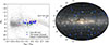 |
Fig. 1. Left: CMD presented by Pelisoli et al. (2020) for their composite hot subdwarf sample is shown as dimmed red diamonds, representing systems whose light curves and rotation periods were studied by the authors. We included the wide hot sdB binary ground-based sample with fully solved orbital parameters as blue filled circles. The Gaia-based sample is shown as green empty diamonds. Interstellar extinctions for both, ground- and Gaia-based samples, are not corrected. Stars catalogued by Geier (2020) as hot subdwarfs are represented as dark gray open circles. MS stars and stars in other evolutionary stages within the region by Lindegren et al. (sample C; 2018) are shown as pale gray dots. Right: Aitoff projection displaying the Galactic coordinates of the wide hot sdB sample. Galactic longitude increases from the centre toward the left, with increments of 30° per tick. Same colour-coded wide sdB systems are shown. |
In the CMD, the sample occupies the extended region populated by hot subdwarf binary systems, located in redder colours than the EHB overdensity of single hot subdwarfs. However, one system in the sample is significantly shifted: BD-07 5977. The cool companion of this system was previously studied and reported as a subgiant star (Vos et al. 2017).
2.2. Gaia sample
The non-single star catalogue from Gaia DR3 (NSS1; Gaia Collaboration 2023a) gathers the sources whose observations are assumed to be non-constant in one of the three channels of observation capabilities from the Gaia probe: astrometric, spectroscopic, and photometric. This has led to a need for different approaches and binary orbit models to obtain their orbital parameters2.
The data release 3 (DR3) catalogues3 by Culpan et al. (2022) contain 6616 hot subdwarfs with spectroscopic confirmation and a further 61 585 hot subdwarf candidates based on Gaia eDR3. They include multi-band photometry and Gaia eDR3 astrometry, as well as classifications based on spectroscopy and colours.
The cross-matching using TOPCAT4 (Taylor 2005) between both the NSS and Culpan et al. (2022) catalogues yields the coincidence of 13 sources. The fundamental data pertaining to the sources and their observations are listed in Table A.1, along with the wide sdB binary systems. Likewise, their CMDs are shown in Fig. 1 (left panel), along with their Galactic coordinates (right panel).
3. Orbital parameters
3.1. Radial velocities
The RVs of the cool companion can be determined using a cross-correlation (CC). The wavelength intervals used avoid telluric lines and those from the hot companion. They represent a good compromise between the high signal-to-noise ratio (S/N) and the low flux contribution of the hot component. Then, the lines of the cool companion within these intervals can be cross-correlated against a high-resolution synthetic template with atmospheric parameters of a similar photometric class to the companion. Before the CC, the synthetic spectrum is convolved to reproduce the line broadening profile of the cool companion star due to the rotational velocity.
The masks utilised for the HERMES spectra are provided by its hermesVR pipeline5. Meanwhile, for UVES spectra, Kurucz LTE synthetic templates were used (Kurucz 1979). The RV error intervals were obtained by performing a Monte Carlo (MC) simulation for each spectrum. Firstly, Gaussian noise was added to the spectrum, based on the continuum noise level in the used wavelength ranges. Then, the synthetic spectrum was employed in a new CC and the final error was calculated from the standard deviation of the RV results from 500 simulations.
The hot sdB stars pose a greater challenge for determining their RVs due to the limited number of available lines. In many cases, only the not blended He Iλ 5876 Å line can be used. However, some systems show a few sharp metal lines originating from the sdB companion. In such cases, the intervals containing those lines were used.
For the hot sdB stars, we employed a custom high-resolution template spectrum. The templates were generated using the XTGRID code (Németh et al. 2012; Nemeth 2019). The code uses a wavelength space direct spectral decomposition (Simon & Sturm 1994) to produce synthetic composite spectra through a linear combination of non-LTE (TLUSTY, Hubeny & Lanz 2017) and LTE (ATLAS, Bohlin et al. 2017) atmosphere models. The process involves an iterative fitting routine to the observed spectrum to determine the main parameters of both the hot and cool companions. To obtain basic templates efficiently and avoid a time-consuming procedure, the initial rough fits to the observed spectra were used as templates for CC. This approach works since, for the CC, the exact line shape is less important than the presence of the respective lines. The RV error intervals were determined using the MC simulations as described above. In Table B.1 we indicate the intervals and/or the specific lines used for the CC of the MS and sdB companions.
3.2. Keplerian fits and orbital parameters
The orbital parameters were obtained by simultaneously fitting Keplerian orbits to RVs of the companions (Hilditch 2001) with eight free parameters: orbital period (P), time of periastron (T0), eccentricity (e), angle of periastron (ω), two semi-amplitudes (K1 and K2), and two systemic velocities (γ1 and γ2). The systemic velocities of both components were considered as separate parameters, since the difference in the surface gravity between the components can cause a line-shift (gravitational redshift; see e.g. Vos et al. 2012, 2013).
The error intervals on the orbital parameters were calculated using an MC approach. In each iteration, each single RV measurement was randomly sampled using a normal distribution centred on its best value and a standard deviation equal to its standard error. The final orbital parameters are the mean values of 1000 iterations, while their standard deviations were used as the error intervals.
Figure 2 shows an example of RVs and the simultaneously Keplerian orbits fitted to the companions of the PG1514+034 system. Table B.2 presents the orbital parameters obtained from the corresponding solutions for the sample of wide sdB binaries.
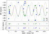 |
Fig. 2. RV curves and residuals for PG1514+034. The RVs of the cool companion are plotted as green filled circles, while those of the sdB companion are shown as blue filled squares. RV error bars (1σ), obtained through MC simulations, are included. The best-fit Keplerian orbits, simultaneously fitted for both the MS and sdB companions, are represented by a solid line for the cool companion and a dotted line for the hot one. |
3.3. Gaia-based orbital solutions
The orbital periods and eccentricities of the wide sdB systems whose orbital solutions were determined by Gaia are shown in Table 1. The data are obtained from the astrometric and photometric channels of Gaia. The Gaia orbital solutions for the sample (for all but one system) are provided by the model for an astrometric binary source compatible with Campbell orbital elements (Halbwachs et al. 2023). The so-called elements involve the semi-major axis of the orbit described by the photocentre, a0, the inclination of the orbital plane with respect to the sky, i, the position angle of the ascending node, Ω, and the periastron longitude measured from the ascending node, ω. The measurement of the position of the photocentre relative to the barycentre of the system is related to these elements by a completely non-linear relationship. The solutions of these elements are obtained by applying the formulas provided by Binnendijk (1960) or Halbwachs et al. (2023).
Orbital parameters from Gaia-based solutions (NSS) for the Gaia-based sample.
The RA and Dec coordinates and parallaxes (distances) of the ground-based sample are provided from Gaia DR3. In contrast, for the Gaia sample, the solutions are from the NSS, since they are expected to supersede the original ones in Gaia DR3 (Gaia Collaboration 2023a). Hence, they are used in Table 1. A detailed description of this solution approach and its constraints is included in the documentation provided on the Gaia-ESA Web6.
Orbital parameters for the Gaia DR3 system 4850445797329363328 were derived from its single-lined spectroscopic data (SB1) from the Gaia spectroscopic channel. Following a methodology similar to that described in the previous subsection in relation to the SB2 spectra of the wide sdB sample, the RVs were fitted using a Keplerian orbit to determine the key orbital parameters of the observed component (Gosset et al. 2025): orbital period (P), time of periastron passage (T0), eccentricity (e), argument of periastron (ω), RV semi-amplitude (K), and systemic RV (γ). The RV curve is fitted using a general Keplerian function via a least-squares optimisation procedure. The quality of the fit is assessed using the reduced chi-squared (χ2) statistic. A detailed description of the fitting process in SB1 and its constraints is available in the Gaia-ESA documentation7.
4. Atmospheric parameters of the cool companions
We studied the composite master spectra of the cool companion stars to derive their atmospheric parameters. They were created by shifting the spectra from single observations to the rest velocities of the cool star lines. Then they were merged, producing a master spectrum with an improved S/N compared to the individual observations. For the analysis of the atmospheric parameters, we used the redward wavelength interval of 6000–6260 Å as a compromise between a high S/N and the contribution of the cool companion. The interval was trimmed and normalised using a polynomial fit to manually selected continuum points.
A spectroscopic analysis was performed using the Grid Search in Stellar Parameters code (Tkachenko 2015, GSSP). GSSP utilises a method based on atmospheric models and spectrum synthesis, comparing observations with each theoretical spectrum in the grid. To generate synthetic spectra, this study uses the SynthV LTE-based radiative transfer code (Tsymbal 1996) and a grid of LTE atmosphere models precomputed with the LLMODELS code (Shulyak et al. 2004). Furthermore, it uses an extended grid ([M/H] ≤ –1.0 dex) of LTE Kurucz atmosphere models (Kurucz 1979) to work with the most metal-poor systems of the set.
GSSP simultaneously optimises seven stellar parameters: effective temperature (Teff), metallicity ([M/H]), surface gravity (log g), projected rotational velocity (v sin i), macro-turbulent velocity (vmac), micro-turbulent velocity (vmic), and dilution factor (FMS/FTotal) of the cool companion. A grid of theoretical spectra was built from all possible combinations of these parameters and we can use GSSP to compare them to the observed normalised spectrum. A merit function χ2 is used to evaluate the match between the synthetic spectra and the corresponding MS master spectra, identifying the set of best-fit parameters.
The dilution factor was treated as a wavelength-independent parameter within the selected short wavelength interval. Vos et al. (2018) compared this approach with other spectral analysis methods and found that using a fixed dilution factor does not compromise accuracy when applied to short-wavelength ranges.
The values of vmic and vmac were not freely refined but were fixed in GSSP because the S/N of the master spectra is not high enough to avoid degeneracy and determine these parameters accurately. For these parameters, we adopted the iterative procedure described in Molina et al. (2022), which uses the calibrated relations for vmic from Bruntt et al. (2010) and for vmac from Doyle et al. (2014). These relations are based on spectroscopic and asteroseismic data of MS field stars.
The initial setup for the parameter search covered a wide range with a large step size to ensure that the global minimum was found while minimising the computational cost. Based on the analysis of this first coarse grid, two consecutive setups with smaller step sizes were implemented. The parameters obtained from each iteration were then used to refine the setup for the subsequent search. The outcome of final parameters and their associated errors was determined from the last iteration by fitting a polynomial function to the reduced χ2 coefficients. The minimum of the polynomial defined the final parameter value, while the 1σ cut-off values provided the error intervals.
Figure 3 shows the best-fitting GSSP synthetic model for the wavelength range of 6000–6260 Å, applied to the normalized master spectrum of PG1514+034 (also catalogued as EGGR440). Figure 4 illustrates the derivation of the atmospheric parameter results and their error intervals; in this example, we have v sin i of PG1514+034. The atmospheric parameters derived and their corresponding error intervals for the cool companions of the wide hot sdB binary sample are presented in Table B.3.
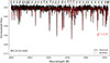 |
Fig. 3. Observed normalised spectrum (black solid line) of PG1514+034 and the best-fitting GSSP model to the cool companion lines (red dotted) for the wavelength range of 6000–6260 Å, used to determine the stellar atmospheric parameters of the cool companion. |
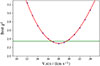 |
Fig. 4. The process of obtaining v sin i and its error interval for the cool companion of PG1514+034. The fitting of the polynomial function (in red) to the reduced χ2 coefficients (dark blue points) yields the outcome of the atmospheric parameter as the minimum, while the 1σ cut-off (green bar) provides its error interval. |
5. Observed properties
5.1. Galactic orbits and kinematics
The Galactic orbits of the wide hot subdwarf binaries were derived using such parameters as their coordinates (RA, Dec), distance, proper motions in the RA (pmra) and Dec (pmdec) directions, and systemic RV (γ). As an example, the Fig. 5 illustrates the derived Galactic orbit of the PG1514+034 system, computed using the Python package for Galactic dynamics, GALPY8.
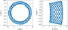 |
Fig. 5. Galactic orbit of PG1514+034 projected onto the Galactic plane (left) and the vertical Galactic component versus the radius with respect to the Galactic centre (right). |
The diagram in Fig. 6 shows the z-component of the angular momentum (JZ) against the eccentricity of the Galactic orbits for a calibration sample used by Pauli et al. (2006). The sample of wide hot sdB binaries has been incorporated into this diagram. The calibration sample consists of 291 F- and G-type MS stars, whose Galactic component memberships were previously determined based on both kinematic and chemical criteria (Edvardsson et al. 1993; Fuhrmann 1998, 2004). Three distinct regions (A, B, and C) can be identified in the diagram, predominantly populated by thin-disk, thick-disk, and halo stars, respectively. The positions of the wide sdB binary systems within the diagram suggest their probable Galactic population membership. However, the wide sdB binary sample consists of systems in which at least one companion has undergone post-MS evolution. Hence, it is an older and more metal-poor population, which could also be associated with more eccentric Galactic orbits and dynamically hotter kinematics (Wu et al. 2021; Nogueras-Lara et al. 2024).
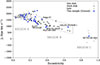 |
Fig. 6. JZ versus Galactic orbit eccentricity for the calibration sample of MS stars from Pauli et al. (2006). Region A is populated by thin disk stars, region B by thick disk stars, and region C by halo stars. The plot has been adapted to include the Galactic orbit parameters of the wide hot subdwarf sample. The wide sdB systems of the sample, which likely belong to the thick disk or the halo, are labelled. Error bars are included. |
The eccentricity and JZ of MCT0146-2651 (also known as SB744) strongly suggest its affiliation with the halo population. Following a recent study by Németh et al. (2021), the chemical analysis revealed a low metallicity ([M/H] = –1.09 dex), providing additional support (along with their kinematic parameters) for its likely halo membership.
For the Galactic kinematic study, the velocity components (U, V, W) of the sdB sample were determined using the criteria and calculations outlined in Johnson & Soderblom (1987). These velocities were corrected for solar motion relative to the local standard of rest (LSR) following the criteria of Coşkunoǧlu et al. (2011). The results are presented in a Toomre diagram in Fig. 7.
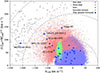 |
Fig. 7. Toomre diagram of the calibration sample by Chen et al. (2021) for the different Galactic components, attending to kinematics and stellar age criteria (see their paper for thresholds info). The calibration sample contains MS turn-off and subgiants stars from the solar neighbourhood to ≈1500 pc. The diagram has been adapted (in dimmed colours) to overlap the wide hot subdwarf binary sample. The sdB systems, which are more likely to belong to the thick disk or the halo, are labelled. Included error bars. |
The diagram includes a calibration sample from Chen et al. (2021) for the different Galactic components, incorporating data from the LAMOST MSTO-SG and Gaia DR2 catalogues. The classification of stars into various Galactic components was determined based on kinematic, chemical, and evolutionary considerations, as described in their study. Nevertheless, as generally accepted and indicated, stars with Vtot = (ULSR2 + VLSR2 + WLSR2)1/2 < 50 km s−1 predominantly, but not exclusively, belong to the thin disk, while those with moderate velocities Vtot ≈ 70 − 180 km s−1, are more typically associated with the thick disk (see e.g. Adibekyan et al. 2013; Bensby et al. 2014). Stars linked to the Hercules stream typically meet the criteria of VLSR ≈ −50 ± 9 km s−1 and (ULSR2 + WLSR2)1/2 ≈ 50 − 70 km s−1 (e.g. Famaey et al. 2005; Bensby et al. 2007). Finally, halo stars are typically characterised by Vtot > 220 km s−1 (Bonaca et al. 2017).
Most sdB systems are associated with the thin disk. However, consistent with Fig. 6, some systems are identified as probable candidates for the old thin disk or thick disk: BPS CS 22937, PG2148+095, Feige 87, EC 22540-3324, and JL277. GALEX J053939.1-283329 is a strong candidate for the thick disk, and MCT0146-2651 is identified as a halo system, in agreement with previous findings involving their Galactic orbits.
5.2. Parameter relations and comparison with binary evolution models
The determination of the complete set of orbital and cool companion atmospheric parameters for the current sample of wide hot sdB binaries represents an effort that spanned more than a decade of observations. Work is still underway to increase the number of systems. Nevertheless, the sample obtained so far enabled us to establish relationships between orbital and atmospheric parameters and to provide strong constraints on current theoretical frameworks.
The most detailed long-period sdB population study to date was carried out by Vos et al. (2020), using a combination of detailed stellar evolution simulations based on Modules for Experiments in Stellar Astrophysics (MESA; Paxton et al. 2011, 2013, 2015, 2018, 2019), the observationally calibrated Besançon Galactic population model (Robin et al. 2003), a model for synthetic observations, and a standard model of binary interactions.
In Fig. 8, we show the CMD from Fig. 1, but this time including simulations from Vos et al. (2020). We note that a significant number of spectroscopic wide sdB binaries occupy a region predicted by the Vos et al. (2020) theoretical model to contain SB1 systems and they are thus offset from the predictions for composite sdB simulations (left panel).
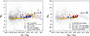 |
Fig. 8. Same CMD diagram than in Fig. 1 but including the simulations by Vos et al. (2020). Left: Brown filled circles indicating sdB SB1 observable simulations and yellow filled ones for observable sdB composites, according to the visibility criteria of the theoretical work. Right: Only including simulations of observable sdB composites as yellow filled circles. The systems in the wide sdB sample with cool companions whose Teff is higher than 6000 K are marked with red filled circles. |
The study of the RV curves provides insight into the orbital period distribution of the wide hot sdB sample. The orbital period distribution has been studied since the theoretical work by Vos et al. (2020). Figure 9 shows the histogram of predicted orbital period distributions from the simulations, based on the visibility criteria, in agreement with the Galactic model.
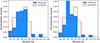 |
Fig. 9. Distribution histogram of orbital periods and the predicted period distributions from the MESA simulations, according to the Galactic model by Vos et al. (2020). Left: Distribution histogram of the wide sdB binary systems sample not including Gaia wide sdB candidates. Right: Distribution histogram including both, the wide sdB binary systems sample and Gaia wide sdB candidates. |
To construct this histogram, the same method used by Vos et al. (2013) was employed, treating each observation as a normal distribution with the error as the standard deviation. Subsequently, 1000 orbital periods per system were randomly generated within the uncertainty interval. The resulting 32 000 points (from 32 systems) were binned into intervals of 200 days. The inclusion of wide sdB Gaia-based candidates in the orbital period distribution is notably disruptive in the comparison between theoretical and observational distributions.
The eccentricity of observed binary systems has long challenged theoretical models. Tidal forces are typically expected to lead to orbital circularisation. However, observations suggest that eccentricity appears to increase with longer orbital periods (see Fig. 10A).
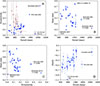 |
Fig. 10. Correlations between orbital parameters derived from the RV curves of the wide sdB binary systems. The ground-based sample is shown as blue filled circles. Meanwhile, the Gaia-based sample is depicted as red empty diamonds when data is available (Panel A). Error bars are included. Panel A: Diagram of the orbital period-eccentricity correlation. Panel B: Diagram of the orbital period-mass ratio correlation. Panel C: Diagram of the eccentricity-mass ratio correlation. Panel D: Diagram of the orbital period-metallicity correlation. |
Vos et al. (2015) proposed a theoretical framework to explain this feature, based on the combination of two eccentricity-pumping mechanisms: a phase-dependent RLOF and the formation of a circumbinary disk (CB), which can increase the final eccentricities of the systems. However, while the model successfully accounts for most systems, it is not a population model and does not fully reproduce the observed distribution of systems with the longest and shortest orbital periods. Figure 11 illustrates the agreement between the observations and the theoretical regions predicted by the eccentricity mechanisms from Vos et al. (2015). The Gaia-based candidate sample further reinforces the apparent discrepancy with the wide sdB sample obtained through spectroscopic methods, but in addition to theoretical models. This might indicate another part of the population detected by Gaia using astrometric methods. However, their large uncertainties prevented us from determining any strong conclusions in this regard.
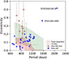 |
Fig. 11. Adapted diagram of the orbital period-eccentricity correlation from Vos et al. (2015, see Fig. 9). The red-shaded area represents the region explained by RLOF models, while the green-shaded area corresponds to a model incorporating a CB disk formation. The ground-based sample is shown as blue filled circles and the Gaia-based one as red empty diamonds. Error bars are included. |
The correlation between orbital period and mass ratio (P − q) in wide sdB binaries was addressed by Vos et al. (2020). Their population study concluded that this correlation is strongly linked to the metallicity history of the Galaxy. Furthermore, the model predicts the final P − q relation in the context of the Galactic membership of the systems. Figure 10B shows the P − q observations. In Fig. 12 they are compared to the model of Vos et al. (2020, see their Fig. 7). The sdB systems are colour-coded based on their probable membership in the Galactic population, which we define using Galactic orbit eccentricity and the boundaries from the calibrated sample by Pauli et al. (2006) in Fig. 6, as well as the kinematic regions in Fig. 7. Systems with a Galactic orbital eccentricity lower than 0.15 were classified as strong Galactic thin disk candidates. Systems with Galactic orbital eccentricities between 0.15 and 0.45 were classified as a mixture of old thin disk and thick disk (i.e. belonging to either Region A or B). The system GALEX J053939.1-283329 in Region B, with an eccentricity higher than 0.45, consistent with its kinematics, was identified as a strong thick disk candidate. Finally, the system in Region C, MCT0146-2651 is defined as a strong halo candidate, given its high Galactic orbital eccentricity and low Jz, as well as its kinematics and low metallicity.
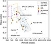 |
Fig. 12. Adapted diagram of the orbital period-mass ratio correlation from Vos et al. (see Fig. 7; 2020). Simulations of wide sdB are shown as sky-filled squares. The regions where wide sdBs formed from different Galactic subpopulations are expected to be located are colour-coded: thin-disk objects in gray, thick-disk objects in orange, and halo objects in purple. Similarly, the observed systems are colour-coded according to their likely Galactic membership. Systems with an unclear Galactic membership to either the thin or thick disk due to the old population of wide sdB binaries are labelled into the single category old thin/thick. See Sects. 5.1 and 5.2 for a further explanation. |
The binary model by Vos et al. (2020) also predicts a theoretical relationship between the final orbital periods and the metallicity of the systems. Figure 10D shows the parameters derived from the observations, which are compared with the region predicted by the model. The general agreement is reasonably good. Some outliers are observed, including the two systems with the longest orbital periods (notably, by approximately a factor of two compared to the rest), EC03563-3618 and PG2148+095, as was also the case in the P − Ecc correlation. MCT0146-2651 (or SB744), likely a halo member based on its Galactic orbit parameters, kinematics, and metallicity, might also be potentially deviating from the overall relation.
6. Discussion
The parameter results obtained from the wide sdB sample were compared with current theoretical models in the previous section. Interesting insights emerge from both the agreements and the discrepancies observed.
6.1. Colour-magnitude diagram
In the CMD (see Fig. 8) the simulated composite sdB systems exhibit BP − RP colours bluer than 0.3 and are dimmer by up to ≈1 G-band magnitude than the spectroscopic wide sdB sample. Indeed, a similar conclusion can be drawn for the majority of the composite sdB sample, as reported by Pelisoli et al. (2020), which is included in the CMD.
A close analysis of the wide sdB systems showing colours beyond 0.3, apart from the SG system BD-07 5977 (Vos et al. 2017), indicates that they correspond mostly to those sdB containing cool companions with Teff higher than 6000 K (see the right panel of Fig. 8). Hence, stars are likely to belong to the F- or earliest G-type spectral class at least. This is indicative that the Vos et al. (2020) model is overpredicting the number of the sdBs with the coolest companions. Observational data from the wide sdB sample will likely help improve the visibility criteria in ongoing and future theoretical works.
6.2. Orbital period distribution
The Gaia-based sample consistently exhibits discrepant behaviour across the different comparisons with respect to the ground-based spectroscopic sample. This is also evident in the orbital period distribution shown in Fig. 9 (right panel), when their P values are included. The discrepancy could arise from an observational bias affecting the Gaia sample, since the selection criteria for the Gaia binaries are not identical to those used for the spectroscopic sample. The reported orbital periods tend to cluster in the 700–900-day range, with significant uncertainties in some systems. Alternatively, these Gaia candidates might indicate the existence of a new population of wide sdB systems that has not yet been accounted for by the spectroscopically confirmed sample. Their positions in the above-mentioned CMD diagrams indicate fainter absolute magnitudes than populations of the current wide sdB or Pelisoli’s composite samples.
Whether this discrepancy arises from a selection effect favouring a subset of wide sdB systems has been explored in the recent work of Nagarajan et al. (2026). The authors argued that Gaia DR3 is preferentially sensitive to systems with orbital periods below or about 1000 d and relatively large photocentre semi-major axes (ao). They further showed that the detectability of the photocentre motion depends strongly on the flux ratio and the companion properties, as well as the orbital geometry. They also showed that spectroscopic systems tend to have low Gaia detection probabilities. In contrast, astrometric detected systems are preferentially located in the region where Gaia’s photocentre sensitivity is highest.
Therefore, directly comparing the two observed samples without accounting for their respective selection functions can lead to apparent disagreements that are observational rather than physical. As a result, the Gaia astrometric sample is expected to represent a biased subset of the sdB population, concentrated in the period range where DR3 orbital solutions are most efficient, namely clustered between 600 and 1000 d.
This readily explains why the Gaia-based candidates appear to differ from the ground-based spectroscopic sample in their period distribution. The same argument may also apply to eccentricity: Gaia eccentricities are derived from astrometric photocentre-orbit solutions and often carry significant uncertainties, so part of the apparent discrepancy in the period-eccentricity diagram may reflect measurement systematics and selection effects rather than a true astrophysical difference (see Figs. 10A and 11A).
The CMD behaviour is also consistent with this interpretation, according to the cited authors. The different location of the Gaia candidates in the CMD diagram reflects differences in companion properties and flux ratios, which, in turn, affect Gaia astrometric detectability. Ground-based spectroscopic studies typically require systems with measurable RVs and identifiable spectral contributions from one or both components, whereas Gaia astrometric solutions favour systems with measurable photocentre motion.
6.3. The eccentricity question
As highlighted in Sect. 5.2, the eccentricity of wide sdB systems has long challenged theoretical models because the first systems observed showed unexpectedly high eccentricities at longer orbital periods. Nevertheless, a closer look at Fig. 10A leads us to conclude that when excluding the two systems with unexpectedly long periods (and the largest eccentricities), the remaining systems do not exhibit such a strong correlation, as initially indicated by the first solved systems more than a decade ago. In our view, this suggests that additional complex factors might be involved in defining the final eccentricity of the systems.
Similarly to the orbital period distribution, the incorporation of the wide sdB Gaia candidates is disruptive in the diagram. This inconsistency may reflect an observational bias between the Gaia and spectroscopic samples, as previously noted regarding the CMD diagram and the orbital period issues. Nonetheless, it should be observed that the Gaia eccentricity measurements are subject to large uncertainties. On the other hand, a similar discrepancy between the eccentricity obtained by Gaia and the ground-based RV measurements of the binary system BD+20 5391 has been observed by Kurpas et al. (2025). The authors concluded that Gaia was likely overestimating the eccentricity of the binary system.
As outlined in Sect. 5.2, the theoretical framework proposed by Vos et al. (2015) to address the unresolved eccentricity problem is based on the formation of a CB disk during the mass-loss phase. However, empirical evidence has not yet supported this scenario.
However, this idea is further reinforced by the numerous detections and evidence of dusty disks around binary systems, such as eccentric post-AGB binaries (see e.g. Kluska et al. 2022; Oomen et al. 2020, 2018; van Winckel 2017), post-RGB systems (Sarkar & Sahai 2022b; Kamath 2015; Montgomery & Welsh 2012), and post-common-envelope (post-CE) binaries such as the WD binary NN Serpentis (Hardy et al. 2016) or the recently published one involving a sample of post-CE close hot subdwarf binaries (Li et al. 2025).
The formation of dust and the associated dusty and debris discs in binary systems has also been addressed from the theoretical point of view (see e.g. Bermúdez-Bustamante et al. 2024; González-Bolívar et al. 2024; Sarkar & Sahai 2022a; Thebault et al. 2021). Although the gas would be removed early on from a potential CB disk in wide sdB binaries due to photoevaporation, this mechanism is argued to be inefficient for the destruction of relatively small grains (≥0.01 μm), even in the presence of a strong radiation field (Nanni et al. 2024). Hence, dust grains could have survived the He core and shell-burning phase. Partially supporting this idea, the recent work by Li et al. (2025) argues for the indirect detection of long-lived circumstellar material around close hot subdwarf binaries as likely remnants of their past CE phase. If remnant material from past CB discs is still linked to wide sdB binaries, contrary to the optically thick discs of Post-AGB or -RGB, a negligible excess in near-IR should be expected (see e.g. transition disks detected in Post-AGB by Kluska et al. 2022).
Two systems from the wide sdB sample show a slight IR excess in the Longwave-IR WISE W4 band, BD-11 162 and BD-7 5977. They were studied with the ALMA radio telescope (Molina et al. 2022). However, no remnants of a CB disk were detected. In the case of BD-7 5977, the IR excess may be attributed to the subgiant nature of the cool companion (Vos et al. 2017). Nevertheless, these results do not rule out the presence of a CB disk in the history of these systems.
According to the previously outlined arguments, the direct detection is complicated, and indirect mechanisms should be developed, as utilised by Li et al. (2025). Their analysis was based on the presence of the Ca II K line, which is linked to the system. This line has been widely used in various studies to trace both transient and stable absorption features from CSM and dusty disks around different types of systems (see e.g. Vanderbosch et al. 2020; Rebollido et al. 2018; Iglesias et al. 2018; Welsh & Montgomery 2016; Montgomery & Welsh 2012). However, this work was recently revisited in the master’s thesis of Weich (2025). That analysis raises doubts about the conclusions of Li et al. (2025), as the reported CSM signatures may be affected by methodological limitations, particularly with respect to uncertainties in the reddening estimates, the use of a Ca II EW–reddening comparison that is not universally applicable, the reliance on low-resolution spectra, and the contamination of the sample by composite sdB systems. Taken together, these issues considerably weaken the evidence for CSM in the Li et al. (2025) sample.
6.4. Mass ratio and orbital period relation
The work of Vos et al. (2020) demonstrated that the P − q distribution of the wide sdBs is partly determined by the metallicity history of the Galaxy and was able to reproduce the observed formation rates, metallicity, period, and mass-ratio distributions. Comparing the P − q relation for the observed ground-based sample, classified by its Galactic membership, with the simulated sample from Vos et al. (2020) in Fig. 12, we find both good agreement and new open questions.
We can see that the bulk of the thin disk lies in the main part of the P − q relation, overlapping with the simulated sample. The systems with a low mass ratio (< 0.35) and shorter orbital periods (< 1000 d), PB6355 and HE0430-2457, are consistent with being the extension of the Vos et al. (2020) population towards younger and more massive, non-degenerately igniting progenitors. The halo candidate system MCT0146-2651 is consistent with the metal-rich end of the Galactic halo, noting that the Besançon model used in Vos et al. (2020) assumes an overly narrow metallicity range for the halo. The strong thick disk candidate GALEX J053939.1 is consistent with the metal-rich part of the Galactic thick disk. Finally, the region with mass ratios of 0.5–0.6 and periods below 750 d, considered to be an unexplained second branch in Vos et al. (2020), can now be seen to mostly consist of old stars, offering a strong clue to its explanation in the population model. EC03563-3618, along with PG 2148+095, stands out for having an orbital period that is very hard to explain solely using binary models. Both systems may be products of triple stellar evolution (Toonen et al. 2016; Preece et al. 2022; Shariat et al. 2025). Finally, the clustering of binaries in several regions of the P − q plane, as well as an excess of systems with P close to 1250 d are new emerging features that require further explanation.
6.5. Metallicity evolution
The metallicity of the wide sdB sample is reasonably well reproduced by the simulations of Vos et al. (2020) shown in Fig. 13, except for the three outlier systems highlighted in Sect. 5.2. The outlier MCT0146-2651, is the only halo disc candidate of the sample. Its sdB companion exhibits heavy-metal signatures (such as lead and fluorine), which led Németh et al. (2021) to conclude that its formation probably resulted from a merger event in a hierarchical triple system. However, given that the system belongs to the binary population, the most likely explanation is that the heavy-metal signatures result from initial abundances and binary evolution. Interestingly, EC03563-3618, another outlier given its long P, exhibits spectral disturbances that suggest the presence of an additional companion or circumstellar material; possibly an unseen, very long-period cool dwarf. This matter requires further research to confirm or refute.
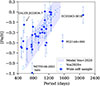 |
Fig. 13. Orbital period versus metallicity for wide sdB binaries. The pale blue region represents the theoretical correlation predicted by Vos et al. (2020), based on a Galactic evolution model combined with a deterministic binary interaction model. Simulations of wide sdB are shown as sky-filled squares, wide sdB binaries sample as blue filled circles. Error bars are included. |
At the same time, the second-branch systems in Vos et al. (2020), with orbital periods below 750 d belong to the continuation of the same trend in Fig. 13, again suggesting that they are part of the same population.
7. Conclusions
We obtained the orbital parameters of the 32 wide sdB binary systems. The data come from high-resolution spectra gathered over more than a decade and a half.
Excluding the two outlier systems, EC03563-3618 and PG2148+095, the orbital period distribution of the ground-based wide sdB sample shows a good agreement with the Galactic population synthesis model of Vos et al. (2020). The differences become more pronounced when the Gaia-wide sdB sample is included.
The Gaia sample shows an anti-correlation between orbital period and eccentricity. However, two factors prevent us from drawing further conclusions: the large uncertainties in the Gaia eccentricity measurements and the narrow orbital period range (700–900 days) where most systems are located. A recent study which investigated Gaia’s selection function, supports the interpretation that the correlation observed in the Gaia-based sample is driven by selection effects and, in part, by measurement systematics.
Notably, no cross-matching records were obtained from the NSS files for sources compatible with a double-lined spectroscopic binary (SB2) model, even though the NSS files contain more than 5000 records. This may be significant for the orbital parameters and features of the Gaia sample. Several of the Gaia systems are currently being monitored. Gaia parameters and those derived from comparisons with high-resolution spectroscopy will help clarify this issue.
In contrast, the ground-based sample of wide sdB systems, excluding the two aforementioned outliers, does not show a clear linear relationship between orbital period and eccentricity. This stands in contrast to earlier studies that suggested otherwise and were based on a smaller number of systems.
In a forthcoming work, the mass distributions of the companions in these systems will be derived using a method that combines spectroscopic, photometric, and evolutionary model approaches. The availability of absolute masses will provide other valuable parameters, including absolute separations and orbital inclinations. It will enable further analyses of the rotation periods of the companions and help identify entirely new parameter correlations, providing further strong constraints on binary evolution. We hope that this comprehensive set of wide sdB binaries will contribute to a better understanding of their formation and their main evolutionary properties.
Data availability
Tables A.1, B.1, B.2, and B.3 are available at the CDS via https://cdsarc.cds.unistra.fr/viz-bin/cat/J/A+A/710/A280
Acknowledgments
J.V. acknowledges support from the Grant Agency of the Czech Republic (GAČR 22-34467S). M.V. acknowledges funding support from the Fondecyt Regular projects 1211491 and 1250525. A.B. acknowledges support from the Australian Research Council (ARC) Centre of Excellence for Gravitational Wave Discovery (OzGrav), through project number CE230100016. This work has made use of data from the European Space Agency (ESA) mission Gaia (https://www.cosmos.esa.int/gaia), processed by the Gaia Data Processing and Analysis Consortium (DPAC, https://www.cosmos.esa.int/web/gaia/dpac/consortium). Funding for the DPAC has been provided by national institutions, in particular the institutions participating in the Gaia Multilateral Agreement. Based on observations collected at the European Southern Observatory under ESO programs 088.D-0364, 093.D-0629, 096.D-0180, 097.D-0110, 098.D-0018, 099.D-0014, 0100.D-0082, 0101.D-0200, 0102.D-0255, 0103.D-0129, 0104.D-0135, 105.20L2.001, 106.2105.001, 113.26RL.001, 114.274R.001, 115.287Y.001 and 116.28ZZ.001.
References
- Adibekyan, V. Z., Figueira, P., Santos, N. C., et al. 2013, A&A, 554, A44 [NASA ADS] [CrossRef] [EDP Sciences] [Google Scholar]
- Arancibia-Rojas, E., Zorotovic, M., Vučković, M., et al. 2024, MNRAS, 527, 11184 [Google Scholar]
- Bensby, T., Zenn, A. R., Oey, M. S., & Feltzing, S. 2007, ApJ, 663, L13 [CrossRef] [Google Scholar]
- Bensby, T., Feltzing, S., & Oey, M. S. 2014, A&A, 562, A71 [NASA ADS] [CrossRef] [EDP Sciences] [Google Scholar]
- Bermúdez-Bustamante, L. C., De Marco, O., Siess, L., et al. 2024, MNRAS, 533, 464 [Google Scholar]
- Binnendijk, L. 1960, Properties of Double Stars; A Survey of Parallaxes and Orbits (University of Pennsylvania Press) [Google Scholar]
- Bohlin, R. C., Mészáros, S., Fleming, S. W., et al. 2017, AJ, 153, 234 [Google Scholar]
- Bonaca, A., Conroy, C., Wetzel, A., Hopkins, P. F., & Kereš, D. 2017, ApJ, 845, 101 [NASA ADS] [CrossRef] [Google Scholar]
- Brassard, P., Fontaine, G., Billères, M., et al. 2001, ApJ, 563, 1013 [CrossRef] [Google Scholar]
- Bruntt, H., Bedding, T. R., Quirion, P. O., et al. 2010, MNRAS, 405, 1907 [Google Scholar]
- Chen, X., Han, Z., Deca, J., & Podsiadlowski, P. 2013, MNRAS, 434, 186 [Google Scholar]
- Chen, D.-C., Xie, J.-W., Zhou, J.-L., et al. 2021, ApJ, 909, 115 [NASA ADS] [CrossRef] [Google Scholar]
- Coşkunoǧlu, B., Ak, S., Bilir, S., et al. 2011, MNRAS, 412, 1237 [NASA ADS] [Google Scholar]
- Culpan, R., Geier, S., Reindl, N., et al. 2022, A&A, 662, A40 [NASA ADS] [CrossRef] [EDP Sciences] [Google Scholar]
- Deca, J., Marsh, T. R., Østensen, R. H., et al. 2012, MNRAS, 421, 2798 [Google Scholar]
- Downes, R. A. 1986, ApJS, 61, 569 [NASA ADS] [CrossRef] [Google Scholar]
- Doyle, A. P., Davies, G. R., Smalley, B., Chaplin, W. J., & Elsworth, Y. 2014, MNRAS, 444, 3592 [Google Scholar]
- Edvardsson, B., Andersen, J., Gustafsson, B., et al. 1993, A&A, 275, 101 [NASA ADS] [Google Scholar]
- Famaey, B., Jorissen, A., Luri, X., et al. 2005, A&A, 430, 165 [CrossRef] [EDP Sciences] [Google Scholar]
- Fuhrmann, K. 1998, A&A, 338, 161 [NASA ADS] [Google Scholar]
- Fuhrmann, K. 2004, Astron. Nachr., 325, 3 [NASA ADS] [CrossRef] [Google Scholar]
- Gaia Collaboration (Arenou, F., et al.) 2023a, A&A, 674, A34 [CrossRef] [EDP Sciences] [Google Scholar]
- Gaia Collaboration (Vallenari, A., et al.) 2023b, A&A, 674, A1 [NASA ADS] [CrossRef] [EDP Sciences] [Google Scholar]
- Geier, S. 2020, A&A, 635, A193 [NASA ADS] [CrossRef] [EDP Sciences] [Google Scholar]
- Geier, S., Østensen, R. H., Nemeth, P., et al. 2017, A&A, 600, A50 [NASA ADS] [CrossRef] [EDP Sciences] [Google Scholar]
- González-Bolívar, M., De Marco, O., Bermúdez-Bustamante, L. C., Siess, L., & Price, D. J. 2024, MNRAS, 527, 9145 [Google Scholar]
- Gorlova, N., Van Winckel, H., Vos, J., et al. 2013, EAS Publ. Ser., 64, 163 [Google Scholar]
- Gosset, E., Damerdji, Y., Morel, T., et al. 2025, A&A, 693, A124 [NASA ADS] [CrossRef] [EDP Sciences] [Google Scholar]
- Green, R. F., Schmidt, M., & Liebert, J. 1986, ApJS, 61, 305 [NASA ADS] [CrossRef] [Google Scholar]
- Halbwachs, J.-L., Pourbaix, D., Arenou, F., et al. 2023, A&A, 674, A9 [NASA ADS] [CrossRef] [EDP Sciences] [Google Scholar]
- Han, Z., Tout, C. A., & Eggleton, P. P. 2000, MNRAS, 319, 215 [Google Scholar]
- Han, Z., Podsiadlowski, P., Maxted, P. F. L., Marsh, T. R., & Ivanova, N. 2002, MNRAS, 336, 449 [Google Scholar]
- Han, Z., Podsiadlowski, P., Maxted, P. F. L., & Marsh, T. R. 2003, MNRAS, 341, 669 [NASA ADS] [CrossRef] [Google Scholar]
- Hardy, A., Schreiber, M. R., Parsons, S. G., et al. 2016, MNRAS, 459, 4518 [NASA ADS] [CrossRef] [Google Scholar]
- Heber, U. 2009, ARA&A, 47, 211 [Google Scholar]
- Heber, U. 2016, PASP, 128, 082001 [Google Scholar]
- Hilditch, R. W. 2001, An Introduction to Close Binary Stars (Cambridge University Press) [Google Scholar]
- Hubeny, I., & Lanz, T. 2017, arXiv e-prints [arXiv:1706.01937] [Google Scholar]
- Iglesias, D., Bayo, A., Olofsson, J., et al. 2018, MNRAS, 480, 488 [Google Scholar]
- Johnson, D. R. H., & Soderblom, D. R. 1987, AJ, 93, 864 [Google Scholar]
- Kamath, D. 2015, EAS Publ. Ser., 71–72, 129 [Google Scholar]
- Kilkenny, D., Heber, U., & Drilling, J. S. 1988, South Afr. Astron. Obs. Circ., 12, 1 [NASA ADS] [Google Scholar]
- Kluska, J., Van Winckel, H., Coppée, Q., et al. 2022, A&A, 658, A36 [NASA ADS] [CrossRef] [EDP Sciences] [Google Scholar]
- Kurpas, M., Dorsch, M., Geier, S., et al. 2025, A&A, 702, A200 [NASA ADS] [CrossRef] [EDP Sciences] [Google Scholar]
- Kurucz, R. L. 1979, ApJS, 40, 1 [NASA ADS] [CrossRef] [Google Scholar]
- Li, J., Wolf, C., Li, J., et al. 2025, MNRAS, 537, 1950 [Google Scholar]
- Lindegren, L., Hernández, J., Bombrun, A., et al. 2018, A&A, 616, A2 [NASA ADS] [CrossRef] [EDP Sciences] [Google Scholar]
- Mengel, J. G., Norris, J., & Gross, P. G. 1975, BAAS, 7, 256 [NASA ADS] [Google Scholar]
- Molina, F., Vos, J., Németh, P., et al. 2022, A&A, 658, A122 [NASA ADS] [CrossRef] [EDP Sciences] [Google Scholar]
- Montgomery, S. L., & Welsh, B. Y. 2012, PASP, 124, 1042 [CrossRef] [Google Scholar]
- Nagarajan, P., El-Badry, K., Bobrick, A., et al. 2026, PASP, 138, 044205 [Google Scholar]
- Nanni, A., Cristallo, S., Donevski, D., et al. 2024, A&A, 684, A163 [NASA ADS] [CrossRef] [EDP Sciences] [Google Scholar]
- Nemeth, P. 2019, ASP Conf. Ser., 519, 117 [NASA ADS] [Google Scholar]
- Németh, P., Kawka, A., & Vennes, S. 2012, MNRAS, 427, 2180 [Google Scholar]
- Németh, P., Vos, J., Molina, F., & Bastian, A. 2021, A&A, 653, A3 [Google Scholar]
- Nogueras-Lara, F., Nieuwmunster, N., Schultheis, M., et al. 2024, A&A, 690, A313 [NASA ADS] [CrossRef] [EDP Sciences] [Google Scholar]
- Oomen, G.-M., Van Winckel, H., Pols, O., et al. 2018, A&A, 620, A85 [NASA ADS] [CrossRef] [EDP Sciences] [Google Scholar]
- Oomen, G.-M., Pols, O., Van Winckel, H., & Nelemans, G. 2020, A&A, 642, A234 [NASA ADS] [CrossRef] [EDP Sciences] [Google Scholar]
- Østensen, R. H. 2006, Balt. Astron., 15, 85 [NASA ADS] [Google Scholar]
- Østensen, R. H., & Van Winckel, H. 2012, ASP Conf. Ser., 452, 163 [Google Scholar]
- Paczynski, B. 1976, IAU Symp., 73, 75 [NASA ADS] [Google Scholar]
- Pauli, E. M., Napiwotzki, R., Heber, U., Altmann, M., & Odenkirchen, M. 2006, A&A, 447, 173 [NASA ADS] [CrossRef] [EDP Sciences] [Google Scholar]
- Paxton, B., Bildsten, L., Dotter, A., et al. 2011, ApJS, 192, 3 [Google Scholar]
- Paxton, B., Cantiello, M., Arras, P., et al. 2013, ApJS, 208, 4 [Google Scholar]
- Paxton, B., Marchant, P., Schwab, J., et al. 2015, ApJS, 220, 15 [Google Scholar]
- Paxton, B., Schwab, J., Bauer, E. B., et al. 2018, ApJS, 234, 34 [NASA ADS] [CrossRef] [Google Scholar]
- Paxton, B., Smolec, R., Schwab, J., et al. 2019, ApJS, 243, 10 [Google Scholar]
- Pelisoli, I., Vos, J., Geier, S., Schaffenroth, V., & Baran, A. S. 2020, A&A, 642, A180 [NASA ADS] [CrossRef] [EDP Sciences] [Google Scholar]
- Preece, H. P., Hamers, A. S., Battich, T., & Rajamuthukumar, A. S. 2022, MNRAS, 517, 2111 [NASA ADS] [CrossRef] [Google Scholar]
- Raskin, G., van Winckel, H., Hensberge, H., et al. 2011, A&A, 526, A69 [CrossRef] [EDP Sciences] [Google Scholar]
- Rebollido, I., Eiroa, C., Montesinos, B., et al. 2018, A&A, 614, A3 [NASA ADS] [CrossRef] [EDP Sciences] [Google Scholar]
- Rhee, J., Seibert, M., Østensen, R. H., et al. 2006, Balt. Astron., 15, 77 [NASA ADS] [Google Scholar]
- Robin, A. C., Reylé, C., Derrière, S., & Picaud, S. 2003, A&A, 409, 523 [NASA ADS] [CrossRef] [EDP Sciences] [Google Scholar]
- Saffer, R. A., Bergeron, P., Koester, D., & Liebert, J. 1994, ApJ, 432, 351 [NASA ADS] [CrossRef] [Google Scholar]
- Sarkar, G., & Sahai, R. 2022a, ApJ, 940, 54 [Google Scholar]
- Sarkar, G., & Sahai, R. 2022b, IAU Symp., 366, 314 [Google Scholar]
- Shariat, C., El-Badry, K., & Naoz, S. 2025, PASP, 137, 094201 [Google Scholar]
- Shulyak, D., Tsymbal, V., Ryabchikova, T., Stütz, C., & Weiss, W. W. 2004, A&A, 428, 993 [NASA ADS] [CrossRef] [EDP Sciences] [Google Scholar]
- Simon, K. P., & Sturm, E. 1994, A&A, 281, 286 [NASA ADS] [Google Scholar]
- Stark, M. A., & Wade, R. A. 2003, AJ, 126, 1455 [NASA ADS] [CrossRef] [Google Scholar]
- Taylor, M. B. 2005, ASP Conf. Ser., 347, 29 [Google Scholar]
- Thebault, P., Kral, Q., & Olofsson, J. 2021, A&A, 646, A173 [NASA ADS] [CrossRef] [EDP Sciences] [Google Scholar]
- Tkachenko, A. 2015, A&A, 581, A129 [NASA ADS] [CrossRef] [EDP Sciences] [Google Scholar]
- Toonen, S., Hamers, A., & Portegies Zwart, S. 2016, Comput. Astrophys. Cosmol., 3, 6 [NASA ADS] [CrossRef] [Google Scholar]
- Tsymbal, V. 1996, ASP Conf. Ser., 108, 198 [Google Scholar]
- van Winckel, H. 2017, IAU Symp., 323, 231 [NASA ADS] [Google Scholar]
- Vanderbosch, Z., Hermes, J. J., Dennihy, E., et al. 2020, ApJ, 897, 171 [Google Scholar]
- Vos, J., Østensen, R. H., Degroote, P., et al. 2012, A&A, 548, A6 [NASA ADS] [CrossRef] [EDP Sciences] [Google Scholar]
- Vos, J., Østensen, R. H., Németh, P., et al. 2013, A&A, 559, A54 [NASA ADS] [CrossRef] [EDP Sciences] [Google Scholar]
- Vos, J., Østensen, R. H., Marchant, P., & Van Winckel, H. 2015, A&A, 579, A49 [NASA ADS] [CrossRef] [EDP Sciences] [Google Scholar]
- Vos, J., Østensen, R. H., Vučković, M., & Van Winckel, H. 2017, A&A, 605, A109 [NASA ADS] [CrossRef] [EDP Sciences] [Google Scholar]
- Vos, J., Németh, P., Vučković, M., Østensen, R., & Parsons, S. 2018, MNRAS, 473, 693 [NASA ADS] [CrossRef] [Google Scholar]
- Vos, J., Vučković, M., Chen, X., et al. 2019, MNRAS, 482, 4592 [NASA ADS] [CrossRef] [Google Scholar]
- Vos, J., Bobrick, A., & Vučković, M. 2020, A&A, 641, A163 [NASA ADS] [CrossRef] [EDP Sciences] [Google Scholar]
- Wade, R. A., Stark, M. A., Green, R. F., & Durrell, P. R. 2006, Balt. Astron., 15, 81 [Google Scholar]
- Webbink, R. F. 1984, ApJ, 277, 355 [NASA ADS] [CrossRef] [Google Scholar]
- Weich, S. 2025, Master’s Thesis, Friedrich-Alexander-Universität Erlangen-Nürnberg [Google Scholar]
- Welsh, B. Y., & Montgomery, S. 2016, PASP, 128, 064201 [NASA ADS] [CrossRef] [Google Scholar]
- Wu, Y., Xiang, M., Chen, Y., et al. 2021, MNRAS, 501, 4917 [NASA ADS] [CrossRef] [Google Scholar]
All Tables
All Figures
|
Fig. 1. Left: CMD presented by Pelisoli et al. (2020) for their composite hot subdwarf sample is shown as dimmed red diamonds, representing systems whose light curves and rotation periods were studied by the authors. We included the wide hot sdB binary ground-based sample with fully solved orbital parameters as blue filled circles. The Gaia-based sample is shown as green empty diamonds. Interstellar extinctions for both, ground- and Gaia-based samples, are not corrected. Stars catalogued by Geier (2020) as hot subdwarfs are represented as dark gray open circles. MS stars and stars in other evolutionary stages within the region by Lindegren et al. (sample C; 2018) are shown as pale gray dots. Right: Aitoff projection displaying the Galactic coordinates of the wide hot sdB sample. Galactic longitude increases from the centre toward the left, with increments of 30° per tick. Same colour-coded wide sdB systems are shown. |
| In the text | |
|
Fig. 2. RV curves and residuals for PG1514+034. The RVs of the cool companion are plotted as green filled circles, while those of the sdB companion are shown as blue filled squares. RV error bars (1σ), obtained through MC simulations, are included. The best-fit Keplerian orbits, simultaneously fitted for both the MS and sdB companions, are represented by a solid line for the cool companion and a dotted line for the hot one. |
| In the text | |
|
Fig. 3. Observed normalised spectrum (black solid line) of PG1514+034 and the best-fitting GSSP model to the cool companion lines (red dotted) for the wavelength range of 6000–6260 Å, used to determine the stellar atmospheric parameters of the cool companion. |
| In the text | |
|
Fig. 4. The process of obtaining v sin i and its error interval for the cool companion of PG1514+034. The fitting of the polynomial function (in red) to the reduced χ2 coefficients (dark blue points) yields the outcome of the atmospheric parameter as the minimum, while the 1σ cut-off (green bar) provides its error interval. |
| In the text | |
|
Fig. 5. Galactic orbit of PG1514+034 projected onto the Galactic plane (left) and the vertical Galactic component versus the radius with respect to the Galactic centre (right). |
| In the text | |
|
Fig. 6. JZ versus Galactic orbit eccentricity for the calibration sample of MS stars from Pauli et al. (2006). Region A is populated by thin disk stars, region B by thick disk stars, and region C by halo stars. The plot has been adapted to include the Galactic orbit parameters of the wide hot subdwarf sample. The wide sdB systems of the sample, which likely belong to the thick disk or the halo, are labelled. Error bars are included. |
| In the text | |
|
Fig. 7. Toomre diagram of the calibration sample by Chen et al. (2021) for the different Galactic components, attending to kinematics and stellar age criteria (see their paper for thresholds info). The calibration sample contains MS turn-off and subgiants stars from the solar neighbourhood to ≈1500 pc. The diagram has been adapted (in dimmed colours) to overlap the wide hot subdwarf binary sample. The sdB systems, which are more likely to belong to the thick disk or the halo, are labelled. Included error bars. |
| In the text | |
|
Fig. 8. Same CMD diagram than in Fig. 1 but including the simulations by Vos et al. (2020). Left: Brown filled circles indicating sdB SB1 observable simulations and yellow filled ones for observable sdB composites, according to the visibility criteria of the theoretical work. Right: Only including simulations of observable sdB composites as yellow filled circles. The systems in the wide sdB sample with cool companions whose Teff is higher than 6000 K are marked with red filled circles. |
| In the text | |
|
Fig. 9. Distribution histogram of orbital periods and the predicted period distributions from the MESA simulations, according to the Galactic model by Vos et al. (2020). Left: Distribution histogram of the wide sdB binary systems sample not including Gaia wide sdB candidates. Right: Distribution histogram including both, the wide sdB binary systems sample and Gaia wide sdB candidates. |
| In the text | |
|
Fig. 10. Correlations between orbital parameters derived from the RV curves of the wide sdB binary systems. The ground-based sample is shown as blue filled circles. Meanwhile, the Gaia-based sample is depicted as red empty diamonds when data is available (Panel A). Error bars are included. Panel A: Diagram of the orbital period-eccentricity correlation. Panel B: Diagram of the orbital period-mass ratio correlation. Panel C: Diagram of the eccentricity-mass ratio correlation. Panel D: Diagram of the orbital period-metallicity correlation. |
| In the text | |
|
Fig. 11. Adapted diagram of the orbital period-eccentricity correlation from Vos et al. (2015, see Fig. 9). The red-shaded area represents the region explained by RLOF models, while the green-shaded area corresponds to a model incorporating a CB disk formation. The ground-based sample is shown as blue filled circles and the Gaia-based one as red empty diamonds. Error bars are included. |
| In the text | |
|
Fig. 12. Adapted diagram of the orbital period-mass ratio correlation from Vos et al. (see Fig. 7; 2020). Simulations of wide sdB are shown as sky-filled squares. The regions where wide sdBs formed from different Galactic subpopulations are expected to be located are colour-coded: thin-disk objects in gray, thick-disk objects in orange, and halo objects in purple. Similarly, the observed systems are colour-coded according to their likely Galactic membership. Systems with an unclear Galactic membership to either the thin or thick disk due to the old population of wide sdB binaries are labelled into the single category old thin/thick. See Sects. 5.1 and 5.2 for a further explanation. |
| In the text | |
|
Fig. 13. Orbital period versus metallicity for wide sdB binaries. The pale blue region represents the theoretical correlation predicted by Vos et al. (2020), based on a Galactic evolution model combined with a deterministic binary interaction model. Simulations of wide sdB are shown as sky-filled squares, wide sdB binaries sample as blue filled circles. Error bars are included. |
| In the text | |
Current usage metrics show cumulative count of Article Views (full-text article views including HTML views, PDF and ePub downloads, according to the available data) and Abstracts Views on Vision4Press platform.
Data correspond to usage on the plateform after 2015. The current usage metrics is available 48-96 hours after online publication and is updated daily on week days.
Initial download of the metrics may take a while.