


| Issue |
A&A
Volume 710, June 2026
|
|
|---|---|---|
| Article Number | A188 | |
| Number of page(s) | 9 | |
| Section | The Sun and the Heliosphere | |
| DOI | https://doi.org/10.1051/0004-6361/202659071 | |
| Published online | 12 June 2026 | |
Solar active region scaling laws revisited
1
Dept. of Astronomy, Institute of Physics and Astronomy, ELTE Eötvös Loránd University, Budapest, Hungary
2
Gyula Bay Zoltán Solar Observatory (GSO), Hungarian Solar Physics Foundation (HSPF), Gyula, Hungary
3
Solar Physics and Space Plasma Research Centre, School of Mathematical and Physical Sciences, University of Sheffield, UK
4
School of Space and Earth Sciences, Beihang University, Beijing, PR China
5
Key Laboratory of Space Environment Monitoring and Information Processing of MIIT, Beijing, PR China
★ Corresponding author: This email address is being protected from spambots. You need JavaScript enabled to view it.
Received:
21
January
2026
Accepted:
17
April
2026
Abstract
Context. The systematic variation of solar active region (AR) properties with magnetic flux has been the subject of numerous studies but the proposed scaling laws still vary widely.
Aims. A correct representation of these laws and deviations from them is important for modelling the source term in surface flux transport and dynamo models of space climate variation, and may also help constrain the subsurface origin of ARs.
Methods. We determined active region scaling laws based on the recently constructed ARISE AR database that lists bipolar ARs for cycles 23, 24, and 25.
Results. For the area A, pole separation d, and tilt angle γ, we find the following scalings against magnetic flux Φ and heliographic latitude λ: A ∝ Φ0.84, ⟨d⟩ = 3°.32 log(Φ/Φ0), and ⟨γ⟩ ≃ 28°.62 sin λ, with Φ0 = 1.6 × 10²⁰ Mx. We also modelled residuals from these relations.
Conclusions. We recommend these scaling relations for use in space climate research to model future data or missing past data, as well as to identify candidate rogue ARs.
Key words: dynamo / magnetic fields / Sun: activity / Sun: interior / Sun: magnetic fields
© The Authors 2026
 Open Access article, published by EDP Sciences, under the terms of the Creative Commons Attribution License (https://creativecommons.org/licenses/by/4.0), which permits unrestricted use, distribution, and reproduction in any medium, provided the original work is properly cited.
This article is published in open access under the Subscribe to Open model. This email address is being protected from spambots. You need JavaScript enabled to view it. to support open access publication.
1. Introduction
Solar active regions (ARs) are strongly magnetised regions of the solar atmosphere, formed by the emergence of magnetic flux bundles from subsurface layers (van Driel-Gesztelyi & Green 2015; Fan 2021). Their size can vary over a broad range. From a physical point of view, the relevant parameter characterising their size is the magnetic flux contained in the emerging flux tube. As each emerged field line intersects the surface twice, this flux can be approximated as half the total amount of unsigned magnetic flux integrated over the photospheric area of the AR. This flux measure Φ generally depends on time (due to flux emergence and cancellation across the neutral line) and on the definition of the AR boundary.
The distribution of AR flux over the solar surface can vary. Hence, other measures of AR size, such as sunspot area or plage area, may not scale completely linearly with Φ. In addition, the emergence process typically results in a bipolar structure consisting of two opposite polarity flux patches with a mean area A. The line connecting the weighted mean positions of these patches is characterised by its length, the pole separation d, and by its tilt angle γ relative to the azimuthal direction of the heliographic coordinate frame.
How different AR characteristics, in particular A, d, and γ, scale with Φ has been the subject of numerous studies. Due to the large intrinsic scatter in AR properties, very large samples containing thousands of ARs are needed to draw statistically robust conclusions. A further complicating factor is that all parameters vary with time during the evolution of an AR, and other parameters such as heliographic latitude λ or solar cycle phase and amplitude may also come into play. As a result, despite numerous studies, firm quantitative conclusions regarding the form of the scaling laws are still not available (e.g. Sheeley 1966; Wang & Sheeley 1989; Fisher et al. 1995; Meunier 2003; Tian et al. 2003; Lemerle et al. 2015; van Driel-Gesztelyi & Green 2015).
Nevertheless, determining or at least constraining the scaling laws would be important for several reasons. First, these relations hold important clues about the depth of origin and emergence mechanism of the subsurface magnetic flux tubes that give rise to ARs (Fan 2021). Second, surface flux transport models widely used to compute the evolution of the Sun’s large-scale magnetic field include ARs as a source term (Yeates et al. 2023). This source often needs to be modelled to account for missing data or future evolution; it is therefore important for such models to be as realistic as possible. Finally, as the Sun’s axial dipole moment at the end of a solar activity cycle is a good precursor of the amplitude of the next cycle (Petrovay 2020), and as this dipole moment results from the summed contributions of individual ARs, AR scaling laws that allow the calculation of these contributions for a given distribution of ARs in time, latitude, and flux play an important role in solar cycle prediction.
One widely accepted assumption concerning the scaling laws, supported or at least not contradicted by observational data, is that the tilt angle γ is primarily determined by heliographic latitude λ (Joy’s law), while the area A and the pole separation d scale with AR size Φ. All these relationships are increasing functions, but there is considerable disagreement regarding their form (e.g. the value of the exponent if they are modelled as power laws).
Without consulting actual data, a plausible first guess for the scaling relationships would be a set of power laws,
 (1)
(1)
where CA, Cd, and Cγ are constants. For the first two exponents, the values k = 1 and m = 0.5 are plausible first choices, reflecting a simplified scenario in which we represent bipolar AR by two circular flux patches of fixed field strength that are tangential to each other. Assuming that the tilt of the AR axis is related to the Coriolis force suggests the choice n = 1. Detailed analyses based on observational data, however, often yield rather different values and even the form of the suggested scaling laws is doubtful in some cases. (See detailed discussions with references in Sect. 3).
Motivated by the newly acquired importance of AR scaling laws for space climate prediction (Bhowmik et al. 2023), in this paper we attempt to constrain the scaling laws based on a recently constructed AR database. Section 2 presents this input data set and its pre-processing to derive the AR parameters under study. Section 3 presents the resulting scaling laws and the distribution of the residuals from these laws. Section 4 discusses the implications of these findings. Finally, Sect. 5 concludes the paper.
2. Data processing
2.1. Sample
We took our input data from the recently constructed Active Region database for Influence on Solar cycle Evolution (ARISE)1 of solar ARs. The ARISE database is a recently constructed compilation of basic parameters of bipolar solar ARs extracted from SOHO/MDI and SDO/HMI synoptic magnetic maps. During the construction of ARISE, ARs were detected based on morphological operations and region growing, and their properties were extracted automatically by an algorithm applying a bipolarity condition and a size threshold. Specifically, in the detection algorithm, a region-growing module is applied to determine the boundary of each AR. A magnetic field threshold of 50 G for MDI and 30 G for HMI is used during the region-growing process. The different thresholds are adopted to maintain consistency between the MDI and HMI detection results. In addition, an area threshold of 351 pixels (≃412 Mm2) is imposed to remove small regions. For further details, we refer the reader to the publication describing the database (Wang et al. 2023).
For each AR, parameters of the northern (positive) and southern (negative) magnetic polarity parts (here denoted by subscripts N and S) are listed separately in the catalogue2. These parameters include heliographic latitude (λN, λS), longitude (ϕN, ϕS), area (ANAS), and magnetic flux (ΦN and ΦS).
The database is regularly updated, that is, it is a ‘living’ database. The data used for this study are the version in which recurrent ARs have been removed (Wang et al. 2024). This covers the period from Carrington rotation (CR) 1909 to 2290 (May 1996 – October 2024), corresponding to solar cycles 23, 24, and the first half of cycle 25. The total sample comprises 3005 bipolar ARs. While some previous studies (e.g. Wang & Sheeley 1989; Lemerle et al. 2015) were based on samples of comparable size, we used input data based on the more precise HMI and MDI measurements. Our study, however, differs from previous work mainly in data analysis methods, as discussed below.
2.2. Quantities under study
From the data listed in the database, we analysed the relationships between the following quantities for each AR.
-
Φ:
Total absolute magnetic flux, calculated as Φ = (|ΦN|+|ΦS|)/2, where ΦN and ΦS are the magnetic fluxes in the northern and southern polarity parts of the AR, respectively. The value of Φ is given in units of maxwell [Mx] or, in some cases, solar flux units (SFU; Sheeley 1966). 1 SFU = 1021 Mx.
-
A:
Total area per polarity, calculated as A = (AN + AS)/2, where AN and AS are the areas of the northern and southern polarity parts of the AR, respectively. The area A is given in units of microhemispheres (MSH).
-
λ:
Heliographic latitude λ = (λN + λS)/2, given in degrees.
-
d:
Pole separation, i.e. the distance between the centres of the northern and southern polarity regions, calculated from the spherical cosine theorem
 (2)
(2)where ϕ and λ denote heliographic longitude and latitude, respectively. The distance d is given in [heliocentric] degrees.
-
γ:
Tilt angle, expressed in degrees and defined as
 (3)
(3)This formula represents a Euclidean approximation to the azimuth of the direction of the trailing (lower heliographic longitude) polarity from the vantage point of the leading (higher longitude) polarity, where the azimuth is measured northwards from east. The formula does not distinguish ARs following Hale’s polarity rules from those opposing it (non-Hale ARs). Scaling laws for the non-Hale regions, which constitute ∼5% of all ARs (Muñoz-Jaramillo et al. 2021), will be the subject of a follow-up study. As the typical sign of γ is opposite in the two hemispheres in accordance with Joy’s law, we also introduce the alternative form,
 (4)
(4)which has the same sign in both hemispheres for ARs adhering to Joy’s law. Thus, ⟨γJ⟩ measures the overall adherence to Joy’s law in a given population; ⟨|γ|⟩ characterises the preferred azimuthal orientation (east–west versus north–south); while ⟨γ⟩ typifies hemispheric asymmetry.
2.3. Cycle assignment
In a first approximation, we assigned cycles based on the date of the observation, using the official starting date of each cycle as given in the SIDC/SILSO database3. However, as cycles are known to overlap by up to two years, we manually corrected this initial cycle assignment for high latitude ARs in the last 20 CRs and for low latitude ARs in the first 20 CRs of each cycle. The dividing line between ‘high’ and ‘low’ lies roughly at |λ| = 15°, but because the latitudinal distribution in these time periods displays a clear bimodality, there was no ambiguity in selecting the ill-assigned ARs. We also compared the corrected cycle attributions with the assignments given by Leussu et al. (2017) wherever possible.
This resulted in manual correction of the cycle assignment for 30 ARs.
3. Results
Fig. 1 shows histograms of flux values and their logarithms. These histograms are subject to a heavy bias towards higher fluxes due to the field strength threshold (50 G for MDI and 30 G for HMI data), the area threshold (412 Mm2 ≃ 4.2 MSH), and the morphological transformations applied during the compilation of the ARISE database. Nevertheless, regardless of the effects shaping the distribution, the histogram of the flux values is strongly skewed, with a long tail. In contrast, the histogram of log Φ is much less skewed. This agrees with the known result that the size distribution of larger ARs, which are less affected by selection effects, is approximately lognormal (Harvey & Zwaan 1993, Seiden & Wentzel 1996, Muñoz-Jaramillo et al. 2015). Hence, we opt to group our data into bins that are equidistant in log Φ. We introduced nine bins with widths of 0.25, except for the lowest and highest bins, which comprise all ARs with log Φ < 20.75 and log Φ > 22.5, respectively. We discarded the lowest flux bin, which is most strongly influenced by threshold effects.
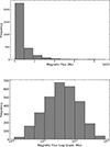 |
Fig. 1. Histogram of the total flux Φ of ARs on linear (left) and logarithmic (right) scales. |
For variables with a non-normal distribution, the median is expected to be more robust than using the mean. Hence, for each bin, we calculated the median value of the variable studied. We estimated the uncertainty of this value as  , where ni is the number of values in the bin and σi their standard deviations. Although this formula is strictly valid only for a normal distribution, the error introduced by this is considered admissible in view of the large extra computational burden that a proper bootstrap estimate would imply. This approximation nevertheless requires caution when evaluating fits with significantly non-Gaussian scatter and resulting in p-values that are not close to either 1 or 0.
3.1. Area versus flux
For the relation between flux and area, we show a log–log representation of the result in Fig. 2. A linear regression (dashed line) provides a very good representation of the data (χ2 = 1.83, p-value 0.78):
 (5)
(5)
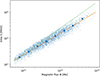 |
Fig. 2. Area A vs. magnetic flux Φ for ARs, with power law fits to the medians of the binned data (blue circles with error bars). The dashed line corresponds to the optimal fit; the dotted line shows a linear relationship A ∼ Φ for comparison. The lighter background shows a scatterplot of the individual points. |
where k = 0.836 ± 0.005, log CA = −15.21 ± 0.11, Φ is given in units of Mx, and A is given in MSH. The fit corresponds to a power-law dependence of the form A = CAΦk, with CA = 6.17 ⋅ 10−16, using the same units. The case k = 1 (dotted) is clearly excluded.
Fig. 3 displays the histogram of logarithmic residuals from Eq. (5). Despite a distinct negative skew (skewness −0.28), a Gaussian fit with a standard deviation of 0.1 provides a reasonable representation of the data. This implies that for a bipolar region of magnetic flux Φ, the logarithm of the area of the individual polarity patches is best represented as log A = ⟨log A⟩+rA, where ⟨log A⟩=klog Φ + log CA and rA is a Gaussian random variable with a standard deviation of 0.1.
We repeated the analysis by separating individual solar cycles; all cycles follow the scaling (5) without statistically significant deviations.
The power-law scaling found here is in good agreement with the findings of Meunier (2003), who reported Φ ∼ A1/k with 1/k ≃ 1.2 for the inverse relation. Other previous studies of the relationship between magnetic flux and area in solar ARs have reported linear scalings, i.e. k = 1 (Sheeley 1966; Wang & Sheeley 1989; van Driel-Gesztelyi & Green 2015; Muraközy 2024). However, these studies were mostly limited to sunspots, did not normally present statistical tests of goodness of fit, and the flux estimates used in the early studies were affected by large errors. rather crude.
Our result implies that the average field strength scales as Φ/A ∼ Φ0.16. While this is a mild increase, over the two orders of magnitude in flux covered by our sample (1021–1023 Mx) it still implies a factor of two increase in the average field amplitude. Whether this increase is due to a higher fraction of the area covered by spots or to a higher overall plage field strength is unclear. Further research will be required to clarify this issue.
3.2. Pole separation versus flux
Fig. 4 plots d against Φ for all ARs in the database. A logarithmic fit of the form
 (6)
(6)
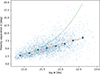 |
Fig. 4. Polarity separation d vs. logarithm of AR flux Φ. Median values are plotted for each bin (blue circles with error bars). The dashed line corresponds to a linear (i.e. logarithmic) fit. The dotted line shows the scaling d ∼ Φ1/2 for comparison. The lighter background shows a scatterplot of the individual points. |
provides a very good description of the data (χ2 = 0.8, p-value 0.997). The best-fit parameters obtained by linear regression are md = 3.32 ± 0.11 and Φ0 = 0.16 SFU. (The uncertainty in Φ0 is indirectly determined by the uncertainty of the intercept, as mdlog Φ0 = −2.64 ± 0.05.)
A small number of studies have considered the relation between Φ and d. Wang & Sheeley (1989), Tian et al. (2003), and Lemerle et al. (2015) all reported a power-law relationship, i.e. d ∼ Φm; however, the exponents obtained varied substantially, with values of m = 0.77, m = 0.87, and m = 0.42, respectively. This was based on a direct linear regression fit to an unbinned log–log scatterplot in all cases, and the goodness of fit was not determined. The high p-value obtained in our analysis clearly shows that a logarithmic fit is superior to the power-law fits. We note that a first indication of the logarithmic relationship can also be seen in Fig. 4 of Erofeev & Erofeeva (2023), based on white-light images, where the plotted relation between the logarithm of the total sunspot area in a sunspot group and the pole separation of clearly bipolar groups is not too far from linear.
Figure 5 presents the histogram of the fractional residuals rd = d/⟨d⟩ relative to the mean law given by Eq. (6). A lognormal fit provides a reasonably good representation of the data. Consequently, for a bipolar region of magnetic flux Φ, the pole separation may be best represented as d = rd ⋅ ⟨d⟩, where ⟨d⟩=mdlog(Φ/Φ0) as above, and log(rd) is a normally distributed random variable, with a standard deviation of 0.41.
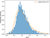 |
Fig. 5. Histogram of the fractional residuals d/⟨d⟩ relative to the linear fit in Fig. 4. The solid curve shows a lognormal fit. |
3.3. Tilt versus latitude (Joy’s law)
Table 1 summarises the bulk characteristics of the tilt distribution. The complete sample shows a clear preference for a tilt of γJ ∼ 7°, with the leading pole positioned closer to the equator, in accordance with Joy’s law. The numbers in the table align well with the findings of Qin et al. (2025) and place the ARISE sample among the higher-tilt ones, as discussed by Erofeev & Erofeeva (2023). This is in line (Wang et al. 2015) with the database used here being restricted to larger ARs with a clearly bipolar structure and good polarity balance. The discrepancies between data sets may also be related to the presence of magnetic tongues in plage structure (Poisson et al. 2020).
Bulk characteristics of the tilt in the sample.
Hemispheric asymmetry, as characterised by ⟨γ⟩, is not significant.
In contrast to area and pole separation, the tilt angle is primarily determined by heliographic latitude rather than flux (Joy’s law). To study this relation, we chose sin λ as an independent variable. This is motivated by the consideration that Joy’s law most plausibly originates from the Coriolis force, which scales with sin λ. We introduced nine bins; the bins have widths of 0.05, except for the lowest and highest bins, which comprise all ARs with |sin λ|< 0.1 and |sin λ|> 0.45, respectively.
Figure 6 presents the binned data with the Southern Hemisphere folded over the Northern one, that is, as a function of |sin λ|. A simple one-parameter linear regression of the form
 (7)
(7)
 |
Fig. 6. Tilt angle following Joy’s convention, γJ, vs. sine latitude for the complete sample. The dashed line corresponds to a homogeneous linear fit. |
provides a very good representation of the data (χ2 = 0.54, p-value 0.9998). We are thus unable to confirm occasional claims in the literature (McClintock & Norton 2013; Erofeev & Erofeeva 2023) of various nonlinearities in the shape of Joy’s law.
Separating the data by hemisphere or by solar cycle, we find no statistically significant differences in the value of the coefficient in Joy’s law. Our results for cycles 23 and 24 agree with the findings of Will et al. (2024) in that the value of mJ is higher in cycle 23 but the difference is not significant. The form of our fitting function, which is forced to go through the origin, may play a role in the lack of hemispheric asymmetry in our study. As recently pointed out by Zeng et al. (2024), the hemispheric asymmetry apparent in some studies is mostly due to low-latitude regions, and this would only show up when a non-zero intercept is allowed.
While the primary determinant of the tilt is clearly the latitude, some theoretical and empirical studies suggest that magnetic flux or AR size may play a secondary role (D’Silva & Howard 1993; Fan et al. 1994; Fisher et al. 1995; Sreedevi et al. 2024; Qin et al. 2025). In Fig. 7 we plot the slope mJ for subsamples divided into flux bins, as used in previous sections. (The top and bottom flux bins are not shown here, as some latitude bins contain too few points for reliable fits.) The plot suggests an increasing trend, but the null hypothesis of no dependence cannot be rejected with more than ∼1σ confidence, while the classic theoretical prediction mJ ∼ Φ1/4 (Fan et al. 1994) is clearly inconsistent with the data. If we use only three flux bins (with divisions at 2 and 7 SFU), the resulting Joy slopes in order of increasing flux are  ,
,  , and
, and  , respectively. The increasing trend is again suggestive, while the null hypothesis cannot be rejected at a confidence level much better than 1σ. This also illustrates the low sensitivity of our findings to the choice of binning, which is not demonstrated here in every case.
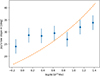 |
Fig. 7. Slope of Joy’s law determined for subsamples in different flux bins plotted against log Φ. The dashed line corresponds to an optimal fit of the form mJ ∼ Φ1/4, which is clearly inconsistent with the data. |
These inconclusive results help explain contradictory results in previous studies, some of which reported no correlation or even negative correlations of tilt with flux (Kosovichev & Stenflo 2008; McClintock & Norton 2016; Jha et al. 2020).
The standard deviation of the tilt values, on the other hand, displays a much clearer trend with magnetic flux (Fig. 8), significant at 6σ. A linear fit yields
 (8)
(8)
 |
Fig. 8. Standard deviation of tilt angles γJ vs. magnetic flux (top) and pole separation (bottom). The dashed lines correspond to linear end exponential fits, respectively. |
Given our above finding d ∼ log Φ, we also constructed a plot of σJ versus d (Fig. 8, right panel). The alignment of the points becomes even tighter in this case, possibly indicating that the geometry of the rising loop plays a more direct role in regulating deviations from Joy’s law. An exponential fit provides a convincing description of the relation (p-value 0.73):
 (9)
(9)
However, the stronger dependence of the scatter on d may be caused at least partially by a simple geometrical effect. For an uncertainty σp in the determination of the pole position, the error in tilt determination is σp/d, decreasing with separation. This effect may also contribute to the tighter alignment of the points in the lower panel.
We also note that the poorer alignment of the scatter with flux may be due to the lower precision of the flux determination. However, we do not consider this possibility highly likely, given that we carefully cross-checked the flux values in the ARISE catalogue by comparing MDI versus HMI data and against other catalogues (Wang et al. 2023). Furthermore, Fisher et al. (1995) reported a similarly tight relation between d and tilt scatter, even though their d values were determined from white light images only, implying significantly larger uncertainties. Finally, we note that Stenflo & Kosovichev (2012) reported a much stronger dependence of tilt scatter on Φ, but only for flux values in the range 0.1–1 SNU, below that studied here.
The distribution of residuals around Joy’s law remains to be determined. The decreasing trend of scatter around the law, Eq. (9), suggests using normalised residuals rJ = (γJ − ⟨γJ⟩)/σJ. We show the histogram of the rJ values obtained from Eq. (9) for σJ in Fig. 9. With this normalisation, the full sample collapses onto a nearly universal distribution.
 |
Fig. 9. Histogram of normalised residuals around Joy’s law. Optimally fitted Gaussian, Student’s t, and Laplace distributions are shown for comparison. |
To model this distribution, we first attempt to fit a Gaussian, which would be the natural expectation for tilt scatter resulting from random convective buffeting during flux emergence. Many such independent convective kicks should naturally result in a Gaussian distribution by virtue of the central limit theorem of probability theory. The Gaussian fit, however, can be rejected with a very high confidence (p-value of 3 ⋅ 10−8 based on a Kolmogorov–Smirnov test). Even by visual inspection, the distribution is distinctly non-Gaussian and leptokurtic, with a strong peak and extended tails (excess kurtosis +2.8). The high excess kurtosis is the hallmark of an intermittent stochastic perturbing process where most instances are only slightly perturbed (the strong peak), while in a small fraction of instances a single large perturbation results in large deviations (the tail). Standard methods in statistical physics for modelling such leptokurtic distributions resulting from intermittent processes include a double-exponential (or Laplace) distribution or a Student’s t-distribution. The Laplace distribution only marginally fits our data (p-value = 0.067), while a Student’s t-distribution with 3.7 degrees of freedom provides a satisfactory overall match (p-value 0.18). This agrees well with the findings of Muñoz-Jaramillo et al. (2021) that a t-distribution with 3.45 degrees of freedom represents the (unnormalised) tilt residuals well.
The presence of extended tails thus indicates that fluctuations are governed by intermittent, impulsive perturbations to the emerging flux tubes, rather than many small, independent Gaussian kicks. This type of distribution may be expected from sporadic convective buffeting, pre-existing magnetic structures, or episodic vortical forcing during emergence, as a result of which a small fraction of AR flux loops may be subjected to an intermittent large-amplitude torque during their rise.
However, the actual histogram of normalised residuals has a considerable skewness of −0.4. From visual inspection of Fig. 9, this asymmetry is primarily located in the tails, where negative residuals are more common than the fitted t-distribution, while positive residuals are less common. This suggests that AR flux tubes subjected to excessive disturbance prior to emergence tend to become completely oblivious of Joy’s law, their tilt distribution becoming more symmetrical to the equator.
In summary, we suggest that for a bipolar region of magnetic flux Φ emerging at latitude λ, the tilt angle γJ is best represented as ⟨γJ⟩+rJσJ, where rJ is a random variable with a distribution described by a Student’s t-distribution of 3.7 degrees of freedom, and σJ is obtained from Eq. (9) (or alternately from Eq. (8), in which case a t-function with 2.9 degrees of freedom is to be used). For applications where an accurate representation of the tails of the distribution is important, accounting for the skewness by suppressing (amplifying) the positive (negative) tail of the distribution may be considered.
4. Discussion
4.1. Evolutionary effects
Active regions evolve throughout their life, which implies that all the quantities studied depend on time (van Driel-Gesztelyi & Green 2015, Forgács-Dajka et al. 2021). The AR data listed in the ARISE catalogue were obtained from synoptic maps. On these maps, ARs are captured on the day of their central meridian passage, i.e. at a random instant during their evolution. It is therefore not necessarily trivial to link, for example, the measured value of the flux Φ to its maximal value Φ0, which presumably corresponds to the physically meaningful total magnetic flux in the rising magnetic flux loop. Other parameters such as d or γ may not display a maximum during their evolution, but some characteristic values corresponding to a particular evolutionary phase (e.g. when Φ attains its maximum) may still be defined. The question therefore arises as to what extent the scaling relations derived above remain valid for the more meaningful underlying parameters Φ0, d0, etc.
Fortunately, there is some evidence that the parameter evolution curves of ARs exhibit a certain universality, that is, for any observable y,
 (10)
(10)
where the AR lifetime is given by T = f(Φ0) and the function fy(x) is a universal average AR evolution curve for the observable y. Švanda et al. (2025) recently determined these average curves for different observables up to a time shortly after flux maximum for 36 ARs. The curves are generally consistent with the findings of previous studies with a narrower focus or smaller samples (Kosovichev & Stenflo 2008; Schunker et al. 2019; Will et al. 2024).
Assuming universality, the expected value of an observable measured at a random instant on synoptic maps scales linearly with the characteristic value y0:
 (11)
(11)
This suggests that the scalings found in this work may also be valid for the underlying characteristic scales, with scatter resulting from a combination of evolutionary phase and real physical scatter.
Despite the evidence for a universal average behaviour, some doubts regarding its validity remain, especially in the case of the tilt (McClintock & Norton 2016). More extensive studies of AR evolution are needed to clarify this issue. Studies such as Schunker et al. (2020) and the AutoTAB catalogue compiled by Sreedevi et al. (2023) are important steps in this direction.
4.2. Implications for AR formation
Fan (2021) and Weber et al. (2023) review models and concepts for the subsurface origin of ARs. The classic paradigm of the buoyant rise of a flux loop from the bottom of the convective zone to near-surface layers remains the only coherent scenario (Petrovay & Christensen 2010) worked out in numerical detail. Alternative possibilities include originating depths in the bulk of the convection zone or in the near-surface shear layer, as well as the rise driven by the drag of convective upflows (see e.g. Birch et al. 2016, Hotta & Iijima 2020, and Chen et al. 2022).
Predictions of AR scaling laws from these models have focused on Joy’s law. Proposed explanations for the origin of this law include the following.
-
(1)
The tilt may reflect the orientation of the underlying flux tubes that give rise to the emerging loops. The orientation of these tubes, which originate from the winding-up of the seed poloidal field present at solar minimum, may be inclined to the azimuthal direction. (Babcock 1961; Norton & Gilman 2005; Tlatova et al. 2018)
-
(2)
The tilt forms during the rise of the flux loop through the convective zone due to the action of Coriolis force on:
-
(a)
flows inside the loop, whose rise is driven by magnetic buoyancy (D’Silva & Choudhuri 1993; Caligari et al. 1995; Weber et al. 2013, among others)
-
(b)
helical convective flows that distort the loop (and possibly contribute to its rise) through drag (the ‘Σ-effect’; Longcope et al. 1998)
-
(a)
-
(3)
The tilt may form during and/or after the emergence of the flux loop through the surface due to the effect of supergranular flows affected by the Coriolis force (Roland-Batty et al. 2025, Schunker & K V 2025).
In the classic model of the origin of ARs, sometimes called the ‘buoyant thin flux tube paradigm’, the underlying toroidal field lies in the tachocline, at or slightly below the bottom of the convective zone. In such models several independent lines of evidence point to an initial field strength of B0 ∼ 105 G (see Petrovay & Christensen 2010 for a summary of these arguments). Such models (Fan et al. 1994) predict a tilt scaling of γJ ∼ Φ1/4B0−5/4. Evidence for this dependence would provide strong support for the thin flux tube model. However, as discussed in Sect. 3.3, the observed flux dependence of the tilt is much weaker than the predicted Φ1/4 dependence. This is not necessarily inconsistent with the classic model, as the initial field strength may also vary and there may be a statistical relation between Φ and B0. Indeed, as discussed in Sect. 3.1, our A–Φ relation implies such a relation between the flux of an AR and its mean magnetic field in the photospheric layers.
Regarding the pole separation d, observations of AR evolution generally indicate that after an initial rapid increase, d saturates at a constant value of ∼100 Mm (Kosovichev & Stenflo 2008; Schunker et al. 2019; Švanda et al. 2025). Indeed, recurrent sunspot groups are often observed to return several times with the position of the polarities changing very little. This is surprising in the context of the buoyant flux loop paradigm, as the most unstable modes tend to be those with low wavenumber m, corresponding to scales of 300 Mm or longer. The observed length scales are closer to the scales of turbulent convection in the deep convective zone, predicted by mixing-length models and numerical simulations, which are determined by the scale height. This may indicate that the typical scale of finite-amplitude initial perturbations plays a more important role in determining the size of rising flux loops. The puzzling but robust logarithmic scaling of d with Φ discovered in our analysis may provide important clues regarding the turbulence spectra in the deep convective zone and the depths of origin of the rising flux loops.
5. Conclusion
We analysed the recently compiled ARISE database of solar bipolar magnetic regions to study how geometric AR parameters scale with the fundamental parameter, magnetic flux Φ. The geometric parameters studied were: area A, pole separation d, and tilt angle γJ.
Our most novel finding is that, contrary to what was found (or, rather, a priori assumed) in previous studies, the d–Φ relation is not a power law but a well-determined and highly robust logarithmic relation. The scaling of A with Φ deviates from linear, implying that the mean field strength increases with region size. For the tilt angle, we find that the slope of Joy’s law shows a tendency to increase with Φ but the significance of this result is low and the trend is much weaker than the theoretical prediction γJ ∼ Φ1/4. The scatter around Joy’s law decreases linearly with Φ and exponentially with d.
We also studied the distribution of residuals around the mean scaling laws. We find A and d to be roughly lognormally distributed, while we confirm the earlier finding that residuals from Joy’s law follow a Student’s t-distribution with ∼3.5 degrees of freedom. These scalings and residual distributions allow us to construct a recipe for the synthesis of an ensemble or population of ARs that correctly reflects the observed statistics. We summarise this recipe in the appendix by collecting the relevant fitting formulae from the main text.
Acknowledgments
This research was supported by the European Union’s Horizon 2020 research and innovation programme under grant agreement No. 955620 and by the NKFIH excellence grant TKP2021-NKTA-64. RE is also grateful to the Hungarian National Research, Development and Innovation Fund (NKFIH, grant no. K142987); the UK Science and Technology Facilities Council (STFC, grant no. ST/M000826/1); PIFI (China, grant no. 2024PVA0043). RHW is supported by the National Natural Science Foundation of China (grant No. 12425305).
References
- Babcock, H. W. 1961, ApJ, 133, 572 [Google Scholar]
- Bhowmik, P., Jiang, J., Upton, L., Lemerle, A., & Nandy, D. 2023, Space Sci. Rev., 219, 40 [NASA ADS] [CrossRef] [Google Scholar]
- Birch, A. C., Schunker, H., Braun, D. C., et al. 2016, Sci. Adv., 2, e1600557 [CrossRef] [Google Scholar]
- Caligari, P., Moreno-Insertis, F., & Schussler, M. 1995, ApJ, 441, 886 [Google Scholar]
- Chen, F., Rempel, M., & Fan, Y. 2022, ApJ, 937, 91 [NASA ADS] [CrossRef] [Google Scholar]
- D’Silva, S., & Choudhuri, A. R. 1993, A&A, 272, 621 [NASA ADS] [Google Scholar]
- D’Silva, S., & Howard, R. F. 1993, Sol. Phys., 148, 1 [Google Scholar]
- Erofeev, D. V., & Erofeeva, A. V. 2023, Geomagn. Aeron., 63, 1007 [Google Scholar]
- Fan, Y. 2021, Liv. Rev. Sol. Phys., 18, 5 [NASA ADS] [CrossRef] [Google Scholar]
- Fan, Y., Fisher, G. H., & McClymont, A. N. 1994, ApJ, 436, 907 [Google Scholar]
- Fisher, G. H., Fan, Y., & Howard, R. F. 1995, ApJ, 438, 463 [NASA ADS] [CrossRef] [Google Scholar]
- Forgács-Dajka, E., Dobos, L., & Ballai, I. 2021, A&A, 653, A50 [NASA ADS] [CrossRef] [EDP Sciences] [Google Scholar]
- Harvey, K. L., & Zwaan, C. 1993, Sol. Phys., 148, 85 [Google Scholar]
- Hotta, H., & Iijima, H. 2020, MNRAS, 494, 2523 [Google Scholar]
- Jha, B. K., Karak, B. B., Mandal, S., & Banerjee, D. 2020, ApJ, 889, L19 [NASA ADS] [CrossRef] [Google Scholar]
- Kosovichev, A. G., & Stenflo, J. O. 2008, ApJ, 688, L115 [NASA ADS] [CrossRef] [Google Scholar]
- Lemerle, A., Charbonneau, P., & Carignan-Dugas, A. 2015, ApJ, 810, 78 [NASA ADS] [CrossRef] [Google Scholar]
- Leussu, R., Usoskin, I. G., Senthamizh Pavai, V., et al. 2017, A&A, 599, A131 [NASA ADS] [CrossRef] [EDP Sciences] [Google Scholar]
- Longcope, D. W., Fisher, G. H., & Pevtsov, A. A. 1998, ApJ, 507, 417 [NASA ADS] [CrossRef] [Google Scholar]
- McClintock, B. H., & Norton, A. A. 2013, Sol. Phys., 287, 215 [NASA ADS] [CrossRef] [Google Scholar]
- McClintock, B. H., & Norton, A. A. 2016, ApJ, 818, 7 [NASA ADS] [CrossRef] [Google Scholar]
- Meunier, N. 2003, A&A, 405, 1107 [NASA ADS] [CrossRef] [EDP Sciences] [Google Scholar]
- Muñoz-Jaramillo, A., Senkpeil, R. R., Windmueller, J. C., et al. 2015, ApJ, 800, 48 [Google Scholar]
- Muñoz-Jaramillo, A., Navarrete, B., & Campusano, L. E. 2021, ApJ, 920, 31 [Google Scholar]
- Muraközy, J. 2024, A&A, 690, A257 [NASA ADS] [CrossRef] [EDP Sciences] [Google Scholar]
- Norton, A. A., & Gilman, P. A. 2005, ApJ, 630, 1194 [NASA ADS] [CrossRef] [Google Scholar]
- Petrovay, K. 2020, Liv. Rev. Sol. Phys., 17, 2 [Google Scholar]
- Petrovay, K., & Christensen, U. R. 2010, Space Sci. Rev., 155, 371 [Google Scholar]
- Poisson, M., Démoulin, P., Mandrini, C. H., & López Fuentes, M. C. 2020, ApJ, 894, 131 [NASA ADS] [CrossRef] [Google Scholar]
- Qin, L., Jiang, J., & Wang, R. 2025, ApJ, 986, 114 [Google Scholar]
- Roland-Batty, W., Schunker, H., Cameron, R. H., et al. 2025, A&A, 700, A28 [NASA ADS] [CrossRef] [EDP Sciences] [Google Scholar]
- Schunker, H., & K V, A. L., 2025, Sol. Phys., 300, 161 [Google Scholar]
- Schunker, H., Birch, A. C., Cameron, R. H., et al. 2019, A&A, 625, A53 [NASA ADS] [CrossRef] [EDP Sciences] [Google Scholar]
- Schunker, H., Baumgartner, C., Birch, A. C., et al. 2020, A&A, 640, A116 [NASA ADS] [CrossRef] [EDP Sciences] [Google Scholar]
- Seiden, P. E., & Wentzel, D. G. 1996, ApJ, 460, 522 [Google Scholar]
- Sheeley, N. R., Jr. 1966, ApJ, 144, 723 [NASA ADS] [CrossRef] [Google Scholar]
- Sreedevi, A., Jha, B. K., Karak, B. B., & Banerjee, D. 2023, ApJS, 268, 58 [Google Scholar]
- Sreedevi, A., Jha, B. K., Karak, B. B., & Banerjee, D. 2024, ApJ, 966, 112 [Google Scholar]
- Stenflo, J. O., & Kosovichev, A. G. 2012, ApJ, 745, 129 [NASA ADS] [CrossRef] [Google Scholar]
- Švanda, M., Jurčák, J., & Schmassmann, M. 2025, A&A, 700, A40 [NASA ADS] [CrossRef] [EDP Sciences] [Google Scholar]
- Tian, L., Liu, Y., & Wang, H. 2003, Sol. Phys., 215, 281 [Google Scholar]
- Tlatova, K., Tlatov, A., Pevtsov, A., et al. 2018, Sol. Phys., 293, 118 [NASA ADS] [CrossRef] [Google Scholar]
- van Driel-Gesztelyi, L., & Green, L. M. 2015, Liv. Rev. Sol. Phys., 12, 1 [Google Scholar]
- Wang, Y. M., & Sheeley, N. R., Jr. 1989, Sol. Phys., 124, 81 [NASA ADS] [CrossRef] [Google Scholar]
- Wang, Y. M., Colaninno, R. C., Baranyi, T., & Li, J. 2015, ApJ, 798, 50 [Google Scholar]
- Wang, R., Jiang, J., & Luo, Y. 2023, ApJS, 268, 55 [NASA ADS] [CrossRef] [Google Scholar]
- Wang, R., Jiang, J., & Luo, Y. 2024, ApJ, 971, 110 [Google Scholar]
- Weber, M. A., Fan, Y., & Miesch, M. S. 2013, Sol. Phys., 287, 239 [NASA ADS] [CrossRef] [Google Scholar]
- Weber, M. A., Schunker, H., Jouve, L., & Işık, E. 2023, Space Sci. Rev., 219, 63 [NASA ADS] [CrossRef] [Google Scholar]
- Will, L. W., Norton, A. A., & Hoeksema, J. T. 2024, ApJ, 976, 20 [Google Scholar]
- Yeates, A. R., Cheung, M. C. M., Jiang, J., Petrovay, K., & Wang, Y.-M. 2023, Space Sci. Rev., 219, 31 [CrossRef] [Google Scholar]
- Zeng, S.-G., Zhao, A.-Y., Yi, S., et al. 2024, ApJ, 975, 210 [Google Scholar]
For readers less familiar with magnetic data: northern and southern polarity refers to the directionality of magnetic field lines and is not related to heliographic latitude.
Appendix A: Active region population synthesis: A recipe
Surface flux transport models, widely used to compute the evolution of the Sun’s large scale magnetic field, include ARs as a source term (Yeates et al. 2023). This source often needs to be modelled to account for missing data or future evolution: it is clearly important for any such model to be as realistic as possible.
In what follows we give a concise summary of the relevant findings in our paper in the form of a ‘recipe’ to generate an ensemble of ARs to be used as source term in an SFT or dynamo model. Prescribing when, where and with what magnetic flux a bipolar region will emerge in such models is beyond the scope of the present work. We restrict our attention to determining the area A of the individual flux patches; their separation d; and the tilt angle of the bipole axis.
For a bipolar region of magnetic flux Φ emerging at latitude λ:
(1) The logarithm of the area A of the individual polarity patches is best represented as log A = ⟨log A⟩+rA where
![Mathematical equation: $$ \begin{aligned} \langle \log A \text{[MSH]}\rangle = k\log \Phi \text{[Mx]} +\log C_A \end{aligned} $$](/articles/aa/full_html/2026/06/aa59071-26/aa59071-26-eq19.gif) (A.1)
(A.1)
with k = 0.84 and CA = 6.17 ⋅ 10−16 , while rA is a Gaussian random variable with standard deviation 0.1.
(2) The pole separation may be best represented as d = rd ⋅ ⟨d⟩, where
 (A.2)
(A.2)
with  and Φ0 = 1.6 ⋅ 1020 Mx, while log(rd) is a normally distributed random variable, with standard deviation 0.41.
(3) The tilt angle γJ is best represented as ⟨γJ⟩+rJσJ where
 (A.3)
(A.3)
while rJ is a random variable with a distribution described by Student’s t-distribution of 3.7 degrees of freedom, and σJ is obtained from
 (A.4)
(A.4)
or alternately from
![Mathematical equation: $$ \begin{aligned}&\sigma _J =a+b\log (\Phi \text{[SFU]}) \quad \text{ with} \\&a = 25{\overset{\circ }{.}}57 \quad \text{ and} \quad b = 3{\overset{\circ }{.}}75 \nonumber \end{aligned} $$](/articles/aa/full_html/2026/06/aa59071-26/aa59071-26-eq24.gif) (A.5)
(A.5)
in which case a t-function with 2.9 degrees of freedom is to be used.
For applications where an accurate representation of the tails of the distribution matters, accounting for the skewness by suppressing [amplifying] the positive [negative] tail of the distribution may be considered.
All Tables
All Figures
|
Fig. 1. Histogram of the total flux Φ of ARs on linear (left) and logarithmic (right) scales. |
| In the text | |
|
Fig. 2. Area A vs. magnetic flux Φ for ARs, with power law fits to the medians of the binned data (blue circles with error bars). The dashed line corresponds to the optimal fit; the dotted line shows a linear relationship A ∼ Φ for comparison. The lighter background shows a scatterplot of the individual points. |
| In the text | |
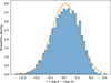 |
Fig. 3. Histogram of residuals from the fit in Fig. 2. The solid line shows a Gaussian fit. |
| In the text | |
|
Fig. 4. Polarity separation d vs. logarithm of AR flux Φ. Median values are plotted for each bin (blue circles with error bars). The dashed line corresponds to a linear (i.e. logarithmic) fit. The dotted line shows the scaling d ∼ Φ1/2 for comparison. The lighter background shows a scatterplot of the individual points. |
| In the text | |
|
Fig. 5. Histogram of the fractional residuals d/⟨d⟩ relative to the linear fit in Fig. 4. The solid curve shows a lognormal fit. |
| In the text | |
|
Fig. 6. Tilt angle following Joy’s convention, γJ, vs. sine latitude for the complete sample. The dashed line corresponds to a homogeneous linear fit. |
| In the text | |
|
Fig. 7. Slope of Joy’s law determined for subsamples in different flux bins plotted against log Φ. The dashed line corresponds to an optimal fit of the form mJ ∼ Φ1/4, which is clearly inconsistent with the data. |
| In the text | |
|
Fig. 8. Standard deviation of tilt angles γJ vs. magnetic flux (top) and pole separation (bottom). The dashed lines correspond to linear end exponential fits, respectively. |
| In the text | |
|
Fig. 9. Histogram of normalised residuals around Joy’s law. Optimally fitted Gaussian, Student’s t, and Laplace distributions are shown for comparison. |
| In the text | |
Current usage metrics show cumulative count of Article Views (full-text article views including HTML views, PDF and ePub downloads, according to the available data) and Abstracts Views on Vision4Press platform.
Data correspond to usage on the plateform after 2015. The current usage metrics is available 48-96 hours after online publication and is updated daily on week days.
Initial download of the metrics may take a while.