| Issue |
A&A
Volume 709, May 2026
|
|
|---|---|---|
| Article Number | A30 | |
| Number of page(s) | 11 | |
| Section | Numerical methods and codes | |
| DOI | https://doi.org/10.1051/0004-6361/202558060 | |
| Published online | 29 April 2026 | |
Nemesis: A multi-scale, multi-physics algorithm for astrophysics
Leiden Observatory, University of Leiden,
Niels Bohrweg 2,
2333
CA
Leiden,
The Netherlands
★ Corresponding author: This email address is being protected from spambots. You need JavaScript enabled to view it.
Received:
11
November
2025
Accepted:
10
March
2026
Abstract
Context. Astronomical environments are governed by a complex interplay of physical processes, including gravitational dynamics, radiative transfer, stellar evolution, chemistry, and hydrodynamics. These processes span a vast range of spatial scales, from short-range interactions where intra-particle distances are vital, to cosmological scales. Both of these characteristics make astrophysics a multi-scale, multi-physics discipline. This complexity introduces complications to numerical methods where round-off errors and a wide range of temporal timescales on which processes act can influence the reliability of results and the efficiency of algorithms.
Aims. In this work, we present an updated version of the multi-scale, multi-physics algorithm, Nemesis, which makes use of the Astrophysical Multipurpose Software Environment (AMUSE). We formally introduce and validate the algorithm.
Methods. We ran a suite of simulations to assess its performance in simulating star clusters containing planetary systems, its ability to capture the von Zeipel–Lidov–Kozai effect, and its computational scalability.
Results. The Nemesis code yields indistinguishable results on both the global and local scales when compared with the direct N-body code Ph4. We find the same result when analysing its ability to capture the von Zeipel–Lidov–Kozai effect. When we analyse its computational performance, the wall-clock time scales roughly as tsim ∝ 1/ δtnem, where δtnem represents the time synchronisation between the global and local scales. When we vary the number of planetary systems, the wall-clock time remains unchanged as long as the number of available cores exceeds the number of systems. Beyond this, we find that, at worst, the computational time increases linearly with the number of excess systems.
Conclusions. The method introduced here can be used in numerous domains of astronomy, thanks to its flexibility and modularity, from simulating protoplanetary discs in star clusters to binary black holes in the galactic centre.
Key words: methods: numerical / planets and satellites: dynamical evolution and stability / planet-disk interactions / planet-star interactions / planetary systems
© The Authors 2026
 Open Access article, published by EDP Sciences, under the terms of the Creative Commons Attribution License (https://creativecommons.org/licenses/by/4.0), which permits unrestricted use, distribution, and reproduction in any medium, provided the original work is properly cited.
This article is published in open access under the Subscribe to Open model. This email address is being protected from spambots. You need JavaScript enabled to view it. to support open access publication.
1 Introduction
In the early eighties, it was proposed that the Sun had a distant companion, ‘Nemesis’. The Nemesis hypothesis helped to explain the apparent periodic epochs of extinction found in the fossil records (Whitmire & Jackson 1984; Davis et al. 1984). Its existence has since been ruled out by infrared observations (Kirkpatrick et al. 2011) and by additional data analysis showing that the mass-extinction events are, in fact, not periodic (Bailer-Jones 2011). Nevertheless, the notion that such a distant body can be perceived as a companion highlights the multi-scale nature of astronomy. Compared to the 88 days that Mercury takes to orbit the Sun, Nemesis would take ~1010 days (Whitmire & Jackson 1984), roughly the orbital period of the Sun around the galactic centre.
The multi-scale nature of astronomy complicates matters in computational astrophysics. A wide range in mass and length (i.e. stars orbiting a supermassive black hole or clusters orbiting the galaxy) introduces numerical round-off errors (Boekholt & Portegies Zwart 2015). These numerical errors may grow exponentially in chaotic N-body systems (Poincaré 1891, 1892; Dejonghe & Hut 1986), resulting in divergent evolutionary histories. The matter is further complicated, as a wide range in length can also translate to a wide range in characteristic times for dynamical systems. For instance, while a planet may orbit its host on timescales of months or even days, a young stellar cluster has crossing times of ~1 Myr and may dissolve in the galactic tidal field on timescales of 100 Myr (Portegies Zwart et al. 2010). This multi-scale nature in dynamical systems has led to the development of various N-body integration strategies over the decades, with each implementing its own schemes and approximations depending on the problem at hand (see, e.g. Heggie (2003) for a review):
Statistical methods (Spitzer & Hart 1971; Hénon 1971; Cohn 1979; Giersz 1998; Spurzem et al. 2005): statistical approaches such as Monte Carlo simulations, the anisotropic gaseous models, or Fokker–Planck methods are well suited for integrating systems that satisfy certain symmetries, such as globular clusters. However, their statistical nature yields poor solutions when resolving tight encounters or systems where spherical symmetry is no longer applicable.
Tree codes (Barnes & Hut 1986): tree codes compute pairwise gravitational forces between nearby particles, but approximate those between particles with larger separations. This method is designed for large N problems, namely galactic and cosmological simulations, scaling as 𝒪(N log N), with N being the number of simulated particles. However, approximating long-range forces makes them ill-suited to resolving collisional systems, where tight energy conservation is required to ensure that interactions are accurately resolved.
Direct N-body codes: these codes compute all pairwise forces. Their 𝒪(N2) scaling makes them less efficient at large N relative to the previous two families, but techniques such as regularisation (Stiefel & Kustaanheimo 1965; Aarseth & Zare 1974), individual time steps or the Ahmad-Cohen scheme (Ahmad & Cohen 1973; Makino & Aarseth 1992) mitigate these bottlenecks making them optimised for cluster dynamics. These same approximations affect the smallest scales and do not yield time-symmetric solutions. Following Noether (1918), without time-symmetry, a drift in energy error occurs, artificially altering a system’s dynamics over secular timescales.
Symplectic codes (Wisdom & Holman 1991): symplectic codes provide time-symmetric solution, as their equations map directly from the system’s Hamiltonian. As a result, symplectic codes are ideal for simulating planetary systems over long timescales. Nevertheless, their time-symmetric nature requires all particles to share the same time step. Constrained by the tightest orbit, symplectic codes perform poorly beyond moderate N systems.
Hybrid codes attempt to combine different families to best fit a given problem. For instance, LonelyPlanets (Cai et al. 2017) adopts a two-step process to integrate planetary systems in star clusters, using both a symplectic code for its planetary orbits and a direct N-body code for the cluster evolution. Meanwhile, codes such as P3T (Iwasawa et al. 2015), PeTar (Wang et al. 2020) and Ketju (Rantala et al. 2017; Mannerkoski et al. 2023) couple tree code-like schemes with direct N-body integration to enable optimised simulations of galactic environments, with special attention to the galactic core.
The multi-physics discipline of astronomy adds another layer of complexity. For brevity, consider only a star cluster in which not all the gas within a molecular cloud contributes to star formation. Observations of the solar neighbourhood indicate that approximately 10–35% of the gas in a molecular cloud convert into stars (Lada & Lada 2003; Lada et al. 2010), while the rest remains embedded in the cluster, deepening the potential well and thereby affecting the stellar dynamics. Once the first supernova occurs, this gas is expelled, and the resulting impulsive mass loss alters the cluster potential, driving rapid expansion (Hills 1980) and reshaping the gravitational potential, both of which influence the stellar dynamics. The influence of stellar evolution on dynamics is also apparent during a star’s lifetime, as mass loss via stellar winds heats the cluster, causing both expansion of the system and a reduction in the gravitational strength between stars. Beyond dynamics, stellar evolution also regulates the radiation field, which, for instance, controls the evaporation rate of protoplanetary discs and subsequently affects the growth of planets (see e.g. Winter et al. 2022; Wilhelm et al. 2023; Huang et al. 2024). These simple examples illustrate the extent to which gravitational, hydrodynamical, and radiative processes are intertwined in astronomy. Ignoring feedback between frameworks in astronomy risks oversimplifying problems, and while challenging to implement numerically, including multi-physics in numerical models provides both more faithful and more predictive results.
In this paper, we formally present a hybrid technique capable of handling multi-physics problems: Nemesis1. This technique was previously used to integrate planetary systems in star clusters (van Elteren et al. 2019); here, we provide a more detailed description and validation of the recently modified and optimised version. Results show that the core approximation on which Nemesis is built, that is, decoupling widely separated systems from each other and solving them in parallel, yields negligible loss in physics while providing massive computational benefits. The flexibility of this hybrid code allows researchers to tackle multi-scale and multi-physics problems.
2 Theory of Nemesis
The Nemesis code is developed within the AMUSE framework (Portegies Zwart et al. 2009; Pelupessy et al. 2013; Portegies Zwart & McMillan 2018). Currently, Nemesis is an external module and is not yet officially part of the AMUSE distribution. We intend to incorporate it into the main library in the future.
The AMUSE framework contains codes that can model different physical domains, such as stellar evolution, gravitational dynamics, astrochemistry, hydrodynamics, and radiative transfer. Within each domain, users can choose from multiple solvers, which offers considerable freedom in tailoring simulations to specific scientific goals. A full list of available codes within AMUSE is provided in Appendix B of Portegies Zwart & McMillan (2018).
This flexibility also benefits Nemesis, as it is designed to handle multi-physics problems with modularity. This is achieved via channels (van Elteren et al. 2014), which communicate data between codes, allowing processes within one physical domain to influence another. The AMUSE framework manages communication internally using the Message Passing Interface (MPI) (Gropp et al. 1996), which helps minimise overhead during data transfer. Although Nemesis is general-purpose, its original motivation was to solve planetary systems in star clusters. The following discussion primarily considers this context.
2.1 Managing multiple scales
As mentioned in the introduction, the wide range of timescales present in star clusters containing planetary systems introduces challenges in computational astronomy. Although direct N-body algorithms can handle moderate-to-large N systems, their various approximations introduce energy drift, leading to unreliable solutions over secular timescales. This is especially problematic in environments where subsystems exist (e.g., planetary systems or binary stars) since these tighter systems evolve much faster than the larger-scale environment they inhabit. Symplectic codes enable accurate results over secular timescales; however, their shared time-step scheme makes them inefficient for large N, as the tightest orbit halts all progress.
This clear separation between the characteristic evolutionary times of subsystems and the global environment decouples the problem, integrating each component in isolation and synchronising their states at regular intervals. As long as the synchronisation interval is short enough to capture essential interactions, the approximation holds. This separation motivates a hierarchical treatment of the environment, where global and local dynamics evolve independently. We introduce the following terminology to describe this framework:
Children: In Nemesis ‘children’ represent subsystems. That is, the set of particles lying within some distance of one another (see Section 2.3). A ‘child system’ can therefore correspond, for example, to a planetary system, a binary, or a triple. Within each child system, the individual particles (e.g., planets or stars) are referred to as ‘child particles’.
Child code: the ‘child code’ is the dedicated integrator assigned to a child system. Since each child system is integrated with its own code, users can ensure high energy conservation (e.g., by choosing a symplectic integrator). Additionally, this makes the scheme naturally parallelisable, as child codes can be distributed across CPU cores, reducing run time.
Parent: ‘parents’ are the set of particles tracked in the global environment. A parent particle represents either an isolated object (e.g., a single star or an interstellar object) or serves as a centre-of-mass (CoM) proxy of a child system.
Parent code: the ‘parent code’ is the integrator used to track the global evolution of the set of parent particles.
Representing a child system with a CoM proxy ensures that tight orbits are removed from the parent code, bypassing the poor resolution of tight systems within a direct N-body integration while still preserving the optimised performance of the integrator for moderate-to-large N systems.
Over time, the number of children, Nchd, can vary. During the parent integration, close encounters create a new child system. Conversely, a child system dissolves if any of its members become sufficiently separated (i.e., an ionising event between a binary and an intruder occurs). If Nchd exceeds the number of available cores, excess children wait in a queue until a CPU becomes available. The CPUs are released as soon as a child code finishes integrating, with priority given to the most computationally expensive jobs.
2.2 Synchronising scales
Since children are isolated from the global environment, neither scale communicates its dynamical history to the other. To ensure feedback across scales, Nemesis applies gravitational correction kicks between parents and children at regular time intervals, referred to as the bridge time step, δtnem. These kicks compensate for the fact that the parent code, represents children using a CoM proxy. While this approximation reduces computational cost, it alters the underlying potential during the parent integration step. Correction kicks restore missing forces in two ways:
-
Correction on parents: each parent receives a correction equal to the difference between the gravitational force exerted by all child particles within a system and that of its representative parent. Formally,
![Mathematical equation: $\[F_{\text {corr. par}, i}=\sum_{j=0, j \neq i}^{N_{\text {chd }}}\left(\sum_{k=0}^{n_{\text {chd }}} F_k-F_{\text {par}, j}\right),\]$](/articles/aa/full_html/2026/05/aa58060-25/aa58060-25-eq2.png) (1)
(1)where Fcorr.par, i is the correction force applied to parent i, Fk are the forces exerted by child particles contained within system j, and Fpar,j is the force from the parent representative of child system j (i.e. the CoM representative integrated in the parent code). This correction is summed over all children, Nchd. The condition j ≠ i ensures that a parent does not consider its own child system, as their dynamics are already accounted for in its phase-space representation.
For a virialised Plummer sphere with density ρ ~ 102 M⊙ pc−3, when ten out of 200 stars host planetary systems, applying these corrections over bridge time steps of 500 yr results in a kick of δv ~ 10−17 km s−1. Increasing the density to 103 M⊙ pc−3 and the number of planetary systems to 100 out of 2000, the corrections become δv ~ 10−13 km s−1.
Although the corrections are minor, they accumulate over time. Moreover, as mentioned earlier, large N systems are inherently chaotic. As such, including these corrections may translate into subtle but distinct dynamical effects.
-
Correction on children: each child particle receives a correction equal to the difference between the total force from all external parents and the force from its own parent. Formally,
![Mathematical equation: $\[F_{\text {corr. chd}, j}=\sum_{j=0}^{N_{\mathrm{chd}}}\left(\sum_{k=0, k \neq j}^{N_{\mathrm{par}}} F_k-F_{\mathrm{par}, j}\right),\]$](/articles/aa/full_html/2026/05/aa58060-25/aa58060-25-eq3.png) (2)
(2)where Fcorr.chd,j is the gravitational correction applied to all child particles within system j, Fk is the force from all external parents, and Fpar,j is the parent of system j.
As before, for context, we consider a virialised Plummer sphere with density 100 M⊙ pc−3, in which ten of 200 host planetary systems. The corrections applied to the planets over the same 500 year bridge time steps result in velocity shifts of δv ~ 10−10–10−7 km s−1. The large spread arises from the sensitivity of the local environment, since gravity follows an inverse-squared law with spatial separations. When ρ ~ 103 M⊙ pc−3, this ranges between δv ~ 10−8–10−5 km s−1.
The code applies correction kicks every bridge time step using a second-order Verlet kick–drift–kick method (Verlet 1967; Fujii et al. 2007). In the limit δtnem → 0 yr, Nemesis mimics a direct second-order N-body integrator, albeit with substantial overhead. In the opposite limit, δtnem → ∞ yr, computational time is minimised, but accuracy is lost.
The only interaction not considered in Nemesis is between members of distinct children. Concretely, particles within one planetary system do not influence particles within another planetary system. These particles interact only through their parent proxies. Given this, the distance criterion for forming a child system should remain small relative to the interparticle distance. This enhances the validity of the CoM approximation and minimises situations where several comparable-mass particles reside in the same child system, since such configurations reduce the accuracy of the CoM approximation.
Once a particle is no longer identified as a child, for example, when it is ejected and becomes a rogue planet, it becomes a parent. Its dynamical evolution is then treated in the parent code and it feels the effects of all remaining children through correction kicks (see Section 2.4).
2.3 Handling parent mergers
At times, two parents will be near enough that their internal dynamics require a more accurate resolution. The collision detection stopping condition in AMUSE detects such events by checking at every internal time step whether two parents are spatially separated by less than the sum of their collisional radii. In Nemesis, a parent’s collisional radius is defined as
![Mathematical equation: $\[R_{\mathrm{par}}=A\left(\frac{M_{\mathrm{par}}}{\mathrm{M}_{\odot}}\right)^{1 / 3} \mathrm{au}.\]$](/articles/aa/full_html/2026/05/aa58060-25/aa58060-25-eq4.png) (3)
(3)
Here, A is a user-defined coefficient (default A = 100) and Mpar is the mass of the parent. For isolated parents (i.e., parents hosting no children, such as a rogue planet or single star), Mpar is the particle’s mass. If the parent instead hosts children, Mpar is the total mass of the child system. By default, the code applies an upper limit of Rpar = 103 au. While test particles are massless and therefore have no radii, isolated test particles can still merge upon the approach of another (massive) parent particle. The Nemesis code handles mergers using two general schemes:
Case 1: at least one parent particle hosts children The code flags the case when, for example, a planetary system closely approaches an unbound star or when two planetary systems encounter each other. In this situation, the code removes the correction kicks applied between participating child particles during the previous bridge time step. It then spawns a new code and assigns it to the set of participating child particles that form the new child system. To minimise numerical error, integration of the child codes occurs in the CoM frame of the child system.
-
Case 2: neither parent particle hosts children
This case is flagged when, for example, two solitary stars undergo a close encounter. The event then proceeds as in a standard N-body calculation, since no correction kicks were applied between the particles during the last bridge time step. Both parents now form a new child system and are assigned a dedicated child code to resolve its internal dynamics.
In both cases, the encountering parents are removed from the parent code and replaced by a new parent. This new parent has its mass equal to the sum of the two parents (by definition, the total mass of all constituents within the new child system) and phase-space coordinates equal to their CoM.
2.4 Handling children dissolutions
Just as parent particles can approach one another and form a new child system, child particles can also move apart. This can occur, for instance, with high-velocity stars in the galactic centre or with ejected debris in protoplanetary discs.
In Nemesis, membership within a child system is determined using a friends-of-friends criterion with linking length αRpar, where α is a tunable parameter set to two by default.
At each bridge time step, particles are grouped into connected components by linking all pairs with separations rij ≤ αRpar. The set of particles attributed to a connected component forms a child system, and a dedicated child code resolves its internal dynamics. If, during the evolution, a child system fragments into multiple connected components, the system is flagged as dissolved and is handled as follows:
-
Case 1: child particle still has nearby neighbours
If the fragment contains two or more particles linked by separations rij ≤ αRpar, a new child system is created that contains those neighbours. This child system is assigned its own child code, and a new parent is introduced in the parent code. As before, this parent has its phase-space coordinates equal to the CoM of the child system and mass equal to the total mass of the children.
-
Case 2: child particle is isolated
If the fragment consists of only one particle, that is, the particle has no neighbours within rij ≤ αRpar, it is no longer part of any child system. The particle is isolated and only followed in the parent code. Its attributes match those of the escaping particle, shifted to the cluster frame of reference. Additionally, its radius no longer reflects its physical size, but instead follows Equation (3) to account for any future merging events.
Finally, child systems are only constructed if they contain at least one massive particle. That is, groups composed solely of test particles never form a child system. In this case, each of the massless particles are added directly to the parent code as an isolated particle (an isolated parent), regardless of their proximity.
2.5 Code coupling
Presently, Nemesis works by coupling gravity with stellar evolution. By default, the fourth-order Hermite integrator Ph4 (McMillan et al. 2012) serves as the parent code, although other codes are available and can replace it by changing two lines: the import line and the code instantiation (see the README.md file on GitHub). The only requirement for the parent code is that it is capable of detecting collisions to allow merging between parents.
Users can choose the code for the children. For a non-relativistic two-body system, the Kepler solver TwoBody (Pelupessy et al. 2012) is appropriate, but users can also select symplectic codes such as Huayno (Pelupessy et al. 2012) and Rebound (Rein & Liu 2012). If, instead, the user requires an arbitrary-precision solver capable of handling relativistic effects, Brutus (Boekholt & Portegies Zwart 2015; Boekholt et al. 2021) is also available. As mentioned at the beginning of this section, Appendix B of Portegies Zwart & McMillan (2018) provides a full list of the available codes within AMUSE. The modularity of AMUSE also allows researchers to model different physical regimes. For instance, the coupling of a hydrodynamical code to the child code can be managed using another BRIDGE (Fujii et al. 2007) layer and allows the analysis of protoplanetary discs in star clusters. This can even be extended by considering radiative feedback from the cluster environment to account for the evaporation of the discs.
By default, Nemesis embeds the environment within a Milky Way-like potential using the BRIDGE method. The potential follows Bovy (2015) and contains a spherical nucleus and bulge (Hernquist 1990), a Miyamoto-Nagai disc (Miyamoto & Nagai 1975) and a Navarro–Frenk–White potential (Navarro et al. 1997) for the dark matter halo. A suite of other background potentials is available within the AMUSE library. This option can be toggled off using the input variable gal_field.
Stellar evolution defaults to the parametrised code SeBa (Portegies Zwart & Verbunt 1996; Portegies Zwart & Yungelson 1998; Nelemans et al. 2001; Toonen et al. 2012). This code can handle binary evolution and provides a quick way to resolve the general evolution of a star, although it does not provide its internal structure. A stopping condition flags any star that undergoes a supernova. If triggered, a natal kick is applied to the remnant star in focus. To reproduce stellar rejuvenation and stellar collisions more accurately, users can adopt a Henyey solver (i.e. MESA, Paxton et al. (2011)) instead. Figure 1 shows the general workflow of Nemesis. A video is also available online.
3 Validation and tests
Throughout this work, we use the fourth-order Hermite integrator Ph4 (McMillan et al. 2012) as the parent code (Section 4.2). We integrate children with Huayno unless otherwise stated. The parameter α, which controls the linking length used to determine whether a child system has fragmented, is fixed to α = 2. In all cases, we set the internal time step parameter to η = 0.1.
The internal time step parameter scales linearly with the discretised time step used by the N-body integrator to solve the equation of motion based on the minimum inter-particle free-fall time scale, i.e,
![Mathematical equation: $\[\delta t=\eta ~\min \left(\frac{\left|r_{i j}\right|}{\left|v_{i j}\right|}, \sqrt{\frac{r_{i j}}{a_{i j}}}\right),\]$](/articles/aa/full_html/2026/05/aa58060-25/aa58060-25-eq5.png) (4)
(4)
where δt is the discretised time step, and rij, vij and aij are the relative position, velocities and acceleration of particles i and j respectively, where j ≠ i. We turned off stellar evolution and galactic tides throughout to facilitate comparisons between algorithms.
To ensure consistency between runs, we used the same computer cluster when testing Nemesis’s computational performance against a direct N-body code (Section 3.1) and when varying simulation parameters (Section 3.3). This cluster comprises 32 Intel(R) Xeon(R) CPU E7-4820 processors clocked at 2.00 GHz.
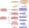 |
Fig. 1 Nemesis workflow. The parameter star_evol toggles stellar evolution on or off. Communication between codes is internally managed by AMUSE via channels. Orange boxes indicate simulation setup and termination, red boxes represent steps where work is offloaded to external codes, and blue boxes denote tasks returned to Python for manipulation of Nemesis-structured data. A movie showing Nemesis in action is available online. |
3.1 Validation 1: Direct N-body vs. Nemesis
The first set of simulations analyses the reliability of Nemesis (Section 4.2). To do so, we assume that the direct N-body integrator (Ph4) provides ground-truth results. That is, the greater the similarity between Ph4 and Nemesis, the more reliable Nemesis is deemed.
We use Ph4 to integrate both the parent and the children during Nemesis runs. We used the same integrator for the direct N-body run to facilitate comparisons between algorithms and to minimise computational load. We applied a softening of ϵ = 0.1 au in both schemes to further reduce computational load.
The cluster consists of N* = 2048 stars, distributed in a virialised Plummer (1911) sphere with half-mass radius rh = 0.5 pc. We drew stellar masses from a Kroupa (2001) mass distribution that ranged between 0.08–30 M⊙. We randomly sampled forty stars with masses between 0.5–2 M⊙ to host planetary systems (Nchd = 40). We integrate the cluster until 0.1 Myr, which was sufficient for systematic errors to become apparent. For Nemesis, we adopted a bridge time step of δtNem = 500 yr.
Planetary systems consist of one to six planets, whose masses and semi-major axes follow the oligarchic growth model (Kokubo & Ida 2002; Tremaine 2015), and 250 asteroids represented as test-particles (mast = 0 kg). The inner disc edge corresponds to a ten-year orbit, while the outer edge is given by ![Mathematical equation: $\[R_{\text {out}}=117 M_{\text {host}}^{0.45}\]$](/articles/aa/full_html/2026/05/aa58060-25/aa58060-25-eq6.png) au (Wilhelm et al. 2023). The asteroid disc has a Safronov–Toomre Q-parameter of Q = 1 (Safronov 1960; Toomre & Toomre 1972), and is distributed with surface density Σ ∝ r−3/2. We randomly oriented the systems along the ecliptic plane before any integration.
au (Wilhelm et al. 2023). The asteroid disc has a Safronov–Toomre Q-parameter of Q = 1 (Safronov 1960; Toomre & Toomre 1972), and is distributed with surface density Σ ∝ r−3/2. We randomly oriented the systems along the ecliptic plane before any integration.
We also performed an additional run in which Nemesis uses Huayno to integrate children, allowing a comparison of energy conservation. The internal time-step and softening parameter remain the same (η = 0.1 and ϵ = 0.1 au), but we ran the simulation to 1 Myr.
3.2 Validation 2: von Zeipel–Lidov–Kozai Effect
The second set of runs (Section 4.2) examined the von Zeipel–Lidov–Kozai effect (ZLK, von Zeipel 1910; Kozai 1962; Lidov 1962). The ZLK effect is a dynamical phenomenon in hierarchical triple systems, in which angular momentum is periodically exchanged between the inner and outer orbits when their mutual inclination exceeds a critical angle, ![Mathematical equation: $\[i_{\text {crit}}=\arctan~ \left(\sqrt{3 / 5}\right) \approx 39.2^{\circ}\]$](/articles/aa/full_html/2026/05/aa58060-25/aa58060-25-eq7.png) . Because the component of angular momentum parallel to the total angular momentum vector of the system,
. Because the component of angular momentum parallel to the total angular momentum vector of the system, ![Mathematical equation: $\[L_{z}= \sqrt{1-e^{2}} ~\cos~ i\]$](/articles/aa/full_html/2026/05/aa58060-25/aa58060-25-eq8.png) , and the semi-major axis (orbital energy) remains conserved, this interaction leads to coupled oscillations in the eccentricity and inclination of the inner orbit.
, and the semi-major axis (orbital energy) remains conserved, this interaction leads to coupled oscillations in the eccentricity and inclination of the inner orbit.
We setup the hierarchical triple identically to that in Figure 3 of Naoz et al. (2013a). Explicitly, the system contains an innerbinary composed of particles with masses M1 = 1 M⊙ and M2 = 1 MJup, orbiting with semi-major axis a = 6.0 au and eccentricity e = 10−3. The outer particle has mass M3 = 40 MJup and orbits the inner binary’s CoM with aout = 100 au and eout = 0.6. The initial inclination of the outer binary is iout = 65° relative to the inner orbital plane.
For each configuration, we conducted three tests. The first considers a regime with no parent-parent mergers, that is, Rpar = 0 au. The second considers a regime in which the child system never dissolves, that is, Rpar = 103 au > 2aout. The third considers a scenario with frequent parent-merging and child system dissolution events, sometimes both occurring within the same bridge time step, Rpar = 102 au. Unlike the first two configurations, which replicate results from a direct N-body code, the third configuration scrutinises the CoM approximation used to represent a child system within the parent integrator. It also tests Nemesis’s capability to handle parent-parent merging events and child system dissolution. We integrate systems for 10 Myr with a bridge time step of δtnem = 500 yr. For reference, this corresponds to half the orbital period of the outermost body.
In reality, when large eccentricities are reached (corresponding to inclination flips), tidal effects should be considered, and collisions may occur. In the present case, assuming a solar-radius object for our star-like particle, collisions occur when the inner binary reaches (1 − e) < 7.7 × 10⁻⁴. Although AMUSE supports collision detection and includes a symplectic integrator including tides to solve this (TIDYMESS, Boekholt & Correia 2023), we omit these to test Nemesis over longer times.
3.3 Computational scaling: Nemesis scaling Relations
The final set of runs investigated the computational scaling relations of Nemesis. We set up the simulated cluster environment similarly to that in Section 3.1. Planets followed the oligarchic model once more; however, we increased their number to eight per system, and asteroids are no longer considered.
We consider three cluster configurations: a massive, dense cluster with N* = 2048 and rh = 0.5 pc, a low-populated, sparse cluster with N* = 256 and rh = 0.5 pc, and a massive, sparse cluster with N* = 2048 and rh = 1 pc. The second and third configurations have equal densities. In all cases, we sampled the cluster from a Plummer distribution and set it initially in virial equilibrium. We integrate clusters until t = 0.1 Myr.
When analysing the dependence of computational resources on δtNem, we initially fixed the number of planetary systems to Nchd = 20 in all three configurations, while δtnem varied between 102–103 yr, in equal increments of 102 yr. When testing how the number of children influenced computational resources, we considered only the massive, dense cluster and fixed the bridge time step to δtNem = 103 yr. In this case, Nchd ranged from 20 to 60, spaced out in equal increments of ten. Although we used the same cluster realisation as the initial condition in all runs for the final test, varying Nchd, resulted in some runs having stars that hosted planetary systems and others did not.
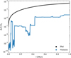 |
Fig. 2 Evolution of the simulation’s energy error in time. |
4 Results and discussion
4.1 Direct N-body vs. Nemesis
Figure 2 demonstrates Nemesis’s advantage in using a symplectic algorithm for its set of children, as its relative energy error remains bounded (see Figure A.4 of van Elteren et al. (2019) for another example). Jumps, however, still appear because the symplectic nature of Huayno hinders its ability to resolve close approaches.
In the purely direct N-body computation, Ph4 exhibits a steady drift in energy error, which, over longer timescales yields unreliable results, especially for rapidly evolving systems such as planetary systems. We used η = 0.1 for both runs; energy errors can be reduced by adjusting this parameter.
For the remainder of this section, the results correspond to the set of simulations in which Nemesis uses Ph4 for both the parent and child codes. Figs. 3 and 4 shows the cumulative distribution in semi-major axis, a, and eccentricity, e, for all bound asteroids at the end of the simulations.
We performed a Cramer–von Misses (Cramér 1928) test to assess statistical differences between results. This test compares distributions across the full range of values, unlike the Kolmogorov-Smirnov test, which probes only the region with the largest deviation. We find p-values of pa = 0.98 and pe = 0.93 for a and e, which implies that the distributions are indistinguishable.
Given the importance of the tail-end distribution in astronomy, since high-e orbits can induce system instabilities and/or trigger mergers/ejection events, we also applied a two-sample Anderson & Darling (1954) test. We find p-values of pa = 0.93 and pe = 0.50, allowing us to confidently reject the nullhypothesis that the two samples are drawn from different distributions. The large-scale cluster properties also show similar results, with both the distribution of stellar velocities and relative position having p = 1.
The similarity between distributions is further reflected in the residuals displayed in the upper panels of both plots. The residuals peak at max(Δy(e)) ≈ 0.012 and max(Δy(a)) ≈ 7 × 10⁻³, respectively. This corresponds to a ≲1.5% difference in population occupancy at any point in orbital-parameter space between the two algorithms. For the semi-major axis, Nemesis underestimates the semi-major axis of particles in the a ~ Rpar regime.
The residuals remain low and likely arise from statistical noise, a natural consequence of the chaotic nature of many-body dynamical systems. Nevertheless, Figure 4 shows that Nemesis performs worse when resolving the dynamical evolution of particles with semi-major axis a ~ Rpar. This discrepancy originates from the synchronisation between children and the global environment, which occurs at discrete time intervals (Section 2.2).
In Nemesis, correction kicks are applied only once every fixed bridge time step, δtNem. These bridge time steps are significantly larger than the internal integration time step δt used by gravitational solvers such as Ph4 (Equation (4)). While Ph4 accounts for the gravitational influence of all particles at every internal time step, child particles in Nemesis experience the external potential only at the bridge time steps. Between these bridge time steps, child particles only interact with other particles within the same child system.
Because it resolves external interactions at lower resolution and evaluates the potential when fly-by events are already relatively distant, Nemesis underestimates the effective potential. Child particles orbiting at a ~ Rpar are the most affected by this reduced resolution of the external potential.
Decoupling children systems from the global environment speeds computations (Section 4.3); however, this inevitably leads to a poorer representation of external perturbations. This trade-off is inherent to the method. As discussed in Section 2.2, setting δtnem → 0 yr produces results identical to a direct N-body code, but renders the algorithm highly inefficient.
Figure 5 illustrates the scenario more concretely. A planetary system with three planets (blue) and a host star (yellow) experiences a fly-by from an external star (pink). Although the perturber approaches the system, it never reaches a separation δrij ≤ Rpar,i + Rpar,j, where Rpar,j denotes the parent radius of the child system. As a result, using Nemesis, no parent merger is triggered during the parent integration and the gravitational interaction of the fly-by is treated exclusively in the parent code between relevant parents and during correction kicks between the perturber and the planetary system.
A direct N-body code accurately resolves this encounter by integrating the equations of motion at every internal time step (represented schematically by tracks on the fly-by trajectory). In contrast, under the fixed bridge implementation of Nemesis, where correction kicks are computed at increments of δtnem, close interactions are likely to be under-resolved or missed. Consequently, the algorithm predominantly samples the external potential when the perturber is already relatively distant, despite applying correction kicks. This effect is only significant in moderate encounters. If δrij ≤ Rpar,i + Rpar,j, the two systems merge and all relevant particles form a new child system whose internal dynamics are resolved using a dedicated symplectic integrator (Section 2.3).
In summary, Nemesis’s rigid bridge time-step implementation for synchronising local and global scales poorly resolves fly-by encounters too far away to trigger parent merging events, since the effective potential is likely to be computed only once the perturber is already far away. As a result, the effective external perturbation in Nemesis is weaker, making asteroids (or particles in general) less likely to scatter to large semi-major axes or high eccentricities. Figure 5 schematically illustrates this, showing the divergent paths of the planet under Nemesis (black arrow) and Ph4 (red arrow).
Although this has little impact on particles deep within the host potential, as reflected by the low residuals at small a in Figure 4, it becomes important near the boundary of children systems. This region contains particles that are least tightly bound to their host, and, therefore, most susceptible to the external environment. We are developing an adaptive bridge time-step scheme in Nemesis, with preliminary results using reinforcement learning showing promise (Saz Ulibarrena & Portegies Zwart 2025).
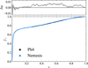 |
Fig. 3 Bottom: cumulative distribution function of asteroid eccentricities after tend = 0.1 Myr. Top: residuals in distributions between Nemesis and Ph4, computed as Δy(e) = (yNem(e) − yPh4(e)). |
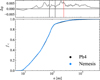 |
Fig. 4 Same as Figure 3 but for asteroid semi-major axis. The two vertical black lines in the upper panel represent the range in parent radius initially considered (0.5 ≤ Mpar [M⊙] ≤ 2.0) when using Equation (3) and A = 100. The red vertical line represents the linking length parameter, which flags children dissolution (Section 2.4) for a Mpar = 2 M⊙ parent host. |
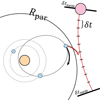 |
Fig. 5 Children on wide orbits are less as well resolved in Nemesis, was external interactions are applied via correction kicks every bridge time step (δtnem). The outer planet (blue) is diverted along the black trajectory. A direct N-body integrator computes interactions at every internal time-step (δt). With better resolution of the close encounter, the planet experiences a stronger gravitational effect and scatters outwards along the red path. |
4.2 von Zeipel–Lidov–Kozai Effect
Figure 6 shows the oscillation of the total inclination (itot = iout + iin) and the inner binaries’ eccentricity over time for all three runs. Runs using a test particle as the planetary mass object yield identical results and in both cases, Nemesis resolves the ZLK effect over secular times at an accuracy indistinguishable from a direct N-body integrator (the inlet in the lower panel highlights the extent to which Nemesis replicates results from a direct N-body integration). A relative energy error of ΔE = 3 × 10⁻¹² is found at the final step.
Theory estimates that the system considered here has a ZLK oscillation period of 0.913 Myr (Naoz et al. 2013b). The estimate uses a double-averaged Hamiltonian, and as such is an approximation. Additionally, they note that when the inner binary reaches large eccentricities (as the case here), the approximation can change by ‘orders of magnitude’. Even so, the value is near the oscillation timescale seen here (0.821 Myr). Even with the consistent splitting of the child system and merging of parent particles, the procedure doesn’t affect the dynamics, with a smooth evolution in the orbital parameters being observed. The result also highlights the validity of representing children with a CoM parent in the parent code.
The capability to capture the ZLK effect is important for resolving secular timescales for dynamical systems. For instance, in planetary systems, the ZLK effect has been proposed to create hot Jupiters (Holman & Wiegert 1999; Mustill et al. 2017) and has been considered for the evolution of asteroids (Naoz et al. 2012; Fernández et al. 2004). Meanwhile, in the galactic nuclei, the ZLK effect will drive black hole-black hole mergers or hyper velocity stars (Naoz et al. 2013b; Fragione & Leigh 2018; Zevin et al. 2019; Arca Sedda et al. 2021). For an overview see Naoz (2016).
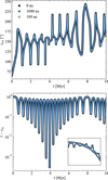 |
Fig. 6 Total inclination of the triple system (top) and inner binary eccentricity (bottom) over time. The system consists of an inner binary (M1 = 1 M⊙, M2 = 40 MJup) perturbed by an outer binary of mass M = 40 MJup. The inset shows the oscillation in (1 − ein) for the first 0.12 Myr. One cycle lasts 0.821 Myr. The y axis corresponds to Δ(1 − e) = 3 × 10⁻³, illustrating the accuracy with which Nemesis captures ZLK cycles. |
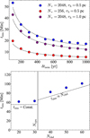 |
Fig. 7 Top: Nemesis bridge time step δtnem versus computation time for an identical cluster containing 20 subsystems. Blue points correspond to a cluster with density ρ ~ 103 M⊙ pc−3, while red and purple points ρ ~ 102 M⊙ pc−3. Dashed lines indicate curves with exponent α = −0.5. Bottom: number of children Nchd versus time taken to simulate an identical cluster to 100 kyr, tsim. |
4.3 Nemesis scaling relations
4.3.1 Bridge time step
The top panel of Figure 7 shows how Nemesis performs as the bridge time step, δtnem, changes. This time step defines when children and parents synchronise and communicate their respective gravitational potentials with one another.
We fit the relation ![Mathematical equation: $\[t_{\text {sim}} \propto \delta t_{\text {nem}}^{\alpha}\]$](/articles/aa/full_html/2026/05/aa58060-25/aa58060-25-eq9.png) with power-laws, finding α = −0.52 ± 0.02 for the blue points, α = −0.58 ± 0.02 for the red points and α = −0.56 ± 0.01 for the purple points. However, the curves all consider α = −0.5 as this value provides reasonable fits. The slope depends on what dominates the calculation. For large N*, the gravitational code dominates run time, whereas for low N*, algorithmic overhead plays a larger role. This is reflected in the slightly shallower slopes in the high-density, massive cluster runs, where algorithmic overhead now plays a smaller role.
with power-laws, finding α = −0.52 ± 0.02 for the blue points, α = −0.58 ± 0.02 for the red points and α = −0.56 ± 0.01 for the purple points. However, the curves all consider α = −0.5 as this value provides reasonable fits. The slope depends on what dominates the calculation. For large N*, the gravitational code dominates run time, whereas for low N*, algorithmic overhead plays a larger role. This is reflected in the slightly shallower slopes in the high-density, massive cluster runs, where algorithmic overhead now plays a smaller role.
There is no unique optimum time step. Users should conduct test runs to determine the optimal parameter. Ultimately there is a trade-off between computational resources saved from increasing δtnem and associated loss of accuracy. Ideally, Nemesis would use an adaptive algorithm. For example, as a cluster evolves and expands, long-range perturbations weaken, allowing δtnem to relax to larger values. As discussed in Section 4.1, an adaptive time step scheme has not yet been implemented but is planned for future work.
Wall-clock time taken to simulate Nchd systems till 0.1 Myr.
4.3.2 Number of children
The bottom panel of Figure 7 shows how Nchd affects the computation time. Here, we execute NCPU = 32 worker processes using MPI.
As expected, while Nchd < NCPU, the run-time is approximately constant. However, when Nchd > NCPU, the scaling becomes linear (the best fit gives a power-law α = 0.978 ± 0.002). The linear trend represents a worst-case scenario, in which all children require roughly the same computational time to integrate, and results from child codes hibernating until resources (linear in NCPU) become available. In theory, given the hardware of certain supercomputers, this scaling implies that simulating globular clusters in which each star hosts a planetary system is now attainable. As a final comparison between a direct N-body method and Nemesis, Table 1 compares the time needed to simulate identical systems to 0.1 Myr.
4.4 Parent radius
Although we did not directly test it, the choice of Rpar also affects performance and reliability. If Rpar is too large, children are more likely to include multiple particles of comparable mass, which reduces the accuracy of the CoM approximation. Decreasing δtnem can mitigate errors, but at the cost of increased computation time (Figure 7) and without fully correcting the underlying issue.
Since the strength of Nemesis lies in the decoupling of small-scale systems from the large-scale environment, it is generally preferable to keep Rpar small; the value should be tested for optimal performance. There are several reasons for choosing small Rpar (at the cost of larger δtnem):
Centre-of-mass approximation: smaller Rpar makes the CoM approximation more successful, since it is less likely that any system has two massive particles with a similar mass ratio, q ≡ mi/mj. In the situation where a system has the mass ratio between its two most massive particles of q → 1, the omission of correction kicks between particles of two distinct child systems starts to break down. Similarly, when Rpar is too large, wide orbits shift the CoM and decrease accuracy.
Avoiding bottlenecks from tight orbits: the problem of directly integrating small-scale systems in large-scale environments (i.e., planetary systems in clusters) is the need to suppress the drift in energy errors to capture secular effects. This can be achieved with symplectic codes. However, with their shared time step scheme, the tightest orbits induce a bottleneck in the integration. With Nemesis, as long as Rpar exceeds the tightest orbit of a typical system, tight orbits are decoupled from the global integration, removing the bottleneck for the parent integration while allowing accurate integration of the internal dynamics. This scheme is indifferent to how much Rpar exceeds the scale of the tightest orbit.
Parent particle merging events: the collision handler in AMUSE internally checks at every time step whether two particles collide. Since cluster codes utilise an adaptive time step, that scales with the particle’s free-fall time (see Equation (4)), all collision events within the parent are detected unless the timestep is exceedingly small.
Throughout the testing, a radius coefficient A = 100 sufficed (see Equation (3)). This was tested for environments with densities between ρ ~ (102–104) M⊙ pc−3 but may change depending on the initial cluster parameters, i.e., the initial virality or compactness of systems.
However, Section 4.1 illustrates that particles with a semi-major axis a ~ Rpar are poorly resolved. As such, given the points listed above, it may be worthwhile to use a lower value. While this does not fix the underlying problem as child particles will still exist with a ~ Rpar, particles with smaller semi-major axes are better protected from the external environment, and deviations should be less substantial.
A conservative Rpar implies that wide systems, i.e., wide planets or Oort Cloud-like environments (Öpik 1932; Oort 1950), fall back to the parent code. While this does not resolve the local dynamics as successfully, the long secular timescales of wide orbits partly compensate for the loss in accuracy. Moreover, such systems are inherently fragile, and external tides or encounters with field particles are likely to strip them before secular effects become significant. There is a delicate balance between δtnem and Rpar, and it remains for future work to find a logical and adaptable way to balance the two for a given system, keeping in mind the computation time and the accuracy of the results.
5 Conclusions
The multi-scale, multi-physics nature of astronomy complicates computational astrophysics. This work formally introduces an updated and optimised version of the Nemesis hybrid code, which has previously been used to simulate planetary systems in an Orion-like cluster (van Elteren et al. 2019).
After describing the motivation and theory behind the scheme in Section 2, we ran a suite of simulations to test its performance. The first test examined asteroids within the evolution of a star cluster. Comparison with a direct N-body code, shows the algorithms produce statistically indistinguishable final orbital parameters for asteroids. When tracking the energy error over longer periods of time, Nemesis successfully suppresses energy drift when using symplectic codes. This feature is essential for simulating systems over secular timescales. The success in modelling secular effects is highlighted by the second set of tests, which demonstrates the ability to reproduce the ZLK oscillations in hierarchical triples.
Finally, we conducted two scaling tests. The first examined how the wall-clock time scales with the bridge time step, δtNem. While smaller δtnem lowers integration error, it increases algorithmic overhead; the wall-clock time scales as ![Mathematical equation: $\[t_{\text {sim}} \propto 1 / \sqrt{\delta t_{\text {nem}}}\]$](/articles/aa/full_html/2026/05/aa58060-25/aa58060-25-eq10.png) . Users should therefore perform trial runs before production runs to determine the optimal δtnem since this may depend on the environment. Indeed, the virial state, density and/or binary fraction may all play a role. In the second scaling test, we examined how the number of subsystems present, Nchd, influences the wall-clock time. The runtime remains constant while Nchd remains below the number of available CPUs. Beyond this point, computational cost scales at worst linearly. This behaviour emphasises the highly parallelised nature of Nemesis and its ability to integrate environments hosting numerous subsystems.
. Users should therefore perform trial runs before production runs to determine the optimal δtnem since this may depend on the environment. Indeed, the virial state, density and/or binary fraction may all play a role. In the second scaling test, we examined how the number of subsystems present, Nchd, influences the wall-clock time. The runtime remains constant while Nchd remains below the number of available CPUs. Beyond this point, computational cost scales at worst linearly. This behaviour emphasises the highly parallelised nature of Nemesis and its ability to integrate environments hosting numerous subsystems.
Software is never finished, but even in its current form, Nemesis provides researchers with a practical means to tackle multi-scale and multi-physics problems. Given the flexibility of the algorithm and the AMUSE environment hosting numerous codes in the domain of hydrodynamics, gravity, radiative transport, chemistry and stellar evolution codes, creative solutions to complex problems are now attainable.
Data availability
Movie associated to Fig. 1 is available at https://www.aanda.org
Acknowledgements
We thank the referee for providing nice suggestions which improved the quality and clarity of this paper. Analysis was made using the opensource Python packages NumPy (Harris et al. 2020) and Matplotlib (Hunter 2007).
References
- Aarseth, S. J., & Zare, K. 1974, Celest. Mech., 10, 185 [NASA ADS] [CrossRef] [Google Scholar]
- Ahmad, A., & Cohen, L. 1973, J. Computat. Phys., 12, 389 [NASA ADS] [CrossRef] [Google Scholar]
- Anderson, T. W., & Darling, D. A. 1954, J. Am. Statist. Assoc., 49, 765 [CrossRef] [Google Scholar]
- Arca Sedda, M., Amaro Seoane, P., & Chen, X. 2021, A&A, 652, A54 [NASA ADS] [CrossRef] [EDP Sciences] [Google Scholar]
- Bailer-Jones, C. A. L. 2011, MNRAS, 416, 1163 [Google Scholar]
- Barnes, J., & Hut, P. 1986, Nature, 324, 446 [NASA ADS] [CrossRef] [Google Scholar]
- Boekholt, T., & Portegies Zwart, S. 2015, Computat. Astrophys. Cosmol., 2, 2 [NASA ADS] [CrossRef] [Google Scholar]
- Boekholt, T. C. N., & Correia, A. C. M. 2023, MNRAS, 522, 2885 [Google Scholar]
- Boekholt, T. C. N., Moerman, A., & Portegies Zwart, S. F. 2021, Phys. Rev. D, 104, 083020 [CrossRef] [Google Scholar]
- Bovy, J. 2015, ApJS, 216, 29 [NASA ADS] [CrossRef] [Google Scholar]
- Cai, M. X., Kouwenhoven, M. B. N., Portegies Zwart, S. F., & Spurzem, R. 2017, MNRAS, 470, 4337 [Google Scholar]
- Cohn, H. 1979, ApJ, 234, 1036 [NASA ADS] [CrossRef] [Google Scholar]
- Cramér, H. 1928, Scand. Actuar. J., 1928, 13 [CrossRef] [Google Scholar]
- Davis, M., Hut, P., & Muller, R. A. 1984, Nature, 308, 715 [Google Scholar]
- Dejonghe, H., & Hut, P. 1986, in Lecture Notes in Physics, 267, eds. P. Hut, & S. L. W. McMillan, 212 [Google Scholar]
- Fernández, J. A., Gallardo, T., & Brunini, A. 2004, Icarus, 172, 372 [CrossRef] [Google Scholar]
- Fragione, G., & Leigh, N. 2018, MNRAS, 480, 5160 [Google Scholar]
- Fujii, M., Iwasawa, M., Funato, Y., & Makino, J. 2007, PASJ, 59, 1095 [NASA ADS] [Google Scholar]
- Giersz, M. 1998, MNRAS, 298, 1239 [NASA ADS] [CrossRef] [Google Scholar]
- Gropp, W., Lusk, E., Doss, N., & Skjellum, A. 1996, Parallel Comput., 22, 789 [Google Scholar]
- Harris, C. R., Millman, K. J., van der Walt, S. J., et al. 2020, Nature, 585, 357 [NASA ADS] [CrossRef] [Google Scholar]
- Heggie, D. C. 2003, in IAU Symposium, 208, Astrophysical Supercomputing using Particle Simulations, eds. J. Makino, & P. Hut, 81 [Google Scholar]
- Hénon, M. H. 1971, Ap&SS, 14, 151 [Google Scholar]
- Hernquist, L. 1990, ApJ, 356, 359 [Google Scholar]
- Hills, J. G. 1980, ApJ, 235, 986 [NASA ADS] [CrossRef] [Google Scholar]
- Holman, M. J., & Wiegert, P. A. 1999, AJ, 117, 621 [Google Scholar]
- Huang, S., Portegies Zwart, S., & Wilhelm, M. J. C. 2024, A&A, 689, A338 [NASA ADS] [CrossRef] [EDP Sciences] [Google Scholar]
- Hunter, J. D. 2007, Comput. Sci. Eng., 9, 90 [NASA ADS] [CrossRef] [Google Scholar]
- Iwasawa, M., Portegies Zwart, S., & Makino, J. 2015, Computat. Astrophys. Cosmol., 2, 6 [NASA ADS] [CrossRef] [Google Scholar]
- Kirkpatrick, J. D., Cushing, M. C., Gelino, C. R., et al. 2011, ApJS, 197, 19 [NASA ADS] [CrossRef] [Google Scholar]
- Kokubo, E., & Ida, S. 2002, ApJ, 581, 666 [Google Scholar]
- Kozai, Y. 1962, AJ, 67, 591 [Google Scholar]
- Kroupa, P. 2001, MNRAS, 322, 231 [NASA ADS] [CrossRef] [Google Scholar]
- Lada, C. J., & Lada, E. A. 2003, ARA&A, 41, 57 [Google Scholar]
- Lada, C. J., Lombardi, M., & Alves, J. F. 2010, ApJ, 724, 687 [Google Scholar]
- Lidov, M. L. 1962, Planet. Space Sci., 9, 719 [Google Scholar]
- Makino, J., & Aarseth, S. J. 1992, PASJ, 44, 141 [NASA ADS] [Google Scholar]
- Mannerkoski, M., Rawlings, A., Johansson, P. H., et al. 2023, MNRAS, 524, 4062 [Google Scholar]
- McMillan, S., Portegies Zwart, S., van Elteren, A., & Whitehead, A. 2012, in Astronomical Society of the Pacific Conference Series, 453, Advances in Computational Astrophysics: Methods, Tools, and Outcome, eds. R. Capuzzo-Dolcetta, M. Limongi, & A. Tornambè, 129 [Google Scholar]
- Miyamoto, M., & Nagai, R. 1975, PASJ, 27, 533 [NASA ADS] [Google Scholar]
- Mustill, A. J., Davies, M. B., & Johansen, A. 2017, MNRAS, 468, 3000 [Google Scholar]
- Naoz, S. 2016, ARA&A, 54, 441 [Google Scholar]
- Naoz, S., Farr, W. M., & Rasio, F. A. 2012, ApJ, 754, L36 [NASA ADS] [CrossRef] [Google Scholar]
- Naoz, S., Farr, W. M., Lithwick, Y., Rasio, F. A., & Teyssandier, J. 2013a, MNRAS, 431, 2155 [NASA ADS] [CrossRef] [Google Scholar]
- Naoz, S., Kocsis, B., Loeb, A., & Yunes, N. 2013b, ApJ, 773, 187 [NASA ADS] [CrossRef] [Google Scholar]
- Navarro, J. F., Frenk, C. S., & White, S. D. M. 1997, ApJ, 490, 493 [Google Scholar]
- Nelemans, G., Yungelson, L. R., Portegies Zwart, S. F., & Verbunt, F. 2001, A&A, 365, 491 [NASA ADS] [CrossRef] [EDP Sciences] [Google Scholar]
- Noether, E. 1918, Nachr. D. König. Gesellsch. D. Wiss. Zu Göttingen, 235 [Google Scholar]
- Oort, J. H. 1950, Bull. Astron. Inst. Netherlands, 11, 91 [NASA ADS] [Google Scholar]
- Öpik, E. 1932, Proc. Am. Acad. Arts Sci., 67, 169 [Google Scholar]
- Paxton, B., Bildsten, L., Dotter, A., et al. 2011, ApJS, 192, 3 [Google Scholar]
- Pelupessy, F. I., Jänes, J., & Portegies Zwart, S. 2012, New A, 17, 711 [NASA ADS] [CrossRef] [Google Scholar]
- Pelupessy, F. I., van Elteren, A., de Vries, N., et al. 2013, A&A, 557, A84 [NASA ADS] [CrossRef] [EDP Sciences] [Google Scholar]
- Plummer, H. C. 1911, MNRAS, 71, 460 [Google Scholar]
- Poincaré, H. 1891, Bull. Astron. Ser. I, 8, 12 [Google Scholar]
- Poincaré, H. 1892, Les méthodes nouvelles de la mécanique céleste (Paris: Gauthier-Villars et fils) [Google Scholar]
- Portegies Zwart, S. F., & Verbunt, F. 1996, A&A, 309, 179 [NASA ADS] [Google Scholar]
- Portegies Zwart, S. F., & Yungelson, L. R. 1998, A&A, 332, 173 [NASA ADS] [Google Scholar]
- Portegies Zwart, S., & McMillan, S. 2018, Astrophysical Recipes; The Art of AMUSE (IOP Publishing) [Google Scholar]
- Portegies Zwart, S., McMillan, S., Harfst, S., et al. 2009, New A, 14, 369 [NASA ADS] [CrossRef] [Google Scholar]
- Portegies Zwart, S. F., McMillan, S. L. W., & Gieles, M. 2010, ARA&A, 48, 431 [Google Scholar]
- Rantala, A., Pihajoki, P., Johansson, P. H., et al. 2017, ApJ, 840, 53 [Google Scholar]
- Rein, H., & Liu, S. F. 2012, A&A, 537, A128 [NASA ADS] [CrossRef] [EDP Sciences] [Google Scholar]
- Safronov, V. S. 1960, Ann. Astrophys., 23, 979 [NASA ADS] [Google Scholar]
- Saz Ulibarrena, V., & Portegies Zwart, S. 2025, Commun. Nonlinear Sci. Numer. Simul., 145, 108723 [Google Scholar]
- Spitzer, Jr., L., & Hart, M. H. 1971, ApJ, 164, 399 [NASA ADS] [CrossRef] [Google Scholar]
- Spurzem, R., Giersz, M., Takahashi, K., & Ernst, A. 2005, MNRAS, 364, 948 [Google Scholar]
- Stiefel, E., & Kustaanheimo, P. 1965, J. Reine Angew. Math., 218, 204 [Google Scholar]
- Toomre, A., & Toomre, J. 1972, ApJ, 178, 623 [Google Scholar]
- Toonen, S., Nelemans, G., & Portegies Zwart, S. 2012, A&A, 546, A70 [NASA ADS] [CrossRef] [EDP Sciences] [Google Scholar]
- Tremaine, S. 2015, ApJ, 807, 157 [Google Scholar]
- van Elteren, A., Pelupessy, I., & Portegies Zwart, S. 2014, Philos. Trans. Roy. Soc. London Ser. A, 372, 20130385 [Google Scholar]
- van Elteren, A., Portegies Zwart, S., Pelupessy, I., Cai, M. X., & McMillan, S. L. W. 2019, A&A, 624, A120 [NASA ADS] [CrossRef] [EDP Sciences] [Google Scholar]
- Verlet, L. 1967, Phys. Rev., 159, 98 [CrossRef] [Google Scholar]
- von Zeipel, H. 1910, Astron. Nachr., 183, 345 [Google Scholar]
- Wang, L., Iwasawa, M., Nitadori, K., & Makino, J. 2020, MNRAS, 497, 536 [NASA ADS] [CrossRef] [Google Scholar]
- Whitmire, D. P., & Jackson, A. A. 1984, Nature, 308, 713 [Google Scholar]
- Wilhelm, M. J. C., Portegies Zwart, S., Cournoyer-Cloutier, C., et al. 2023, MNRAS, 520, 5331 [NASA ADS] [CrossRef] [Google Scholar]
- Winter, A. J., Haworth, T. J., Coleman, G. A. L., & Nayakshin, S. 2022, MNRAS, 515, 4287 [NASA ADS] [CrossRef] [Google Scholar]
- Wisdom, J., & Holman, M. 1991, AJ, 102, 1528 [Google Scholar]
- Zevin, M., Samsing, J., Rodriguez, C., Haster, C.-J., & Ramirez-Ruiz, E. 2019, ApJ, 871, 91 [NASA ADS] [CrossRef] [Google Scholar]
All Tables
All Figures
|
Fig. 1 Nemesis workflow. The parameter star_evol toggles stellar evolution on or off. Communication between codes is internally managed by AMUSE via channels. Orange boxes indicate simulation setup and termination, red boxes represent steps where work is offloaded to external codes, and blue boxes denote tasks returned to Python for manipulation of Nemesis-structured data. A movie showing Nemesis in action is available online. |
| In the text | |
|
Fig. 2 Evolution of the simulation’s energy error in time. |
| In the text | |
|
Fig. 3 Bottom: cumulative distribution function of asteroid eccentricities after tend = 0.1 Myr. Top: residuals in distributions between Nemesis and Ph4, computed as Δy(e) = (yNem(e) − yPh4(e)). |
| In the text | |
|
Fig. 4 Same as Figure 3 but for asteroid semi-major axis. The two vertical black lines in the upper panel represent the range in parent radius initially considered (0.5 ≤ Mpar [M⊙] ≤ 2.0) when using Equation (3) and A = 100. The red vertical line represents the linking length parameter, which flags children dissolution (Section 2.4) for a Mpar = 2 M⊙ parent host. |
| In the text | |
|
Fig. 5 Children on wide orbits are less as well resolved in Nemesis, was external interactions are applied via correction kicks every bridge time step (δtnem). The outer planet (blue) is diverted along the black trajectory. A direct N-body integrator computes interactions at every internal time-step (δt). With better resolution of the close encounter, the planet experiences a stronger gravitational effect and scatters outwards along the red path. |
| In the text | |
|
Fig. 6 Total inclination of the triple system (top) and inner binary eccentricity (bottom) over time. The system consists of an inner binary (M1 = 1 M⊙, M2 = 40 MJup) perturbed by an outer binary of mass M = 40 MJup. The inset shows the oscillation in (1 − ein) for the first 0.12 Myr. One cycle lasts 0.821 Myr. The y axis corresponds to Δ(1 − e) = 3 × 10⁻³, illustrating the accuracy with which Nemesis captures ZLK cycles. |
| In the text | |
|
Fig. 7 Top: Nemesis bridge time step δtnem versus computation time for an identical cluster containing 20 subsystems. Blue points correspond to a cluster with density ρ ~ 103 M⊙ pc−3, while red and purple points ρ ~ 102 M⊙ pc−3. Dashed lines indicate curves with exponent α = −0.5. Bottom: number of children Nchd versus time taken to simulate an identical cluster to 100 kyr, tsim. |
| In the text | |
Current usage metrics show cumulative count of Article Views (full-text article views including HTML views, PDF and ePub downloads, according to the available data) and Abstracts Views on Vision4Press platform.
Data correspond to usage on the plateform after 2015. The current usage metrics is available 48-96 hours after online publication and is updated daily on week days.
Initial download of the metrics may take a while.