| Issue |
A&A
Volume 708, April 2026
|
|
|---|---|---|
| Article Number | A273 | |
| Number of page(s) | 9 | |
| Section | The Sun and the Heliosphere | |
| DOI | https://doi.org/10.1051/0004-6361/202558826 | |
| Published online | 14 April 2026 | |
Linking long-term switchback variability at 1 au to solar-surface mechanisms: A 27-year statistical study
1
State Key Laboratory of Solar Activity and Space Weather, National Space Science Center, Chinese Academy of Sciences, Beijing, 100190, China
2
University of Chinese Academy of Sciences, Beijing, 100049, China
★ Corresponding author: This email address is being protected from spambots. You need JavaScript enabled to view it.
Received:
30
December
2025
Accepted:
14
March
2026
Abstract
Context. Switchbacks–transient, large-angle deflections of the interplanetary magnetic field–pervade the solar wind, yet their origin remains disputed. Current ex situ theories, notably coronal jets and interchange reconnection, are typically tested on day-scale intervals.
Aims. We aim to establish a connection between switchbacks and ex situ theories on solar-cycle timescales.
Methods. We exploited 27 years of continuous in situ measurements from ACE, Wind, and STEREO-A/B at 1 au, complemented by synoptic remote-sensing data from SDO, to examine the solar-cycle modulation of switchback occurrence and to test whether ex situ scenarios (coronal jets and interchange reconnection) play a dominant role in such long-term modulation.
Results. The switchback occurrence rate correlates strongly with Alfvénicity (cc = 0.70 ± 0.04) and shows no solar-maximum preference (independent of the sunspot number, cc = 0.13 ± 0.05). Coronal jets affect switchbacks only indirectly via modulation of the solar wind speed. Multi-spacecraft consensus confirms that a stable, Alfvénicity-dependent process governs switchback variability, rather than episodic surface drivers. In addition, these results are robust to the deflection threshold of switchbacks. These findings impose quantitative constraints on theories of solar-wind turbulence and the transport of magnetic energy from the Sun to interplanetary space.
Key words: Sun: heliosphere / Sun: magnetic fields / solar wind
© The Authors 2026
 Open Access article, published by EDP Sciences, under the terms of the Creative Commons Attribution License (https://creativecommons.org/licenses/by/4.0), which permits unrestricted use, distribution, and reproduction in any medium, provided the original work is properly cited.
This article is published in open access under the Subscribe to Open model. This email address is being protected from spambots. You need JavaScript enabled to view it. to support open access publication.
1. Introduction
Switchbacks are transient structures characterized by large-angle deflections of the interplanetary magnetic field caused by the localized folding of solar wind field lines. They are ubiquitously observed in the near-sun solar wind (Horbury et al. 2018; Bale et al. 2019; Kasper et al. 2019). Their formation mechanisms remain contested, broadly categorized into two groups: (1) ex situ generation via solar surface processes – coronal jets (Sterling & Moore 2020) and interchange reconnection (Fisk & Kasper 2020; Zank et al. 2020; Liang et al. 2021; Drake et al. 2021; He et al. 2021). Specifically, Bale et al. (2023) emphasized that interchange reconnection generates patches of switchbacks rather than individual structures, whereas Shi et al. (2022) interpreted these patches as temporal features in the evolving solar wind. Alternatively, (2) in situ production through solar wind dynamics involves wave expansion and turbulence (Squire et al. 2020; Shoda et al. 2021; Mallet et al. 2021; Squire et al. 2022; Johnston et al. 2022; Matteini et al. 2024; Bowen et al. 2025; Sioulas et al. 2025), velocity shear (Ruffolo et al. 2020; Toth et al. 2023), and footpoint motion (Schwadron & McComas 2021).
Due to findings that switchback occurrence rates and deflection magnitudes gradually decrease near the Sun (Pecora et al. 2022; Jagarlamudi et al. 2023), and that small-deflection magnetic switchback events typically predominate below the Alfvén critical region (Liu et al. 2023) – although large-deflection events can occur under specific conditions – the “ex situ” generation mechanism has been revised into a two-step scenario (Akhavan-Tafti & Soni 2024). Specifically, these mechanisms do not directly reproduce full-reversal switchbacks. Instead, they propose a two-step process: solar events only generate the initial seeds, which may later evolve into full reversal switchbacks through wave expansion.
Recent attempts made to link switchbacks to solar-surface origins combined near-Sun in situ observations (e.g., PSP and SolO) with remote sensing data (e.g., SDO) (de Pablos et al. 2022; Raouafi et al. 2023). For example, Kumar et al. (2023), Hou et al. (2024a,b) employed the potential field source surface (PFSS) model to link switchbacks with coronal jets (or jetlets) during several distinct day-scale time windows. However, determining the magnetic connectivity within short-term windows faces significant uncertainties. As shown in Badman et al. (2023), the choice of boundary conditions can lead to significant instability in magnetic connectivity for certain encounters, such as Encounter 4. In the same vein, Bizien et al. (2025) demonstrated that inferred source regions are highly sensitive to both source-surface height selection and propagation speed assumptions.
Switchbacks have also been observed by spacecraft such as Wind and ACE operating near 1 au, and even by the more distant Ulysses (Yamauchi et al. 2004; Gosling et al. 2009; Matteini et al. 2014; Borovsky 2016). Bourouaine et al. (2022) reported that the Wind spacecraft observed intervals of solar wind at 1 au that were strikingly similar to those measured by PSP within 0.3 au, both characterized by a high abundance of switchbacks. Statistical analyses further indicate that the average occurrence rate of switchbacks near 1 au is comparable to, and potentially even higher than, that in regions closer to the Sun (Macneil et al. 2020; Tenerani et al. 2021; Pecora et al. 2022).
In this study, we employed long-term observations spanning over two solar cycles from the ACE and Wind spacecrafts operating near 1 au, together with complementary measurements from STEREO-A and STEREO-B to investigate the temporal evolution of the switchback occurrence rate. We further combined these in situ measurements with long-term remote-sensing data from SDO to explore their connection to solar surface mechanisms.
Section 2 describes the dataset and methodology, including the identification of switchbacks and the detection of Alfvénic fluctuations. Our results are presented in Section 3, with a discussion provided in Section 4. Our conclusions are summarized in Section 5.
2. Datasets and methodology
2.1. Spacecraft data and solar activity indices
We analyzed in situ measurements from the following four spacecraft operating near 1 au:
-
ACE: Magnetic field data from MAG (Smith et al. 1998) supplemented by OMNI2 plasma parameters (King & Papitashvili 2005) (1998-01-01 to 2025-07-22);
-
Wind: Magnetic field data from MFI (Lepping et al. 1995) and plasma data from 3DP (Lin et al. 1995) (1994-11-13 to 2025-08-19; selected for XGSE > 20RE);
-
STEREO-A: Magnetic field data from IMPACT (Acuña et al. 2008) and plasma data from PLASTIC (Galvin et al. 2008) (2007-01-01 to 2025-06-30);
-
STEREO-B: Same instruments as STEREO-A (2007-05-01 to 2014-09-27).
All magnetic field data were interpolated to a 3-second resolution. Following Li et al. (2025), we selected continuous segments > 6 hours with a maximum gap duration ≤120 s.
Solar activity indices include:
-
Daily sunspot numbers (Clette et al. 2014) (WDC-SILSO, Royal Observatory of Belgium, Brussels);
-
Coronal holes (CHs) and coronal brightenings (CBs) identified using data from the Atmospheric Imaging Assembly (AIA; Lemen et al. 2012) instrument and Helioseismic and Magnetic Imager (HMI; Scherrer et al. 2012) magnetograms on board the Solar Dynamics Observatory (SDO; Pesnell et al. 2012).
2.2. Diagnosis of switchbacks
Switchbacks were identified using a multistep procedure from our previous work (Li et al. 2025), which employed the normalized deflection angle z proposed by Dudok de Wit et al. (2020):
![Mathematical equation: $$ \begin{aligned} z(t) = \frac{1}{2} \left[1-cos\theta (t)\right] , \end{aligned} $$](/articles/aa/full_html/2026/04/aa58826-25/aa58826-25-eq1.gif) (1)
(1)
where θ denotes the angle between the local and the background magnetic field.
The identification procedure consists of the following five steps:
-
Potential event detection: We identified events with normalized deflection angle z > 0.15, where the background magnetic field for calculating z was obtained using a 1-hour sliding average.
-
Adjacent events merging: We combined adjacent events if the separation Δt was less than the duration of the longer switchbacks Tl.
-
Single-point event exclusion: We discarded events consisting of only a single data point to ensure robust identification.
-
Compressibility screening: We excluded events with
 over the ±Δt window, where σ|B| is the standard deviation of magnetic field intensity and ⟨|B|⟩ is the averaged magnetic field intensity.
 -
HCS exclusion: We removed potential heliospheric current sheet (HCS) crossings using the method proposed by Pecora et al. (2022).
The parameters employed in this study – namely, the z = 0.15 threshold, the 1-hour background window, and the compressibility criterion – represent operational choices required for statistical quantification, despite their inherent arbitrariness and limitations.
First, as demonstrated by Dudok de Wit et al. (2020), switchbacks are self-similar structures lacking a characteristic duration or deflection angle. Consequently, the z = 0.15 threshold is indeed one of many possible choices in a continuous distribution. Nevertheless, this threshold effectively captures statistically significant deflections in practice, and sensitivity tests using alternative thresholds (z = 0.10 and z = 0.25) are presented in the results section.
Second, the 1-hour background window may exclude large-amplitude switchbacks with periods exceeding one hour – given that typical Alfvén-wave periods at 1 au range from 103 to 105 s (Bruno & Carbone 2013; Huang et al. 2025) –potentially underestimating their contribution to the total fluctuation energy (Matteini et al. 2014). However, according to Dudok de Wit et al. (2020), the durations of switchbacks follow a power-law distribution. Therefore, this methodological choice may not significantly affect the statistical characteristics of our results. Similarly, sensitivity tests using alternative time windows (2-hour and 3-hour) are presented in the results section.
Third, the compressibility criterion, while similarly arbitrary, is necessary to exclude intervals where significant magnetic field strength variations could lead to misidentification of switchbacks. The choice of threshold was inspired by Tenerani et al. (2021).
Finally, given that switchbacks are recognized as continuous Alfvénic fluctuations – rather than isolated discrete structures (Badman et al. 2026) – providing information on their temporal occupancy offers a more informative perspective than event counts alone. Accordingly, we supplement our analysis with an examination of temporal occupancy in the discussion section.
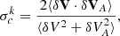
2.3. Alfvénicity quantification
Solar wind Alfvénicity was quantified using the Err parameter proposed by Li et al. (2016). When Err approaches 0, the solar wind exhibits maximal Alfvénicity:
 (2)
(2)
where ℳi includes ||γc|−1|, ||γcx|−1|, ||γcy|−1|, ||γcz|−1|, |σδV/σδVA − 1|, and |σδVx/σδVAx − 1|. Here, γc denotes the plasma velocity-Alfvén velocity correlation coefficient, and σ represents the standard deviation.
Using data from the Wind spacecraft, we calculated Errk in five logarithmically spaced frequency bands (i.e., 100–160 s, 160–250 s, 250–400 s, 400–630 s, and 630–1000 s). The mean Alfvénicity index  per segment was computed as
 (3)
(3)
To facilitate direct comparison with previous studies that commonly employ cross helicity as a measure of Alfvénicity, we also computed the normalized cross helicity (σc) following the same procedure as for Err. For each of the same five frequency bands, we calculated σck as
 (4)
(4)
where δV and δVA are the fluctuations in velocity and Alfvén velocity within the specified frequency band and the angle brackets denote averages over time windows set to 1.5 times the upper period of the corresponding frequency band (the same intervals used for Errk). The mean normalized cross helicity  per segment was then computed as
 (5)
(5)
2.4. Diagnosis of high-speed streams
We applied a previously developed machine classification method (Li et al. 2020) to identify high-speed streams (HSSs) using hourly averaged solar wind data from the OMNI database1 starting from May 19, 2010. This method achieves an accuracy of over 95% in detecting HSSs. We selected events with solar wind speeds exceeding 500 km/s that persisted for at least 24 hours and were flagged as HSSs. Time intervals separated by less than two hours were merged into a single event. Furthermore, we utilized event lists from Richardson & Cane (2010), Chi et al. (2016) to exclude contaminating coronal mass ejection (CME) events.
We then calculated the average solar wind speed VHSS during each HSS interval (marked by start time tstart and end time tend) to estimate its transit time ΔT = R/VHSS from the Sun to the satellite, with R representing 0.99 au. Subsequently, we identified CHs and searched for CBs within the time range from tstart − ΔT to tend − ΔT.
2.5. Automated coronal hole detection
Coronal holes are recognized as sources of fast solar wind (Krieger et al. 1973). In our study, CHs are automatically identified using the multi-thermal emission recognition algorithm CHIMERA (Garton et al. 2018). This method relies on emission intensity from three extreme ultraviolet wavelengths (171, 193, and 211 Å) supplemented by magnetograms. The automated detection of CHs is processed on an hourly basis. To enhance data continuity, we consolidated the computational results obtained every three hours. Furthermore, all identified boundaries were uniformly extended by 24 arc seconds to ensure complete coverage of the adjacent regions surrounding the CHs.
2.6. Automated coronal brightening detection
We utilized CBs as a proxy for jet occurrence in this study. These brightenings, which correspond to the jet base, are a direct manifestation of the underlying interchange magnetic reconnection process (Sterling et al. 2015). Since the visibility of the jet structure is not guaranteed due to insufficient brightness contrast and unfavorable observation angles, tracking these more persistent and easily detectable brightenings provides a more robust indicator of jet activity.
We adapted an automated detection methodology, based on the approach of Hou et al. (2024a) for CBs, to identify CBs within the mainly CH region located at the solar disk center. The field of view for this analysis is a rectangular region in heliocentric coordinates, spanning from −323 to 608 arc seconds in solar-X and from −473 to 473 arc seconds in solar-Y. The process involves analyzing SDO/AIA 193 Å images by normalizing the intensity by exposure time, computing 10-minute cadence differential images and applying a brightness increase threshold of 35% to isolate significant brightening events.
3. Results
3.1. Relationship with the solar activity cycle
Figure 1 presents the temporal evolution of OR (switchbacks per hour) derived from 27-day sliding averages (with a 1-day step size sliding window). For clarity, the left panel shows only data points from nonoverlapping windows (1/27 of the total). Given that switchbacks are, by definition, Alfvénic structures (Badman et al. 2026), their occurrence rate is inherently influenced by the Alfvénicity of the solar wind (Li et al. 2025); here, we again employ the  parameter as a reference metric.
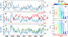 |
Fig. 1. Temporal evolution and parameter correlations of the switchback occurrence rate. Left: 27-day sliding averages of the switchback occurrence rate (OR, blue) and sunspot number (SSN, gray) in panel (a), along with two Alfvénicity indices– |


Figure 1(a)-(b) shows that OR varies between 0.69 and 4.86–a sevenfold range–indicating significant month-to-month and interannual variations. Overall, OR exhibits a strong negative correlation with  (cc = −0.75) and a positive correlation with Alfvénicity; however, we find no systematic correlation with sunspot number SSN (cc = 0.15).
Panel (c) serves as a counterpart to panel (b) in Fig. 1, showing the relationship between  and OR. The absolute correlation coefficient between
  and OR differs by only 0.01 from that obtained with
  , indicating that the two Alfvénicity metrics exhibit nearly identical relationships with OR. Remarkably, the correlation coefficient between
  and
and  itself reaches -0.996, demonstrating an almost linear relationship. This confirms that the two parameters are essentially interchangeable for quantifying solar wind Alfvénicity in this study.
Figure 1(d)-(e) further deconstruct the temporal relationship by presenting the average occurrence rate OR under different  and SSN conditions. In this visualization, OR clearly peaks where the solar wind exhibits the highest Alfvénicity (corresponding to the lowest
  ), rather than in regions of highest SSN. Moreover, within fixed
  bins, higher SSN corresponds to slightly reduced OR. Notably, normalizing the sunspot number within each solar cycle (Figure 1(e)) does not lead to any substantial changes in the overall distribution pattern or the revealed relationships.
Table 1 further quantifies the correlation coefficients of the above relationships under different identification thresholds, background windows, and normalization schemes. As the deflection angle increases, the absolute correlation coefficient between the occurrence rate and  decreases but remains relatively high. In comparison, the SSN correlation shows a similar trend yet remains consistently low. Regarding the background window, as the window length increases, the absolute correlation coefficients with both
  and SSN increase again. When the normalization method is switched from per unit time to per unit distance, the absolute correlation coefficients with
  generally decrease, with a maximum reduction of only 0.04. The changes in correlation with SSN are even smaller, with a maximum variation of merely 0.02. These results indicate that the aforementioned differences do not affect the key characteristics: the occurrence rates remain highly correlated with solar wind Alfvénicity but show no correlation with sunspot number.
Correlation coefficients with  and SSN.
Table 1 indicates that the unit-distance normalization–intended to correct for biases from the varying relative speed between the spacecraft and the solar wind–is insufficient to eliminate the velocity-dependent effects rooted in solar wind Alfvénicity differences (Li et al. 2025). Consequently, the systematic bias inherent in using averaged values as reference values for a specific heliocentric distance persist.
Figure 2 demonstrates the influence of VSW. Panel (a) further reveals the differences under the four solar cycle phases (max, min, ascending, and descending). Although all four curves exhibit a broadly similar upward trend, two systematic deviations are observed. First, the OR values for the ascending and maximum phases are slightly lower in the high VSW regime. This is likely attributed to a higher occurrence rate of CMEs during these periods; this difference is eliminated after excluding CME events following the aforementioned list (Richardson & Cane 2010; Chi et al. 2016). Second, the OR for the minimum phase exhibits relative lag in its growth rate at low solar wind speeds, forming a slight relative depression. We postulate that this is due to systematically lower solar wind Alfvénicity during this period (D’Amicis et al. 2021), particularly in the slow wind. This depression disappears when constraining solar wind Alfvénicity. The same mechanism also accounts for the relationship between the OR and SSN seen in Fig. 1(d)-(e), by which the solar wind at solar minimum requires higher velocity to reach similar levels of Err.
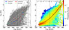 |
Fig. 2. Dependence of OR on solar wind speed (VSW). Panel (a): Scatter plot of OR vs. VSW using a 2-day sliding window (1-hour cadence), with overplotted averages and standard errors for solar maximum (red; 24 months before to 6 months after solar maxima in 2001-11-01, 2014-04-01, and 2024-08-01), solar minimum (blue; same window around solar minima in 1996-08-01, 2008-12-01, and 2019-12-01), as well as for the intermediate ascending and descending phases (light cyan and light lime). Panel (b): Conditional probability distributions of OR for different VSW ranges. The smoothing curve was fitted exclusively to the primary, contiguous high-density region (probability density > 0.02), whose outline is indicated by the white or gray contour in the figure. Minor, isolated regions were excluded from the fit. |
Figure 2(b) reveals a distinct, concentrated distribution region. Although a linear fit applied to the portion with VSW between 500 and 750 km/s also shows high consistency, the region is overall better suited for a quadratic fit. This fitted curve can be used for correction: the correlation between OR and Err after additive and multiplicative corrections is significantly reduced to −0.39 and −0.35, respectively, while the correlation with SSN remains low (0.07 and 0.10).
3.2. Relationship with coronal brightening activity
While our previous studies established switchback concentration within HSS – a type of high-Alfvénicity solar wind – their occurrence rate during these periods still exhibits substantial variability. To explore the origin of this variability, we investigate its potential link to the frequent occurrence of jets within the source CHs.
Using the method described previously, we identify 141 HSS events with clear CH associations. The screening procedure involved two criteria:
-
Primary CH stability: For each timestamp in the interval, we identified the largest CH (primary CH) and restricted our analysis to periods when its area exceeds 80% of its median value over the interval.
-
Primary CH dominance: Within this constrained time range, the primary CH must cover over 5% of the total field of view and constitute more than 95% of the total CH area within the field of view for more than 50% of the time.
Figure 3 shows the relationship between NCB and the switchback occurrence rate before and after correction (denoted as OR and OR*, respectively) during HSS intervals. Overall, the occurrence rate shows no clear relationship with NCB (correlation coefficients are 0.03 and –0.13, respectively). Since the variation in background brightness can introduce bias (Madjarska 2019) and failure to account for this effect may lead to misleading conclusions, supplementary analyses of subsets characterized by high (red, encompassing periods of solar maximum) and low (blue, encompassing periods of solar minimum) brightness are included.
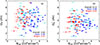 |
Fig. 3. Panel (a): Relationship between OR and the number of brightening points per unit area within the primary CH NCB during HSS periods. The horizontal error bars indicate the ratio of the standard deviation to the mean. Panel (b): Same as (a), but with OR replaced by the corrected occurrence rate OR*, where OR* = OR ⋅ f(550)/f(VHSS), f is the fitting function from Fig. 2(b), and VHSS is the average solar wind speed during the HSS interval. |
After separating by brightness, Figure 3(a) shows that within the two subsets exhibiting clear horizontal offsets, the correlation coefficient between OR and NCB increases notably compared to the overall case (cc = 0.30 and 0.21 for the low-and high-brightness groups, respectively). However, it remains at a low level (not exceeding 0.3). Figure 3(b) shows that after correction, the two quantities become virtually uncorrelated (cc = 0.00 and 0.02). Finally, we note that the main conclusions of this analysis are not sensitive to the specific choice of thresholds in the event selection process.
3.3. Consistency across multiple spacecraft observations
To verify the reliability of the observations, we compare in Figure 4 the results from different spacecraft within the two previously used time windows. Figure 4(a) compares OR from four near-ecliptic but different longitude spacecraft near 1 au. ACE and Wind (located in similar areas) exhibit near-identical trends (cc = 0.98) in the occurrence rate. STEREO-A/B observations remain consistent with ACE (cc = 0.75 and 0.72), despite temporally varying longitudinal separations.
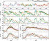 |
Fig. 4. Multi-spacecraft comparison at 1 au. Panel (a): Temporal variations of OR (using the same 27-day sliding window in Fig. 1) observed by ACE (blue), Wind (red), STEREO-A (orange), and STEREO-B (green). Panels (b)-(c): VSW and OR (using the same 2-day sliding window in Fig. 2) for the time intervals corresponding to the shaded regions in panel (a). The dashed black lines mark the onset times of the HSS observed by ACE, defined as the moments when VSW exceeds 500 km/s (accurate to the hour). Panels (d)-(g): Time-series superposition of the two sets of distinct 27-day repeating HSS intervals from (b)-(c), aligned at their respective onset times (t = 0). |
Figure 4(b)-(g) provides detailed zoom-ins on the shaded intervals from panel (a). Panel (b) reveals the presence of two distinct, 27-day repeating HSSs (with durations of about 4 and 8 days, respectively), each observed three times by ACE, STEREO-A, and STEREO-B, as documented by Borovsky (2016). The nine individual observations of these two streams are displayed in panels (d, f) and (e, g), respectively, where the time axes have been aligned relative to the onset of the streams, defined as the moment the speed first exceeds 500 km/s. After alignment, OR exhibits a common evolutionary pattern across both the HSS and its surrounding regions, with the average occurrence levels during the HSS periods also being highly comparable.
4. Discussion
The open-closed boundary (OCB), which separates open and closed magnetic field lines, is considered an ideal (but not exclusive) site for interchange reconnection (Liu et al. 2023). Wilkins et al. (2025) found that the fraction of the Sun’s open flux originating near the OCB, which is much higher at solar maximum (near 100%) than at minimum (near 10%), strongly correlates with the sunspot number. Based on this correlation, they speculated that if interchange reconnection (Fisk & Kasper 2020; Zank et al. 2020; Drake et al. 2021; Bale et al. 2023) is the dominant mechanism, OR should be significantly enhanced during solar maximum.
The data in Section 3.1 provide an opportunity to test this prediction. However, not only did the time series fail to reveal a significant positive correlation (with a correlation coefficient of only 0.2), but OR during solar maximum also showed no pronounced elevation, even when constraining the analysis to periods of similar Err or VSW.
Beyond its application for correction, the result from Figure 2(b) leads us to prefer the VSW-OR relationship to represent the switchback distribution within a specified heliocentric distance range. In the future, combining such curves obtained at different heliocentric distances (e.g., from PSP and SolO) will likely help elucidate the switchback evolution in solar winds of different speeds (or types).
To date, there has been no statistical study on the relationship between switchbacks and jet activity (indirectly represented by CBs in this study) in the context of coronal jet generation mechanisms (Sterling & Moore 2020). This work aims to fill that gap by utilizing long-term observations at 1 au.
However, the correlation between NCB and OR (0.30 and 0.21 for the two subsets, respectively) is weak. Moreover, the correlation nearly vanishes when considering OR* (0.00 and 0.02), which attempts to remove the influence of VHSS. This indicates that jets have a relatively weak direct influence on OR and their primary contribution lies in indirectly affecting OR through driving HSS (VHSS).
The high consistency of the multi-spacecraft results in Figure 4 not only enhances the reliability of our findings but also suggests that switchback generation and evolution are likely driven by a stable process, as evidenced by solar wind from the same source region maintaining similar OR levels over an extended period. This stability effectively broadens the usable time window for multi-spacecraft studies at different heliocentric distances, thereby relaxing the requirement for strict temporal alignment between observations.
Finally, note that we examined results under different deflection thresholds and background windows (Table 1) throughout this study. Varying these parameters only changes the total number of identified events – with lower z thresholds or longer background windows naturally selecting more events – without affecting any of our conclusions. Notably, the pairwise correlation coefficients between occurrence rates obtained under the five different parameter combinations exceed 0.95 under the 27-day sliding window.
Beyond the occurrence rate, we also examined the temporal occupancy of switchbacks – defined as the total duration of switchbacks per unit time (minutes per hour). We find that replacing the occurrence rate with temporal occupancy does not alter any of our main conclusions. For example, under the five parameter combinations listed in Table 1, replacing the occurrence rate with temporal occupancy yields correlation coefficients with  of −0.79, −0.75, −0.69, −0.70, and −0.71, respectively, and with SSN of 0.22, 0.16, 0.08, 0.13, and 0.16. These values are qualitatively identical to those obtained with the occurrence rate.
Figure 5 shows a linear relationship between the switchback occurrence rate and temporal occupancy under the 27-day sliding window, with correlation coefficients no less than 0.95 for all parameter combinations. Namely, under the 2-day sliding window, the distribution becomes more scattered, yet the correlation coefficients remain above 0.90. Accordingly, we provide linear fits forced through the origin, with slopes of 2.17, 1.73, 1.25, 1.77, and 2.10 minutes per event, in the same order as presented in Table 1. These values are nearly identical to those obtained by directly averaging event durations. These slopes facilitate conversion between the two metrics and enable comparison with studies that report switchback prevalence in terms of temporal occupancy.
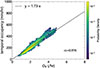 |
Fig. 5. Joint distribution of the switchback occurrence rate and temporal occupancy, using the same 27-day sliding window in Fig. 1. |
5. Summary
This study presents the first long-term analysis of the switchback occurrence rate using 27 years of observations at 1 au. Our main findings include the following.
-
The absence of positive solar cycle dependence: The switchback occurrence rate shows a negligible correlation with sunspot number and does not peak during solar maximum.
-
The indirect role of coronal jets: Coronal jets exhibit only an indirect influence on the switchback rate, primarily by driving high-speed solar wind streams.
-
Consistency across spacecraft: High cross-correlation in long-term and short-term observations among ACE, Wind, STEREO-A, and STEREO-B observations indicates that the generation and evolution of switchbacks are dominated by a stable process.
This work represents an initial effort to connect long-term observations at 1 au with solar surface mechanisms. Our future work will investigate the long-term behavior of jetlets and their relationship to coronal jets, incorporate CH morphological characteristics into the analysis, and evaluate various surface mechanisms as potential triggers for other switchback models.
Acknowledgments
The authors thank the NASA CDAWEB (https://cdaweb.gsfc.nasa.gov/) for providing the ACE, Wind, and STEREO-A/B data, the OMNI database (https://omniweb.gsfc.nasa.gov/) for providing the solar wind data, and the Joint Science Operations Center (http://jsoc.stanford.edu/) for providing the SDO data. This work was supported by the National Key R&D Program of China (2025YFE0202500), NNSFC grants (42374198, 42188101), and the project of Civil Aerospace “14th Five-Year Plan” Preliminary Research in Space Science (D010302, D010202). H. Li was also supported by the China-Brazil Joint Laboratory for Space Weather grant (119GJHZ2024027MI).
References
- Acuña, M., Curtis, D., Scheifele, J., et al. 2008, Space Sci. Rev., 136, 203 [Google Scholar]
- Akhavan-Tafti, M., & Soni, S. 2024, ApJ, 970, L26 [Google Scholar]
- Badman, S. T., Riley, P., Jones, S. I., et al. 2023, J. Geophys. Res. Space Phys., 128, e2023JA031359 [Google Scholar]
- Badman, S. T., Fargette, N., Matteini, L., et al. 2026, Space Sci. Rev., 222, 14 [Google Scholar]
- Bale, S., Badman, S., Bonnell, J., et al. 2019, Nature, 576, 237 [Google Scholar]
- Bale, S., Drake, J., McManus, M., et al. 2023, Nature, 618, 252 [Google Scholar]
- Bizien, N., Froment, C., Madjarska, M. S., de Wit, T. D., & Velli, M. 2025, A&A, 694, A181 [Google Scholar]
- Borovsky, J. E. 2016, J. Geophys. Res. Space Phys., 121, 5055 [Google Scholar]
- Bourouaine, S., Perez, J. C., Raouafi, N. E., et al. 2022, ApJ, 932, L13 [Google Scholar]
- Bowen, T. A., Mallet, A., Dunn, C. I., et al. 2025, A&A, 700, A51 [Google Scholar]
- Bruno, R., & Carbone, V. 2013, Liv. Rev. Sol. Phys., 10, 2 [Google Scholar]
- Chi, Y., Shen, C., Wang, Y., et al. 2016, Sol. Phys., 291, 2419 [Google Scholar]
- Clette, F., Svalgaard, L., Vaquero, J. M., & Cliver, E. W. 2014, Space Sci. Rev., 186, 35 [CrossRef] [Google Scholar]
- D’Amicis, R., Alielden, K., Perrone, D., et al. 2021, A&A, 654, A111 [NASA ADS] [CrossRef] [EDP Sciences] [Google Scholar]
- de Pablos, D., Samanta, T., Badman, S. T., et al. 2022, Sol. Phys., 297, 90 [NASA ADS] [CrossRef] [Google Scholar]
- Drake, J., Agapitov, O., Swisdak, M., et al. 2021, A&A, 650, A2 [NASA ADS] [CrossRef] [EDP Sciences] [Google Scholar]
- Dudok de Wit, T., Krasnoselskikh, V. V., Bale, S. D., et al. 2020, ApJS, 246, 39 [Google Scholar]
- Fisk, L., & Kasper, J. 2020, ApJS, 894, L4 [Google Scholar]
- Galvin, A. B., Kistler, L. M., Popecki, M. A., et al. 2008, Space Sci. Rev., 136, 437 [Google Scholar]
- Garton, T. M., Gallagher, P. T., & Murray, S. A. 2018, J. Space Weather Space Clim., 8, A02 [NASA ADS] [CrossRef] [EDP Sciences] [Google Scholar]
- Gosling, J., McComas, D., Roberts, D., & Skoug, R. M. 2009, ApJ, 695, L213 [Google Scholar]
- He, J., Zhu, X., Yang, L., et al. 2021, ApJL, 913, L14 [Google Scholar]
- Horbury, T., Matteini, L., & Stansby, D. 2018, MNRAS, 478, 1980 [Google Scholar]
- Hou, C., He, J., Duan, D., et al. 2024a, Nat. Astron., 8, 1246 [Google Scholar]
- Hou, C., Rouillard, A. P., He, J., et al. 2024b, ApJ, 968, L28 [NASA ADS] [CrossRef] [Google Scholar]
- Huang, Z., Velli, M., Chandran, B., et al. 2025, ApJ, 990, L34 [Google Scholar]
- Jagarlamudi, V. K., Raouafi, N., Bourouaine, S., et al. 2023, ApJ, 950, L7 [Google Scholar]
- Johnston, Z., Squire, J., Mallet, A., & Meyrand, R. 2022, Phys. Plasmas, 29 [Google Scholar]
- Kasper, J. C., Bale, S. D., Belcher, J. W., et al. 2019, Nature, 576, 228 [Google Scholar]
- King, J., & Papitashvili, N. 2005, J. Geophys. Res. Space Phys., 110 [Google Scholar]
- Krieger, A., Timothy, A., & Roelof, E. 1973, Sol. Phys., 29, 505 [NASA ADS] [CrossRef] [Google Scholar]
- Kumar, P., Karpen, J. T., Uritsky, V. M., et al. 2023, ApJ, 951, L15 [CrossRef] [Google Scholar]
- Lemen, J. R., Title, A. M., Akin, D. J., et al. 2012, Sol. Phys., 275, 17 [Google Scholar]
- Lepping, R., Acũna, M., Burlaga, L., et al. 1995, Space Sci. Rev., 71, 207 [NASA ADS] [CrossRef] [Google Scholar]
- Li, H., Wang, C., Chao, J., & Hsieh, W. 2016, J. Geophys. Res. Space Phys., 121, 42 [Google Scholar]
- Li, H., Wang, C., Tu, C., & Xu, F. 2020, Earth Space Sci., 7, e2019EA000997 [Google Scholar]
- Li, H., Dai, F., Wang, C., Jiang, W., & Li, H. 2025, ApJ, 984, L4 [Google Scholar]
- Liang, H., Zank, G. P., Nakanotani, M., & Zhao, L.-L. 2021, ApJ, 917, 110 [Google Scholar]
- Lin, R., Anderson, K., Ashford, S., et al. 1995, Space Sci. Rev., 71, 125 [Google Scholar]
- Liu, Y. D., Ran, H., Hu, H., & Bale, S. D. 2023, ApJ, 944, 116 [NASA ADS] [CrossRef] [Google Scholar]
- Macneil, A. R., Owens, M. J., Wicks, R. T., et al. 2020, MNRAS, 494, 3642 [Google Scholar]
- Madjarska, M. S. 2019, Liv. Rev. Sol. Phys., 16, 2 [Google Scholar]
- Mallet, A., Squire, J., Chandran, B. D., Bowen, T., & Bale, S. D. 2021, ApJ, 918, 62 [NASA ADS] [CrossRef] [Google Scholar]
- Matteini, L., Horbury, T. S., Neugebauer, M., & Goldstein, B. E. 2014, Geophys. Res. Lett., 41, 259 [Google Scholar]
- Matteini, L., Tenerani, A., Landi, S., et al. 2024, Phys. Plasmas, 31 [Google Scholar]
- Pecora, F., Matthaeus, W. H., Primavera, L., et al. 2022, ApJ, 929, L10 [NASA ADS] [CrossRef] [Google Scholar]
- Pesnell, W. D., Thompson, B., & Chamberlin, P. 2012, Sol. Phys., 275, 3 [Google Scholar]
- Raouafi, N. E., Stenborg, G., Seaton, D. B., et al. 2023, ApJ, 945, 28 [NASA ADS] [CrossRef] [Google Scholar]
- Richardson, I. G., & Cane, H. V. 2010, Sol. Phys., 264, 189 [NASA ADS] [CrossRef] [Google Scholar]
- Ruffolo, D., Matthaeus, W. H., Chhiber, R., et al. 2020, ApJ, 902, 94 [Google Scholar]
- Scherrer, P. H., Schou, J., Bush, R., et al. 2012, Sol. Phys., 275, 207 [Google Scholar]
- Schwadron, N., & McComas, D. 2021, ApJ, 909, 95 [NASA ADS] [CrossRef] [Google Scholar]
- Shi, C., Panasenco, O., Velli, M., et al. 2022, ApJ, 934, 152 [CrossRef] [Google Scholar]
- Shoda, M., Chandran, B. D., & Cranmer, S. R. 2021, ApJ, 915, 52 [CrossRef] [Google Scholar]
- Sioulas, N., Velli, M., Shi, C., et al. 2025, arXiv e-prints [arXiv:2510.10106] [Google Scholar]
- Smith, C. W., L’Heureux, J., Ness, N. F., et al. 1998, Space Sci. Rev., 86, 613 [Google Scholar]
- Squire, J., Chandran, B. D., & Meyrand, R. 2020, ApJ, 891, L2 [NASA ADS] [CrossRef] [Google Scholar]
- Squire, J., Johnston, Z., Mallet, A., & Meyrand, R. 2022, Phys. Plasmas, 29 [Google Scholar]
- Sterling, A. C., & Moore, R. L. 2020, ApJ, 896, L18 [Google Scholar]
- Sterling, A. C., Moore, R. L., Falconer, D. A., & Adams, M. 2015, Nature, 523, 437 [NASA ADS] [CrossRef] [Google Scholar]
- Tenerani, A., Sioulas, N., Matteini, L., et al. 2021, ApJ, 919, L31 [NASA ADS] [CrossRef] [Google Scholar]
- Toth, G., Velli, M., & van der Holst, B. 2023, ApJ, 957, 95 [Google Scholar]
- Wilkins, C. P., Pontin, D. I., Yeates, A. R., et al. 2025, ApJ, 985, 190 [Google Scholar]
- Yamauchi, Y., Suess, S. T., Steinberg, J. T., & Sakurai, T. 2004, J. Geophys. Res. Space Phys., 109 [Google Scholar]
- Zank, G., Nakanotani, M., Zhao, L.-L., Adhikari, L., & Kasper, J. 2020, ApJ, 903, 1 [NASA ADS] [CrossRef] [Google Scholar]
Appendix A: Switchback identification and occurrence rate calculation
This section presents an example of identifying switchbacks and calculating their occurrence rate. In Figure A.1, the start and end times of the five identified switchback events are marked by black dashed lines. Based on this, the temporal occurrence rate for this specific hour is determined to be 5 events per hour. Combining this with the average solar wind speed of 602 km/s during that hour, the occurrence rate can be converted to a spatial scale, yielding approximately 2.3 events per million km.
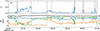 |
Fig. A.1. Example of a switchback interval. (a) Normalized deflection angle, z; (b) Magnetic field components in RTN coordinates. |
All Tables
All Figures
|
Fig. 1. Temporal evolution and parameter correlations of the switchback occurrence rate. Left: 27-day sliding averages of the switchback occurrence rate (OR, blue) and sunspot number (SSN, gray) in panel (a), along with two Alfvénicity indices– |
| In the text | |
|
Fig. 2. Dependence of OR on solar wind speed (VSW). Panel (a): Scatter plot of OR vs. VSW using a 2-day sliding window (1-hour cadence), with overplotted averages and standard errors for solar maximum (red; 24 months before to 6 months after solar maxima in 2001-11-01, 2014-04-01, and 2024-08-01), solar minimum (blue; same window around solar minima in 1996-08-01, 2008-12-01, and 2019-12-01), as well as for the intermediate ascending and descending phases (light cyan and light lime). Panel (b): Conditional probability distributions of OR for different VSW ranges. The smoothing curve was fitted exclusively to the primary, contiguous high-density region (probability density > 0.02), whose outline is indicated by the white or gray contour in the figure. Minor, isolated regions were excluded from the fit. |
| In the text | |
|
Fig. 3. Panel (a): Relationship between OR and the number of brightening points per unit area within the primary CH NCB during HSS periods. The horizontal error bars indicate the ratio of the standard deviation to the mean. Panel (b): Same as (a), but with OR replaced by the corrected occurrence rate OR*, where OR* = OR ⋅ f(550)/f(VHSS), f is the fitting function from Fig. 2(b), and VHSS is the average solar wind speed during the HSS interval. |
| In the text | |
|
Fig. 4. Multi-spacecraft comparison at 1 au. Panel (a): Temporal variations of OR (using the same 27-day sliding window in Fig. 1) observed by ACE (blue), Wind (red), STEREO-A (orange), and STEREO-B (green). Panels (b)-(c): VSW and OR (using the same 2-day sliding window in Fig. 2) for the time intervals corresponding to the shaded regions in panel (a). The dashed black lines mark the onset times of the HSS observed by ACE, defined as the moments when VSW exceeds 500 km/s (accurate to the hour). Panels (d)-(g): Time-series superposition of the two sets of distinct 27-day repeating HSS intervals from (b)-(c), aligned at their respective onset times (t = 0). |
| In the text | |
|
Fig. 5. Joint distribution of the switchback occurrence rate and temporal occupancy, using the same 27-day sliding window in Fig. 1. |
| In the text | |
|
Fig. A.1. Example of a switchback interval. (a) Normalized deflection angle, z; (b) Magnetic field components in RTN coordinates. |
| In the text | |
Current usage metrics show cumulative count of Article Views (full-text article views including HTML views, PDF and ePub downloads, according to the available data) and Abstracts Views on Vision4Press platform.
Data correspond to usage on the plateform after 2015. The current usage metrics is available 48-96 hours after online publication and is updated daily on week days.
Initial download of the metrics may take a while.