| Issue |
A&A
Volume 708, April 2026
|
|
|---|---|---|
| Article Number | A348 | |
| Number of page(s) | 9 | |
| Section | Numerical methods and codes | |
| DOI | https://doi.org/10.1051/0004-6361/202558532 | |
| Published online | 23 April 2026 | |
AI application to artificial satellite identification in CHEOPS data
Scanning the CHEOPS image archive with a neural network
1
Safran,
171 Bd de Valmy,
92700
Colombes,
France
2
CFisUC, Departamento de Física, Universidade de Coimbra,
Coimbra,
3004-516,
Portugal
3
Laboratory of Astrophysics, EPFL,
Chemin Pegasi 51,
1290
Versoix,
Switzerland
4
Observatoire Astronomique de l’Université de Genève,
Chemin Pegasi 51,
1290
Versoix,
Switzerland
5
European Space Agency (ESA), European Space Astronomy Centre (ESAC), Camino Bajo del Castillo s/n,
28692
Villanueva de la Cañada, Madrid,
Spain
★ Corresponding author: This email address is being protected from spambots. You need JavaScript enabled to view it.
Received:
11
December
2025
Accepted:
20
March
2026
Abstract
Context. The rapid proliferation of artificial satellites poses a growing challenge to astronomical observations, calling for robust methods to flag and mitigate their impact on scientific data quality. Modern astronomical surveys, including space-based missions such as CHEOPS, generate vast data volumes, where the manual identification of these contaminants is unfeasible. Artificial intelligence (AI) has emerged as an essential tool for efficiently processing these large datasets, enabling the automated flagging of transient features to preserve the scientific value of the data.
Aims. We developed and validated a computationally efficient AI algorithm, based on the MobileNetV2 architecture, to detect satellite trails in CHEOPS images. We benchmarked this novel method against traditional linear feature detection algorithms to assess trade-offs in terms of sensitivity and speed.
Methods. We trained a binary classifier using an iteratively enhanced dataset, incorporating “hard-negative” examples (e.g., cosmic rays, stray light, Earth limb proximity) to minimize the false-positive rate. The final model was applied to the entire CHEOPS archive of 1.8 million images (up to June 2025). The detections were cross-matched with the Space-Track database to identify objects, enabling a detailed analysis of their physical parameters and magnitude evolution over time.
Results. The AI model achieved 99.2% accuracy on the test set and identified 12 223 satellite trails in the archive (0.68% of all images), more than double the yield of non-AI methods, demonstrating superior sensitivity to faint trails. The post-processing identification matched these trails to 5565 distinct objects. While our photometric analysis from 2020 to 2025 shows a constant average standard magnitude (13.4 ± 1.7) for the aggregate detection set, an analysis against launch dates reveals a trend of newer objects appearing brighter.
Conclusions. AI-based methods provide a powerful and sensitive tool for detecting satellite trails in space-based observatories. However, they do require careful training to generalize against complex image artifacts.
Key words: methods: data analysis / astronomical databases: miscellaneous
© The Authors 2026
 Open Access article, published by EDP Sciences, under the terms of the Creative Commons Attribution License (https://creativecommons.org/licenses/by/4.0), which permits unrestricted use, distribution, and reproduction in any medium, provided the original work is properly cited.
This article is published in open access under the Subscribe to Open model. This email address is being protected from spambots. You need JavaScript enabled to view it. to support open access publication.
1 Introduction
Characterizing ExOPlanet Satellite (CHEOPS, Benz et al. 2021) is the first small (S-class) mission within the European Space Agency’s (ESA) space science Cosmic Vision program, developed as a partnership between Switzerland and ESA. Successfully launched on December 18, 2019, into a 700 km sunsynchronous orbit, CHEOPS is the first space mission dedicated to searching for exoplanet transits by performing ultra-high precision photometry on bright stars that are already known to host planets. Its primary objective is to improve existing radii measurements or determine new accurate radii for planets whose masses have been estimated from ground-based surveys. This allows for a detailed characterization of planetary bulk properties to constrain formation and evolution models. The high-precision photometry also enables CHEOPS to measure exoplanet phase curves and search for other features, such as exo-moons or rings. By identifying and characterizing transiting exoplanets with high potential, CHEOPS provides prime targets for future instruments dedicated to the spectroscopic study of exoplanetary atmospheres.
The rapid expansion of artificial satellites in Earth’s orbit, while essential for global connectivity, services and our everyday life, introduces a new and growing challenge for astronomy. As these objects traverse the night sky, their reflective surfaces can reflect sunlight, which appears as bright streaks in sensitive telescopic images. These trails can complicate astronomical observations, potentially contaminating scientific data or obscuring faint signals from distant celestial objects, creating a complex new variable for researchers to manage.
The proliferation of satellite constellations has spurred critical research into mitigating their impact on astronomical images. Current strategies are multi-faceted. Tyson et al. (2020) laid down a foundational work by investigating a suite of options and sensor-level algorithm-based corrections for the Rubin Observatory Legacy Survey of Space and Time (LSST). On the operational front, and for this same observatory, Hu et al. (2022) argued that an upgraded observatory scheduler can effectively avoid satellite-dense regions, presenting a direct trade-off between reduced streaks and total observing time. For contaminated data, post-processing is key. Hasan et al. (2022) studied trail masking, highlighting the challenge of faint residuals that can still be present in the final data. Finally, for spectroscopic observations where spatial information is often lacking, Hainaut & Moehler (2024) concluded that statistical rejection via multiple sub-exposures remains the most effective mitigation strategy.
Efforts to mitigate interference from satellite constellations also include strategies focused on intrinsic satellite design. A primary goal is minimizing apparent brightness (increasing the apparent magnitude) by reducing satellite reflectance. The International Astronomical Union’s (IAU) Centre for the Protection of the Dark and Quiet Sky (CPS)1 facilitates this approach by actively engaging satellite operators to adopt low-reflectivity designs, aiming to minimize the impact on astronomy (Boley et al. 2025).
A precedent for quantifying the impact of artificial satellites on space-based observatories was set by Kruk et al. (2023). This work provided one of the first quantitative measurements of human-made objects imaged from a low Earth orbit (LEO), analyzing Hubble Space Telescope’s archive from 2002 to 2021, establishing a baseline and demonstrating that this fraction is increasing over time.
Regarding the CHEOPS mission, Billot et al. (2024) also demonstrated a growing trend in space-based satellite detections in CHEOPS images in the interval from March 2020 until May 2023 (see examples in Figure 1). Over this period, the authors observed an overall increase in the detection rate of trails caused by resident space objects. This steep rise was most significant in the high-density shell corresponding to LEO, consistent with the increase of satellites launched into this orbit during that same time period.
On a more operational note, space-based monitoring of human-made objects provides significant operational advantages. It enables the visual characterization of smaller-scale objects, allowing for a more comprehensive assessment of the orbital debris population and paving the way for future removal missions (Liou et al. 2010; Dhinakaran et al. 2025). Furthermore, this capability is essential for facilitating rendezvous and proximity operations (RPO), where one spacecraft maneuvers to approach a target object. These operations support both cooperative applications (e.g., maintenance, repair, and overhaul) and non-cooperative scenarios, such as active debris removal or defense-related applications (Jenkins 2024).
The integration of artificial intelligence (AI) in astronomy and astrophysics is a rapidly growing trend driven by necessity. Modern and upcoming surveys, such as the Vera C. Rubin Observatory LSST and the Square Kilometer Array (SKA), are generating data on an unprecedented scale, far exceeding the capacity for manual human analysis. These methods excel at pattern recognition, classification, and prediction, enabling critical tasks such as identifying exoplanets (Shallue & Vanderburg 2018), detecting gravitational wave signals (George & Huerta 2018), helping to discover small Solar System objects, either in real time (Irureta-Goyena et al. 2025), or in archival images (García-Martín et al. 2024), or assisting in the discovery of new extragalactic fast X-ray transients (Dillmann et al. 2025).
Building upon the work of Billot et al. (2024), this study evaluates a novel, computationally efficient AI algorithm for identifying artificial satellite streaks in CHEOPS images. The objective is to present an alternative approach and benchmark it against traditional linear feature detection methods, such as the Hough transform, utilized by Billot et al. (2024), or the modified Radon transform (Stark et al. 2022).
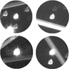 |
Fig. 1 Satellite trail examples visible on CHEOPS images. The main instrument is purposely defocused to spread a star’s light over many detector pixels, which increases the precision of its brightness measurements by minimizing errors from pixel-to-pixel variations and slight pointing instabilities. |
2 Methods
2.1 Data
In this work, we utilized the Level 1 Corrected Subarray data cubes (SCI_COR_SubArray) produced by the CHEOPS Data Reduction Pipeline (DRP). These files are provided as 3D data cubes containing the full time-series of subarray images acquired during each time-series observation. Each slice of the cube represents a 200x200 pixel window centered on the target, which has been corrected for instrumental effects (bias, gain, dark current, flat-field) and environmental factors (hot pixels and cosmic rays). To reduce data volume, the onboard software applies a circular cropping mask with a diameter of 200 pixels to these windows prior to downlink. These image cubes serve as the direct input for the final photometry module, which extracts the Level 2 photometric light curves that are the main high-level scientific product delivered by CHEOPS.
The individual images within the datacubes (the images analyzed for this work) result from the onboard coaddition of shorter individual exposures. The individual exposure time was selected to avoid any saturation of the detector pixels. Consequently, the effective integration time of the analyzed frames was determined by the individual exposure time and the number of combined frames. All archival images feature effective exposure times of 60 seconds or less, with 60% of the images having a precise 60-second integration time and 95% of the total archive above 30 seconds.
The CHEOPS telescope is intentionally defocused to spread the stellar point spread function (PSF) over a radius of approximately 16.5 pixels2, which increases the photometric stability required for exoplanet transit detection minimizing pixel-to-pixel variations and mitigating pointing instabilities. A direct consequence of this optical configuration is that all sources, including artificial satellites, appear as broad features on the detector. This characteristic defocus affects the detectability of trails by imposing a unique morphological signature: satellite trails appear as wide streaks, often inheriting features from the PSF’s particular shape. This structural complexity serves as a distinct advantage for a neural network, allowing it to effectively differentiate satellite trails from sharp artifacts such as cosmic rays.
2.2 The neural network model
To identify images featuring satellite trails, we created a binary image classifier model, using the MobileNetV2 architecture (Sandler et al. 2018) as our backbone. This selection was primarily driven by the critical need for computational efficiency, making it well suited for real-time applications and deployment on resource-constrained platforms such as satellite or mission on-board processing. Its architecture employs inverted residual blocks and linear bottlenecks to significantly reduce the number of parameters and floating-point operations compared to larger, more complex networks. This design is key for facilitating rapid inference speeds without a prohibitive sacrifice in model performance.
To tailor the model for our specific task, the MobileNetV2 based architecture was augmented with a custom classification head. This expansion is necessary to translate the high-level feature maps extracted by the backbone into a specific binary decision boundary for trail detection, while preserving the model’s overall computational efficiency. The head is composed of the following sequential layers, built with standard deep learning components (Goodfellow et al. 2016):
Global Average 2D Pooling layer: this layer is utilized to drastically reduce the total number of trainable parameters, aiding computational speed. It also averages out spatial dimensions, making the network robust to the spatial translations of satellite trails across different regions of the image frame.
Dropout layer with a rate of 0.5 for regularization: this serves as a critical preventive measure against overfitting. By randomly deactivating half of the neurons during training, it forces the network to learn generalized features rather than memorizing the training set.
Dense layer with 1024 neurons, using ReLU as its activation function and a 12 kernel regularizer: this layer provides the necessary non-linear capacity to learn complex combinations of the extracted features. The 12 regularizer helps to further suppress overfitting.
Final single-neuron Dense prediction layer employing a Sigmoid activation function to output the classification probability: this is the standard requirement for binary classification, mapping the final representations into a continuous classification probability between 0 and 1 to indicate the presence of a satellite trail.
2.3 Training the model
To train our model, we needed a dataset containing positive and negative examples: images containing satellite trails and images not featuring any. For the positive identifications, we used the images identified as presenting satellites from Gonçalves et al. (2026), for a total of 4747 images. Regarding the negative set, during our first training iteration, we randomly selected 4730 images from the full CHEOPS archive (not including the positive identifications set). This first model was used for a first test run classifying the whole public CHEOPS archive (April 2025, 1 680 467 images). A total of 14 964 images were identified as containing a satellite by the model. We defined a positive detection as an image with a probability of containing a satellite higher than 0.8 (this choice is further developed in Section 3.1).
A visual inspection of the results revealed a very high occurrence rate of false positives. Specifically, the model erroneously flagged approximately 2200 anomalous images as containing satellites. The reason for this high false-positive rate is statistical: instrumental and observational artifacts represent a very small fraction of the total public archive (1 680 467 images). Consequently, a purely random sample of 4730 negative images is highly unlikely to contain a representative set of these “hard negatives”. Because the algorithm rarely encountered these specific artifacts during its initial training, it failed to recognize and reject them during archive-wide inference.
A detailed manual inspection of these false positives showed that the algorithm primarily struggled with features resembling straight lines. These challenging cases included observations close to the Earth’s limb, images containing significant amounts of stray light, crowded fields with background sources coincidentally forming lines, and exceptionally bright sources3. The model also flagged trails caused by saturated sources both inside and outside the cropped images (CHEOPS SCI images are automatically cropped from a larger CCD, as explained in Benz et al. (2021) and its observer manual4), as well as internal reflections from nearby bright stars, atmospheric refraction (i.e., when the line of sight gets too close to the Earth’s limb) and cosmic rays. We show some examples of these special cases in Figure 2
To mitigate these false positives, we employed an approach combining systematic filtering and model retraining. A first subset of these artifacts could be systematically filtered out from the results using simple methods: images heavily affected by the Earth’s limb or stray light were removed using a background value threshold, while readout effects were identified by filtering for vertical trails strictly aligned with the pixel columns. Furthermore, artifacts caused by saturated sources (both inside and outside the cropped image) could be identified by exploiting the spacecraft’s specific viewing geometry. Because CHEOPS is nadir-locked, the spacecraft continuously rotates around the telescope’s line of sight during an observation. Consequently, these artifacts rotate systematically with the field of view. We successfully filtered these cases by selecting image sequences where the variation in the detected trail angle matched the CHEOPS roll angle.
The remaining false positives, predominantly corresponding to crowded fields, complex refractions, and internal reflections, could not be easily isolated using systematic filters. Instead, we gathered this specific subset of images and injected them back into our negative training set. By using these isolated cases to train a new algorithm, we drastically improved the model’s robustness and precision against these highly challenging observational scenarios.
Nevertheless, using all the manually selected false positives to train a new model would have been no different than manually cleansing our results, given that all the potential false positives that the model will encounter when classifying the archive are shown to it beforehand. To avoid this, we selected approximately half of them, which we then used to improve our model and test its ability to generalize and correctly filter false positives it had never seen before.
The final training set version includes the original 4747 images from the original positive set and a boosted 5748 negative set, containing the original 4730 random no-satellite images and an additional set of 1018 images featuring false positive cases.
We selected a 70-15-15 split for the training, validation and test sets. To improve model generalization and prevent overfitting, we employed on-the-fly data augmentation during training. The augmentation pipeline included a series of random geometric and photometric transformations: rotations (up to 20°), width and height shifts (up to 20%), shearing (up to 0.2 intensity), zooming (up to 20%), horizontal flips, and brightness adjustments (within a 80 and 120% range).
Regarding the training process itself, as illustrated in Figure 3, the model’s metrics for accuracy and loss converged steadily. The y-axes quantify two dimensionless metrics. For the top chart, it represents binary cross-entropy loss, measuring prediction error based on the difference between the model’s probability scores and the actual outcomes (Shannon & Weaver 1949; Goodfellow et al. 2016). For the bottom chart, it represents accuracy, the proportion of samples correctly identified by the model. An early stopping method was used to prevent overfitting, stopping the process after four consecutive epochs showed no reduction in validation loss, with the final model being selected from epoch 18 based on optimal validation performance.
The model’s classification performance on the test set (images never seen by the model before) is summarized in the confusion matrix shown in Figure 4. From a total of 1574 test samples, the model correctly classified 1562 instances, achieving an overall accuracy of 99.2%.
Satellite class (positive class): The model correctly identified 710 out of 712 satellite images, resulting in a recall (sensitivity) of 99.7%.
No satellite class (negative class): The model correctly identified 852 out of 862 images without satellites, achieving a specificity of 98.8%.
The precision for the satellite class was 98.6%, meaning that when the model predicted an image contained a satellite, it was correct 98.6% of the time. The values for both precision and recall resulted in a balanced F1-score of 99.2%.
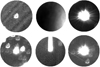 |
Fig. 2 Examples of false positives identified by the first version of our algorithm. Clockwise from top-left: stray light pattern, pointing errors too close to the Earth’s limb, very bright sources, cosmic rays, atmospheric refraction, and crowded fields. |
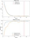 |
Fig. 3 Model training and validation history. The plots show the loss (top) and the accuracy (bottom) over the training epochs. The vertical dashed line indicates the point at which early stopping was triggered, epoch 18. Both loss and accuracy are dimensionless quantities. |
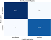 |
Fig. 4 Confusion matrix of the model’s classification performance on the test set. |
3 Results
3.1 Classifying the CHEOPS archive
Using the improved machine learning model, we classified the whole public CHEOPS Archive (1 801 211 images, up to June 2025) and obtained 12 268 positive satellite identifications, defined as images with a satellite probability score above 0.8.
This conservative threshold was chosen deliberately given the fact that within a massive and highly imbalanced dataset such as the CHEOPS archive, lower probability thresholds inherently increase the risk of capturing ambiguous artifacts. A quantitative assessment on our test set revealed that lowering the threshold to a more permissive 0.5 yields an almost identical overall accuracy, with a negligible difference of less than 0.06%. However, because the archive is overwhelmingly dominated by images without satellites, this small statistical difference translates to roughly a thousand doubtful, low-confidence detections when scaled across 1.8 million frames. Enforcing the stricter 0.8 threshold ensures the highly reliable identification of satellite trails while successfully avoiding the extensive inproduction manual vetting that would otherwise be required to filter out these borderline predictions. Furthermore, prioritizing high-confidence autonomous detections makes the algorithm highly suitable for future on-board processing applications, where human intervention to filter low-probability positives is impossible.
We visually inspected all these positively flagged images to verify the reliability of our method, which allowed us to manually identify and remove 45 false positives, representing 0.3% of the total detections, a figure that is consistent with the previously presented test set results. This new iteration of the model demonstrates a significant improvement in terms of generalization, using just half of the original false positives for training. This means that we are now able to correctly reject most of the special cases of different phenomena similar to satellite trails.
The total number of images featuring artificial satellite trails is 12 223, representing 0.68% of the CHEOPS archive. This figure is higher than the results from the study presented by Billot et al. (2024), probably due to the higher sensitivity of the machine learning algorithm (see Section 3.3) and the increase in the number of satellites in orbit.
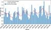 |
Fig. 5 Percentage of images per month featuring artificial satellites between Feb. 2020 and Jun. 2025. The red curve shows the six-month rolling average and the gray dotted line the linear trend for this average. |
3.2 Detection statistics
We show the monthly percentage of images with satellite detections over the total number of images in Figure 5. The red curve shows the 6-month rolling average value. We observe a stable increasing trend during recent years, bringing the peak average close to 1% of the monthly images for the worst period. This histogram displays seasonal variations, particularly a severe detection deficit during the winter season in the northern hemisphere. This occurs as the spacecraft’s orbit (inclination ≈ 98 degrees) enters an eclipse season, frequently placing both CHEOPS and other artificial satellites in its field of view within Earth’s shadow.
Each detection was analyzed using the trail analysis pipeline from Gonçalves et al. (2026) to extract parameters such as trail geometric parameters and brightness. For object identification, we cross-matched our detections with the Space-Track artificial satellites database5. For each detection, we first computed CHEOPS position using its two-line element (TLE) set closest in time. We then selected the TLE closest to the observation time from all available orbits within a 96 h window around the observation time and predicted the positions of all candidate objects within a 250 arcsec radius of the CHEOPS pointing coordinates. This search radius was conservatively chosen to account for the inherent inaccuracies of TLE propagation. Because CHEOPS and the target satellites could be in close orbital proximity, a TLE spatial error of ≈1 km could translate to angular uncertainties of several hundred arcseconds. We also implemented a directional constraint by calculating the position angle difference between the detected trail and the projected TLE. We also took into account CHEOPS’ roll angle and the candidate satellite’s specific orbital trajectory. A positive correlation was assumed only if the predicted angle of the candidate’s movement varied by no more than 6 degrees from the observed trail angle.
If the algorithm could not reliably identify the trail parameters (e.g., in the case of dim or wide, irregularly structured trails), we used a relaxed criterion, keeping the best match within a 350 arcsec radius. To complement the analysis for fainter sources, which are more prone to error, we applied a goodness-of-fit threshold to our detections. We determined the fit quality through the chi-squared residual (CSR) between the observed trail profile and the candidate’s theoretical trajectory.
Post-processing of our 12 223 images yielded 22 830 candidate trail identifications. To eliminate potential spurious or ambiguous cases, we assessed identification validity using the calculated CSR values. We employed an interquartile range (IQR) outlier detection method (Tukey 1977) to filter these spurious associations6, which retained 19875 detections. From this filtered set, 9176 detections matched valid and unique NORAD IDs in the Space-Track database. To determine object characteristics, such as type or size, we utilized the IAU-CPS SatChecker tool7 to retrieve metadata associated with these NORAD IDs; successful retrieval was achieved for 7319 objects. Figure 6 illustrates the distribution of this dataset by object type and radar cross-section (RCS).
Overall, our 9176 matched detections correspond to 5565 distinct objects. Given the number of unmatched trails, the subset of objects lacking available metadata (including uncatalogued space debris or undeclared satellites), we cannot reliably determine the exact orbital classification of the observed population. As an order-of-magnitude reference, our matched sample size is roughly equivalent to 21% of the 26 671 estimated objects currently intersecting LEO orbits8. However, CHEOPS’s viewing geometry is not restricted to LEO. While the spacecraft orbits at an altitude of ~700 km, its pointing constraints allow a limiting downward line of sight with a projected tangent altitude of 100 km above the Earth’s surface. Furthermore, the telescope’s pointing is restricted to within 60 degrees of the anti-Sun direction. Consequently, the telescope’s field of view intersects higher orbital regimes, such as geostationary (GEO) and medium Earth orbit (MEO), along with all LEO shells down to 100 km. This geometry, combined with the complex illumination phenomena inherent to observing over the Earth’s night side, enables the detection of objects across a wide range of altitudes, both above and below the spacecraft.
The subset of objects with available metadata is composed primarily of payloads, followed by rocket bodies and debris. Across all three types, objects with a large size are the most numerous. While medium and small objects are present in all categories, they represent a proportionally much larger fraction of the debris population compared to payloads and rocket bodies. RCS is defined as small for RCS < 0.1 m2, medium for 0.1 < RCS < 1.0 m2 and large for RCS > 1.0 m2.
Finally, our phase angle statistics align excellently with the statistics from Billot et al. (2024) (Figure 7). The CHEOPS’ observable phase angle range is 0°–60°, corresponding to observations within 60° of the anti-Sun direction. As anticipated, most of our detected objects fall within an interval of low phase angles. The scarcity of objects observed near 0° phase angle is consistent with the lack of available images at that specific angle, a limitation also noted in the Billot et al. (2024) study. Section 3.4 gives more details about the magnitude of the objects.
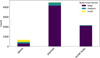 |
Fig. 6 Population breakdown (7319 objects). The stacked bar chart shows the total counts for each object type, subdivided by their RCS size. |
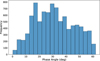 |
Fig. 7 Phase angle of our NORAD identifications set (9176 objects). |
3.3 Method comparison
It is of great importance to examine the two existing methods for identifying space debris in CHEOPS images (linear features detection algorithms or AI) to pinpoint their limitations and understand how these affect the choice of the most appropriate solution for a particular situation. We characterized each method in terms of the number of detections (Ndetections); the brightness limit (Blim), which corresponds to the peak on the detection brightness histogram before the detections start to fade (see Figure 8); the time required to process a single image (timage); and the false positive rate (FP) and if it can directly obtain trail geometric characteristics, also known as line information. The brightness is determined through line fitting, given CHEOPS’ PSF and the line information, as described in Gonçalves et al. (2026). Line information is the (ρ, θ), which give us the position and orientation of the line according to
![Mathematical equation: $\[\rho=x ~\cos~ \theta+y ~\sin~ \theta .\]$](/articles/aa/full_html/2026/04/aa58532-25/aa58532-25-eq1.png) (1)
(1)
The comparative classification of both techniques is illustrated in Table 1. It is important to note that the absolute total number of detections (NDetections) reflects the different archival periods analyzed by each respective study; the ML method encompasses the archive up to June 2025, whereas the classic method figures reflect the earlier baseline established by Gonçalves et al. (2026) up to October 2022. However, a direct and fair comparison of the algorithms’ performance is achieved by examining the detection rates during their overlapping time-frames. As illustrated previously in Figure 5, our ML approach consistently achieves a higher monthly detection percentage (≈0.68%) compared to the overall rates reported by Gonçalves et al. (2026) (≈0.33%) for the exact same historical periods. This higher overall detection yield is a direct consequence of the ML method’s superior sensitivity, which is also depicted in Table 1 by its significantly lower brightness limit.
The ML method achieves a higher number of detections than the classic model, as it can detect fainter sources. Its main disadvantage is the longest processing time required to analyse each image, which necessitates the use of hardware acceleration to maintain a manageable processing time; and not directly obtaining the trail’s line characteristics (ρ, θ).
This time factor has no impact if the acquisition rate remains below the analysis rate. This applies to the CHEOPS case, where observations are typically long (30–60 s). However, for dedicated space missions aiming to maximize acquisition rates, this latency could prove to be a limiting factor. Currently, ESA’s VISDOM mission (Kraft et al. 2024), designed to demonstrate in-orbit optical technology for space debris monitoring, targets a 0.67 Hz frame rate; consequently, it would not be impacted by the presented processing time. Nevertheless, as frame rates increase for future missions, this overhead may become a bottleneck.
The hardware factor limits applicability for smaller systems, as it requires an onboard graphics processing unit (GPU), which may exceed typical power constraints. However, this is a mission-specific condition and future technological developments may mitigate this disadvantage. In contrast, ground facilities do not face any problems in implementing this acceleration. Finally, the development of lightweight ML detection algorithms specifically tailored for onboard processing remains a promising direction. Optimization strategies such as quantization, which reduces the numerical precision of model weights and activations from 32-bit floating-point to 8-bit integers (Jacob et al. 2017), significantly reduce memory footprint and inference latency. This combination enables high-accuracy detection on low-power hardware accelerators, such as vision processing units (VPUs) as demonstrated in the Φ-Sat-1 mission (Giuffrida et al. 2022), rather than relying on power-intensive GPUs.
The direct line characterization factor presents no disadvantage if the objective is limited to pure object detection. However, advanced studies requiring detailed line analysis (such as brightness determination) would necessitate applying the classic method within a two-step pipeline
The ML outperforms the classic model by a significant margin in terms of detection limit, which is key for catalogue completion, without sacrificing accuracy with the added training subset. It is the method of choice if hardware requirements and frame rate are not an issue. However, the computational expense associated with the classic method is minimal compared to that of the ML approach. Consequently, synergies can be obtained by applying the classic method to separate frames, while using the ML method for ≥1 second stacks. This strategy has the potential to combine the enhanced frame rate of the classic method with the greater depth offered by the ML approach.
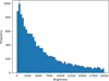 |
Fig. 8 Histogram showing the brightness of all trails detected by the ML method, with the peak highlighted with a green vertical line. The X axis unit is counts. |
Characteristic comparison between classic and ML models.
3.4 Brightness analysis
Artificial satellite brightness has raised concerns regarding dark-sky preservation, both for the general population and scientific missions, which might face significant limitations or even total disruption in the future. This has prompted communication between satellite operators and manufacturers and the Dark Sky community to reduce the apparent magnitude of artificial satellites. Leveraging our dataset spanning several years (2020-2025), we analyzed the variation in brightness of the detected objects over time. We used the standard magnitude (mstandard) as opposed to the apparent magnitude (mapparent) because it is independent of the distance at which the object is observed, which can change significantly from observation to observation. This is determined by
![Mathematical equation: $\[m_{standard}=m_{apparent}-5 ~\log \left(\frac{d}{1000}\right) \text {, }\]$](/articles/aa/full_html/2026/04/aa58532-25/aa58532-25-eq2.png) (2)
(2)
where d is the distance from CHEOPS to the object in km and mapparent is determined through the trail analysis pipeline from Gonçalves et al. (2026). This pipeline extracts the trail’s brightness via a point spread function line fit to the satellite streak. This measurement is then calibrated against the central target star using standard CHEOPS PSF calibration files, the exposure time, and the satellite’s velocity.
In Figure 9, we illustrate the histograms representing the standard magnitude of the objects across the different observation years. We obtained a global mean value of 13.4 with a standard deviation of σ = 1.7. Additionally, in Figure 10, we depict the standard magnitude over time.
There are no visible differences in the magnitude values for the different years. However, this could be due to the fact that detections are dominated by older satellites that have not yet decayed. To study this hypothesis, we plot the standard magnitude versus the object launch date as shown in Figure 11.
This figure shows that objects’ brightness slightly increases over the years if we take into account their launch date, accompanied by a great increase in launch density. While this could be correlated with the deployment of new satellite types presenting more reflectance from space, another significant factor contributing to this trend could be the material degradation of older objects due to prolonged exposure to the space environment. Research indicates that the harsh in orbit conditions alter the properties of spacecraft surfaces over time, resulting in the erosion of surface coatings and the darkening of insulation layers and solar cell cover glasses, thereby reducing their diffuse reflectance and overall albedo (Miller & Banks 2011; Messenger & Kruer 2018). A special note needs to be added that space and ground-based observations might create slightly different results, as satellite geometry might be constructed to minimize reflections to ground observers, which might then increase for space observers. However, we argue that specular reflections would account for outliers on the brighter side of the graph, whereas the median value is more representative of purely diffuse reflection.
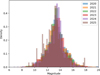 |
Fig. 9 Standard magnitude distribution of detected objects for each year of the CHEOPS database. |
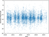 |
Fig. 10 Standard magnitude of detected objects over the years in the CHEOPS database. |
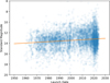 |
Fig. 11 Standard magnitude of detected object versus launch date of object with trend line showing an increasing brightness trend over time. |
4 Conclusions
Ensuring the scientific integrity of high-precision photometric data requires the effective identification and exclusion of transient contaminants. In this work, we demonstrate that AI-driven approaches are highly effective for flagging satellite trails to preserve the value of astronomical images. We have developed, trained, and validated a computationally efficient artificial intelligence algorithm based on the MobileNetV2 architecture to detect artificial satellite trails in images from the CHEOPS space telescope. Our primary objective was to create a robust classifier for this specific task and benchmark its performance against traditional, non-AI-based linear feature detection methods.
A critical finding of this study was the necessity of an iterative training process. An initial model trained on randomly selected negative (no-satellite) images suffered from a high false-positive rate when applied to the full archive, incorrectly identifying features such as stray light, cosmic rays, and crowded stellar fields. By creating an enhanced training set, which incorporated a curated sample of these hard-negative cases, our final model achieved an overall accuracy of 99.2% on the test set. This robustness was confirmed by classifying the entire 1.8 million CHEOPS image archive (up to June 2025), where the final false-positive rate was only 0.3%.
This sensitive AI-driven survey identified 12 223 images containing satellite trails, corresponding to 0.68% of the entire public CHEOPS archive. This detection rate confirms a stable, slightly increasing trend in satellite interferences, peaking near 1% of monthly images during the worst periods, and it corroborates seasonal variation patterns noted in prior work. Furthermore, through cross-matching with the Space-Track database, we successfully associated our detections with 5565 unique objects, demonstrating the potential of CHEOPS as a serendipitous space surveillance sensor.
A direct comparison with legacy, classic non-AI linear feature identification methods highlights a clear trade-off. Our AI algorithm is demonstrably more sensitive, more than doubling the number of detections compared to previous studies on the same archive. However, classic methods remain significantly faster and do not require GPU acceleration, making them advantageous for on-board, resource-constrained, or real-time applications where extreme sensitivity is secondary to processing speed.
Our photometric analysis provides key insights into the evolving optical characteristics of the satellite population. While the average standard magnitude of detections across the 2020–2025 period has remained relatively constant (13.4 ± 1.7), a correlation with launch dates reveals that recently launched objects tend to be brighter than older ones. This suggests that older objects may undergo “darkening” due to material degradation and space weathering, while new launches maintain higher reflectivity.
Finally, it is important to assess the practical impact of these detection rates on CHEOPS’s primary scientific objectives. Currently, a contamination peak of ~1% remains manageable. CHEOPS’s final data products are calibrated time-series measurements extracted from sequences of short exposures (≤60 seconds). Consequently, satellite trails typically manifest as isolated outliers. Because the exoplanet transits occur on much longer timescales, these sporadic outliers are generally filtered out during standard light-curve analysis. Nevertheless, the rapid expansion of the satellite population means this interference will increase. Implementing efficient automated flagging tools, such as the AI algorithm presented here, will become increasingly necessary to maintain data quality in the near future.
Acknowledgements
Computational aspects of this work were supported by a grant from the Google Cloud Research Credits Program. This research made use of the ESA Datalabs environment for accessing and processing data from the CHEOPS scientific archive. This publication makes use of The Data & Analysis Center for Exoplanets (DACE), which is a facility based at the University of Geneva (CH) dedicated to extrasolar planets data visualisation, exchange and analysis. DACE is a platform of the Swiss National Centre of Competence in Research (NCCR) PlanetS, federating the Swiss expertise in Exoplanet research. The DACE platform is available at https://dace.unige.ch. The authors acknowledge the use of Google Gemini for language editing and styling of the text. The authors reviewed and edited the output as needed and take full responsibility for the content of the publication.
References
- Benz, W., Broeg, C., Fortier, A., et al. 2021, Exp. Astron., 51, 109 [Google Scholar]
- Billot, N., Hellmich, S., Benz, W., et al. 2024, J. Space Saf. Eng., 11, 498 [Google Scholar]
- Boley, A. C., Green, R., Rawls, M. L., & Eggl, S. 2025, RNAAS, 9, 60 [Google Scholar]
- Dhinakaran, A., Nadaraja Pillai, S., Shahul Hameed, V., & Priya, S. B. M. 2025, Acta Astronaut., 236, 281 [Google Scholar]
- Dillmann, S., Martínez-Galarza, J. R., Soria, R., Di Stefano, R., & Kashyap, V. L. 2025, MNRAS, 537, 931 [Google Scholar]
- García-Martín, P., Kruk, S., Popescu, M., et al. 2024, A&A, 683, A122 [NASA ADS] [CrossRef] [EDP Sciences] [Google Scholar]
- George, D., & Huerta, E. A. 2018, Phys. Lett. B, 778, 64 [NASA ADS] [CrossRef] [Google Scholar]
- Giuffrida, G., Fanucci, L., Meoni, G., et al. 2022, IEEE Trans. Geosci. Remote Sens., 60, TGRS.2021 [Google Scholar]
- Gonçalves, L. F. P., Billot, N., Hellmich, S., et al. 2026, Acta Astronaut., 239, 61 [Google Scholar]
- Goodfellow, I., Bengio, Y., & Courville, A. 2016, Deep Learning (Cambridge, MA: MIT Press) [Google Scholar]
- Hainaut, O. R., & Moehler, S. 2024, A&A, 683, A147 [NASA ADS] [CrossRef] [EDP Sciences] [Google Scholar]
- Hasan, I., Tyson, J. A., Saunders, C., & Xin, B. 2022, Astron. Comput., 39, 100584 [Google Scholar]
- Hu, J. A., Rawls, M. L., Yoachim, P., & Ivezić, Ž. 2022, ApJ, 941, L15 [NASA ADS] [CrossRef] [Google Scholar]
- Irureta-Goyena, B. Y., Helou, G., Kneib, J.-P., et al. 2025, PASP, 137, 054503 [Google Scholar]
- Jacob, B., Kligys, S., Chen, B., et al. 2017, arXiv e-prints [arXiv:1712.05877] [Google Scholar]
- Jenkins, M. 2024, Space Educ. Strateg. Appl., 4, 4 [Google Scholar]
- Kraft, S., Scoubeau, M., Biswas, I., et al. 2024, in 22nd IAA Symposium on Space Debris (Paris: International Astronautical Federation (IAF)), 71 [Google Scholar]
- Kruk, S., García-Martín, P., Popescu, M., et al. 2023, Nat. Astron., 7, 262 [CrossRef] [Google Scholar]
- Liou, J. C., Johnson, N. L., & Hill, N. M. 2010, Acta Astronaut., 66, 648 [Google Scholar]
- Messenger, S. R., & Kruer, M. A. 2018, IEEE Trans. Nucl. Sci., 65, 149 [Google Scholar]
- Miller, S. K. R., & Banks, B. 2011, MRS Bull., 35, 20 [Google Scholar]
- Sandler, M., Howard, A., Zhu, M., Zhmoginov, A., & Chen, L.-C. 2018, arXiv e-prints [arXiv:1801.04381] [Google Scholar]
- Shallue, C. J., & Vanderburg, A. 2018, AJ, 155, 94 [NASA ADS] [CrossRef] [Google Scholar]
- Shannon, C. E., & Weaver, W. 1949, The Mathematical Theory of Communication (Urbana: University of Illinois Press) [Google Scholar]
- Stark, D. V., Grogin, N., Ryon, J., & Lucas, R. 2022, Improved Identification of Satellite Trails in ACS/WFC Imaging Using a Modified Radon Transform, Instrument Science Report ACS 2022-8, 25 [Google Scholar]
- Tukey, J. W. 1977, Exploratory Data Analysis (Boston, MA: Addison-Wesley Publishing Company) [Google Scholar]
- Tyson, J. A., Ivezić, Ž., Bradshaw, A., et al. 2020, AJ, 160, 226 [Google Scholar]
The radius of the PSF is calculated as the radius of a circle that contains 90% of the flux.
CHEOPS camera is shutterless and very bright targets show vertical blurring due to the readout process.
Defining the rejection threshold as Q3 + 1.5 · IQR.
All Tables
All Figures
|
Fig. 1 Satellite trail examples visible on CHEOPS images. The main instrument is purposely defocused to spread a star’s light over many detector pixels, which increases the precision of its brightness measurements by minimizing errors from pixel-to-pixel variations and slight pointing instabilities. |
| In the text | |
|
Fig. 2 Examples of false positives identified by the first version of our algorithm. Clockwise from top-left: stray light pattern, pointing errors too close to the Earth’s limb, very bright sources, cosmic rays, atmospheric refraction, and crowded fields. |
| In the text | |
|
Fig. 3 Model training and validation history. The plots show the loss (top) and the accuracy (bottom) over the training epochs. The vertical dashed line indicates the point at which early stopping was triggered, epoch 18. Both loss and accuracy are dimensionless quantities. |
| In the text | |
|
Fig. 4 Confusion matrix of the model’s classification performance on the test set. |
| In the text | |
|
Fig. 5 Percentage of images per month featuring artificial satellites between Feb. 2020 and Jun. 2025. The red curve shows the six-month rolling average and the gray dotted line the linear trend for this average. |
| In the text | |
|
Fig. 6 Population breakdown (7319 objects). The stacked bar chart shows the total counts for each object type, subdivided by their RCS size. |
| In the text | |
|
Fig. 7 Phase angle of our NORAD identifications set (9176 objects). |
| In the text | |
|
Fig. 8 Histogram showing the brightness of all trails detected by the ML method, with the peak highlighted with a green vertical line. The X axis unit is counts. |
| In the text | |
|
Fig. 9 Standard magnitude distribution of detected objects for each year of the CHEOPS database. |
| In the text | |
|
Fig. 10 Standard magnitude of detected objects over the years in the CHEOPS database. |
| In the text | |
|
Fig. 11 Standard magnitude of detected object versus launch date of object with trend line showing an increasing brightness trend over time. |
| In the text | |
Current usage metrics show cumulative count of Article Views (full-text article views including HTML views, PDF and ePub downloads, according to the available data) and Abstracts Views on Vision4Press platform.
Data correspond to usage on the plateform after 2015. The current usage metrics is available 48-96 hours after online publication and is updated daily on week days.
Initial download of the metrics may take a while.