© The Authors 2026

1. Introduction

Solids in protoplanetary discs drift towards regions of higher pressure (Safronov 1972). As such, pressure maxima (often called pressure bumps) are primary locations for collecting solids and fostering planet formation (e.g. Bae et al. 2023; Lesur et al. 2023; Drażkowska et al. 2023). Locating and characterising such features of great interest to the planet formation community. While dust can be directly imaged, the gas made of H₂ is mostly invisible and requires tracers. The gas pressure profile has recently been quantitatively constrained from inverting the mean rotational profile, using high-precision kinematic data of CO emission lines obtained with the Atacama Large Millimeter/submillimeter Array (ALMA) (e.g. Pinte et al. 2023). Departures from circular Keplerian motion can arise from pressure gradients, disc eccentricity or inclination, secondary flows, or additional physical processes such as self-gravity, dust dynamics, or magnetic fields (e.g. Teague et al. 2025). These processes, together with the presence of protoplanets, shape the pressure profile of the gas into a structured disc, with pressure bumps and dips (e.g. as observed by van Capelleveen et al. 2025). Probing this flow and these processes by a seismic analysis could be achieved with spatially or time-resolved kinematic data: this is the very goal of discoseismology, essentially introduced so far to study accretion discs around black holes (Solheim et al. 1998; Tsang & Lai 2009; Tsang & Butsky 2013; Ortega-Rodríguez et al. 2020; Dewberry et al. 2020a,b; Kato 2024). This approach is aimed at constraining the structure of the disc not via the mean flow, but through the study of linear perturbations about its equilibrium.

Linear waves and instabilities have a well-established history as mechanisms for forming structures in discs (Toomre 1964; Goldreich & Lynden-Bell 1965a; Lynden-Bell & Ostriker 1967; Papaloizou & Pringle 1985); for instance, the spiral arms of galaxies are understood to be density waves (Lin & Shu 1966; Lynden-Bell & Kalnajs 1972). External perturbers can excite both inertial and acoustic waves at Lindblad resonances, where the orbital period of the mean flow is commensurable with the perturbation’s period, which launches waves in the disc (Lindblad 1948; Goldreich & Tremaine 1978, 1979; Lubow & Ogilvie 1998). This occurs in Saturn’s rings, where ring waves in resonance with oscillations of the planet have been observed by Cassini, which provided the first and only seismic data on Saturn (Marley 1991; Hedman & Nicholson 2013; Fuller 2014).

While global modes of isothermal and polytropic discs have been widely investigated (Kato & Fukue 1980; Kato 1983; Papaloizou & Pringle 1985; Blaes 1985; Blaes et al. 2006, 2007), the analysis becomes simpler when focusing solely on small-scale perturbations within the shearing-box framework, where the fluid evolution is described in a small cartesian box rotating with the flow (Hill 1878; Goldreich & Lynden-Bell 1965b). This has led to important advances in our understanding of wave propagation, instabilities, turbulence, angular-momentum transport, and planetesimal formation in accretion and protoplanetary discs (e.g. Kato 1978; Goldreich & Tremaine 1980; Balbus & Hawley 1991; Lubow & Pringle 1993; Goodman 1993; Korycansky & Pringle 1995; Ogilvie 1998; Balbus & Hawley 1998; Ogilvie & Lubow 1999; Youdin & Goodman 2005; Johansen et al. 2007; Nelson et al. 2013).

On the other hand, as is the case for stellar seismology (e.g. Aerts et al. 2010), the key targets for discoseismology are large-scale global modes, since they probe the overall structure of the disc and are the easiest to detect. Among these, topological modes are especially attractive, since they can be studied and constrained without the need for short-wavelength or local techniques. These modes stem from a topological property of the differential operator that governs their evolution. While such modes have been investigated for decades in condensed-matter physics, their study in hydrodynamics has emerged only recently (Delplace et al. 2017; Perrot et al. 2019; Perez et al. 2022, 2025; Parker et al. 2020; Qin & Fu 2023). Since topological analysis has not received much attention in astrophysical fluids to date, characterisations of topological modes may enable new methods of probing the structure of interesting objects. The example of topological waves in stars is to this respect particularly instructive. Leclerc et al. (2022) demonstrated that the cancellation of a particular characteristic frequency in stars necessarily gives rise to a topological mode, explaining why f-branch modes with small harmonic degrees are not confined to the stellar surface. These modes were subsequently shown to remain robust in the presence of convective regions and radiative dissipation, and they are excited by convective motions (Leclerc et al. 2024a; Le Saux et al. 2025). They have also been observed to hybridise with g-modes, providing the most reliable method to date for inferring the rotation rate of the solar core (Le Saux et al. 2025). Stellar rotation was also found to induce topological modes in seismic spectra (Leclerc et al. 2024b). For details on the theory of wave topology for astrophysical and geophysical wave, we refer to Perez (2022) and Leclerc (2025). Building on these developments performed in the stellar context, we aim to address the following issues, namely: whether topological modes exist in discs and, if so, how they are related to the pressure profile. We address these questions here and highlight the special properties these modes have, suggesting how they might serve the interest for of protoplanetary disc seismology and dynamics. In Sect. 2 we begin by examining the local propagation of waves by performing a so-called micro-local analysis of the linear wave operator of a simple model of a disc to obtain the local dispersion relation as well as the local polarisation relations between the wave fields (Keppeler 2004; Hall 2013; Onuki 2020; Vidal & de Verdiére 2024). This marks the first time this method has been applied in the context of astrophysical discs. In Sect. 3 we exhibit the topological properties of the problem and predict the existence of topological modes. We then focus on the role of the presence of extrema in the pressure profile in Sect. 4, analysing how they are reflected in the spectrum of large-scale modes. Further extensions of this study are discussed in Sect. 5.

2. Local waves without a shearing box

2.1. Epicyclic-acoustic frequency

We considered an unstratified disc made of a non-self gravitating ideal gas around a star of mass M. The equations of motion for the velocity, v, pressure, p, and density, ρ, are

$$\begin{array}{cc}\hfill {\partial }_t\mathit{v}+(\mathit{v}·\mathrm{\nabla })\mathit{v}& =-\frac{1}{\rho }\mathrm{\nabla }p-\frac{\mathcal{G}M}{r^2}{\mathit{e}}_{\mathrm{r}},\hfill \end{array}$$(1)

$$\begin{array}{cc}\hfill {\partial }_t\rho +\mathrm{\nabla }·\left(\rho \mathbf{v}\right)& =0,\hfill \end{array}$$(2)

along with an appropriate energy equation. We restricted our analysis to the case of a circular disc. In cylindrical coordinates (r, θ, z), the equilibrium profile is parametrised by ρ = ρ₀(r), p = p₀(r), v = (0, rΩ(r),0), and does not depend on z as it is unstratified. Along the radial direction, we have

$$\begin{array}{c}\hfill r{\mathrm{\Omega }}^2=\frac{1}{{\rho }_0}\frac{\mathrm{d}{p}_0}{\mathrm{d}r}+\frac{\mathcal{G}M}{r^2}.\end{array}$$(3)

We linearly expanded the quantities as X = X₀ + X′ in Eqs. (1) and (2), assuming adiabatic axisymmetric perturbations of the gas (∂_tp′+∂_rP₀ v_r′=c_s²(∂_tρ′+∂_rρ₀ v_r′)). This is expressed as (Latter & Papaloizou 2017)

$$\begin{array}{cc}\hfill {\partial }_t{v}_{\mathrm{r}}^{\prime }& =2\mathrm{\Omega }{v}_{\theta }^{\prime }-\frac{1}{{\rho }_0}{\partial }_r{p}^{\prime }+\frac{p^{\prime }}{c_{\mathrm{s}}^2{\rho }_0^2}\frac{\mathrm{d}{p}_0}{\mathrm{d}r},\hfill \end{array}$$(4)

$$\begin{array}{cc}\hfill {\partial }_t{v}_{\theta }^{\prime }& =-(2\mathrm{\Omega }+r\frac{\mathrm{d}\mathrm{\Omega }}{\mathrm{d}r})v_{\mathrm{r}}^{\prime },\hfill \end{array}$$(5)

$$\begin{array}{cc}\hfill {\partial }_t{v}_z^{\prime }& =-\frac{1}{{\rho }_0}{\partial }_z{p}^{\prime },\hfill \end{array}$$(6)

$$\begin{array}{cc}\hfill {\partial }_t{p}^{\prime }& =-p_0(\frac{1}{r}{\partial }_{\mathrm{r}}(r{v}_{\mathrm{r}}^{\prime })+{\partial }_z{v}_z^{\prime })-\frac{\mathrm{d}{p}_0}{\mathrm{d}r}{v}_{\mathrm{r}}^{\prime }.\hfill \end{array}$$(7)

We applied the following change in variables,

$$\begin{array}{cc}\hfill (v_{\mathrm{r}}^{\prime },v_{\theta }^{\prime },v_z^{\prime })& \mapsto \mathit{u}\equiv \sqrt{r{\rho }_0}(v_{\mathrm{r}}^{\prime },\sqrt{\frac{2}{2-s}}{v}_{\theta }^{\prime },v_z^{\prime }),\hfill \end{array}$$(8)

$$\begin{array}{cc}\hfill p^{\prime }& \mapsto h\equiv \frac{\sqrt{r}}{\sqrt{{\rho }_0}{c}_{\mathrm{s}}}{p}^{\prime },\hfill \end{array}$$(9)

where $s\equiv \frac{\mathrm{d}ln\mathrm{\Omega }}{\mathrm{d}lnr}$. It reveals a symmetrised set of equations, which simplifies the subsequent choice of inner product introduced for the topological analysis (Leclerc et al. 2022; see our Sect. 2.2). Performing a Fourier transform e^{iωt − ik_zz} yields a wave equation for X^⊤ ≡ (u_z u_r u_θ h) of the form

$$\begin{array}{cc}& \mathcal{H}X=\omega X,\hfill \end{array}$$(10)

$$\begin{array}{cc}\hfill & \mathcal{H}=\hfill \\ \hfill & \left(\begin{array}{cccc}0& 0& 0& c_{\mathrm{s}}{k}_z\\ 0& 0& -i\kappa & i{c}_{\mathrm{s}}{\partial }_{\mathrm{r}}+\frac{i}{2}\frac{\mathrm{d}{c}_{\mathrm{s}}}{\mathrm{d}r}-iS\\ 0& i\kappa & 0& 0\\ c_{\mathrm{s}}{k}_z& i{c}_{\mathrm{s}}{\partial }_{\mathrm{r}}+\frac{i}{2}\frac{\mathrm{d}{c}_{\mathrm{s}}}{\mathrm{d}r}+iS& 0& 0\end{array}\right),\hfill \end{array}$$(11)

where $\kappa \equiv \sqrt{2(2-s)}\mathrm{\Omega }$ is the epicyclic frequency, while

$$\begin{array}{c}\hfill S\equiv \frac{c_{\mathrm{s}}}{2}(\frac{\mathrm{d}ln{p}_0}{\mathrm{d}r}+\frac{\mathrm{d}ln{c}_{\mathrm{s}}}{\mathrm{d}r}+\frac{1}{r})\end{array}$$(12)

denotes what we call the epicyclic-acoustic frequency of the disc, acting as a cutoff frequency (as we go on to show in the local dispersion relation). To the best of our knowledge, this is the first explicit identification of the frequency that governs momentum exchange between the inertial and acoustic bands in discs. Its expression follows directly from the rescaled symmetric Hermitian formulation of the wave equations. Here, S depends on the radial inhomogeneity and the curvature of the disc. Terms associated with Eq. (12) break the symmetry (r, u_r, u_θ)→ − (r, u_r, u_θ), which is only restored when S = 0. S plays the role, in discs, of the buoyant–acoustic frequency identified in stars by (Leclerc et al. 2022). For a stratified disc, this expression can be conveniently rewritten as

$$\begin{array}{c}\hfill S=\frac{1}{2}[\frac{\mathrm{d}ln{p}_0}{\mathrm{d}lnr}+\frac{\mathrm{d}ln{c}_{\mathrm{s}}}{\mathrm{d}lnr}+1]\frac{H_P}{r}\mathrm{\Omega },\end{array}$$(13)

where H_P ≡ c_sΩ⁻¹ is the pressure scale height of the disc.

We imposed impenetrable boundaries, such that u_r(r₀) = u_r(r₁) = 0. For a real κ (a Rayleigh stable disc), the operator ℋ is self-adjoint with respect to the canonical inner product ⟨X, Y⟩=∫dr X^†Y. The frequencies ω are then guaranteed to be real: the perturbations considered here are linearly stable. The self-adjointness of ℋ gives the following energetic constant of motion,

$$\begin{array}{cc}\hfill I& =\frac{1}{2}⟨X,X⟩,\hfill \end{array}$$(14)

$$\begin{array}{cc}& ={\displaystyle \int \mathrm{d}}r\frac{1}{2}({|\mathit{u}|}^2+{|h|}^2),\hfill \\ \hfill & ={\displaystyle \int \mathrm{d}}rr[\frac{1}{2}\rho (|v_{\mathrm{r}}^{\prime }{|}^2+\frac{2}{2-s}|v_{\theta }^{\prime }{|}^2+{|v_z^{\prime }|}^2)+\frac{1}{2\rho c_{\mathrm{s}}^2}{|p^{\prime }|}^2],\hfill \end{array}$$(15)

with proofs given in the appendices. The solutions to Eqs. (10) and (11), together with these boundary conditions, comprise the axisymmetric oscillation modes of the disc (i.e. the standing waves in the radial direction).

2.2. Local wave equation

A micro-local analysis is a representation of differential operators on a phase space using the Wigner transform (Keppeler 2004; Hall 2013). This transform maps (pseudo-)differential operators to ‘symbols’ (i.e functions of the phase space). Three useful symbols used here are

$$\begin{array}{cc}\hfill \mathrm{Symb}[c_{\mathrm{s}}(r)]& =c_{\mathrm{s}},\hfill \end{array}$$(16)

$$\begin{array}{cc}\hfill \mathrm{Symb}[i{\partial }_{\mathrm{r}}]& =k_{\mathrm{r}},\hfill \end{array}$$(17)

$$\begin{array}{cc}\hfill \mathrm{Symb}[i{c}_{\mathrm{s}}{\partial }_{\mathrm{r}}+\frac{i}{2}\frac{\mathrm{d}{c}_{\mathrm{s}}}{\mathrm{d}r}]& =c_{\mathrm{s}}{k}_{\mathrm{r}}.\hfill \end{array}$$(18)

This offers an appropriate way to define a local wavenumber, k_r, for a wave (Onuki 2020).

The operator, ℋ, is then mapped to its symbol, H,

$$\begin{array}{c}\hfill H=\left(\begin{array}{cccc}0& 0& 0& c_{\mathrm{s}}{k}_z\\ 0& 0& -i\kappa & c_{\mathrm{s}}{k}_{\mathrm{r}}-iS\\ 0& i\kappa & 0& 0\\ c_{\mathrm{s}}{k}_z& c_{\mathrm{s}}{k}_{\mathrm{r}}+iS& 0& 0\end{array}\right).\end{array}$$(19)

The Wigner transform has a number of useful properties, including the conservation of Hermiticity: ℋ is a self-adjoint differential operator if and only if H is a Hermitian matrix function (this property is detailed in Hall 2013, page 266). It can then guarantee that H gives the local dispersion relation of the waves without introducing spurious instabilities, as shown to happen when including pressure gradients in local studies (e.g. see the discussions in Lin & Youdin 2015 and Latter & Papaloizou 2017). Indeed, we have H^† = H. The local wave equation is

$$\begin{array}{c}\hfill HX=\omega X,\end{array}$$(20)

and the local dispersion relation can simply be obtained via det(H−ω𝟙) = 0, which yields

$$\begin{array}{c}\hfill c_{\mathrm{s}}^2{k}_{\mathrm{r}}^2=\frac{(c_{\mathrm{s}}^2{k}_z^2-{\omega }^2)({\kappa }^2-{\omega }^2)}{{\omega }^2}-S^2.\end{array}$$(21)

Equation (21) is a quadratic polynomial in ω², whose smaller root corresponds to the inertial band (or r-band) and the larger to the pressure band (or p-band). For the inertial waves, we have 0 ≤ ω² ≤ κ², while for the pressure waves, we have ω² ≥ κ² + S². Thus, a non-zero value of S opens a frequency gap between the bands and no wave with ω² ∈ (κ², κ² + S²) can propagate radially in the disc (see Fig. 1). The dispersion relation derived by other local expansions, which neglect both the curvature term and the pressure gradient, was recovered for S = 0. In that special case, there is a degeneracy between acoustic and inertial waves at ω = κ for (k_r, k_z) = (0, κ/c_s), but it is lifted by any non-zero value of S, that is, any non-zero pressure gradient or by the curvature term.

Fig. 1. Local dispersion relation has a forbidden range of frequency when there is a non-zero value of S (i.e a non-zero pressure gradient), where no inertial nor acoustic wave propagates (shaded region).

3. Topology and global modes

3.1. Chern numbers

The symbol H obtained from the micro-local analysis formally coincides with that derived for stellar oscillations in Leclerc et al. (2022). These authors demonstrated that the degeneracies in the local dispersion relation are linked to topological charges known as Chern numbers (Volovik 2003; Delplace 2022). According to the principle known as the index theorem, this implies the presence of a spectral flow in the dispersion relation of the global modes, expressed as {ω_n}_{n ∈ ℕ} (Delplace et al. 2017; Delplace 2022; Faure 2023). A spectral flow reflects the fact that a finite number of modes branches transit from one band to the other as the k_z parameter increases and, in that case, between the band of r-modes and the band of p-modes. This number of branches precisely equals a topological index of the symbol called the first Chern number.

Following Leclerc et al. (2022), we defined and computed the Chern numbers for the wavebands in the disc. For a given eigenvector, X, of a given band of H (either the r or the p band), the Berry curvature is the vector field in the parameter space (k_r, S, k_z), expressed as

$$\begin{array}{c}\hfill \mathit{F}=i\mathbf{\nabla }\times (X·\mathbf{\nabla }X),\end{array}$$(22)

where ∇ = (∂_kr, ∂_S, ∂_kz). This convenient expression only holds in a 3D parameter space, although more general definitions exist (Delplace 2022). F is singular when frequencies degenerate, which occurs for k_r = S = 0 and c_sk_z = ±κ. Figure 2 displays F for the acoustic wave, revealing the two singularities associated with the degeneracies. The Chern number characterises these singularities. It is an integer defined as

$$\begin{array}{c}\hfill \mathcal{C}=\frac{1}{2\pi }{\displaystyle {\oint }_{\mathrm{\Sigma }}}\mathit{F}·\mathrm{d}\mathbf{\Sigma },\end{array}$$(23)

Fig. 2. Berry curvature, F, of the acoustic wave is singular at (cskr, S, cskz) = (0, 0, ±κ). This obstruction is a topological constraint, characterised by the two charges 𝒞 = ±1. Length and brightness of the arrows indicate the norm of F.

where Σ is any closed surface enclosing one singularity. Numerical computations show that the two degeneracies at k_r = S = 0 and c_sk_z = ±κ have Chern numbers of

$$\begin{array}{c}\hfill \mathcal{C}=\pm 1.\end{array}$$(24)

These values are expected from the formal analogy with the problem of Leclerc et al. (2022).

The Chern number is computed in the local analysis; however, it has direct consequences on the global waves by imposing a spectral flow, the existence of modes whose frequencies approach both wavebands (inertial and acoustic) for different limits of k_z. The non-zero Chern numbers calculated by Leclerc et al. (2022) impose the propagation of a Lamb-like wave in non-rotating stars crossing the frequency gap between acoustic and internal gravity waves (Perrot et al. 2019; Leclerc et al. 2022). We then expect to have one global wave branch with such spectral behavior in the spectrum of a disc.

3.2. Location of topological modes

The spatial location of topological modes corresponding to the spectral flow branch is determined by whether a radius exists where

$$\begin{array}{c}\hfill S=0,\end{array}$$(25)

as it is the point where the topological degeneracy occurs in Fig. 2. If such a topological interface is present in the disc, the energy of the modes are concentrated in a volume centered around this interface over a typical radial length, ℒ, given by

$$\begin{array}{c}\hfill \mathcal{L}\equiv \sqrt{c_{\mathrm{s}}/{\left|\frac{\mathrm{d}S}{\mathrm{d}r}\right|}_{S=0}}.\end{array}$$(26)

The steeper S is near the topological interface, the more tightly confined the topological modes are. If S has a constant sign throughout the object, the modes are located at one of the boundaries: at the inner edge if S < 0 and at the outer edge if S > 0 (see the discussion in Iga 2001, page 483 for a similar result in an atmospheric context). This behavior is a manifestation of the general bulk-boundary correspondence known in condensed matter physics: the topological properties of a material, calculated in the bulk of the domain, determine the existence and nature of some modes that appear at its boundaries (Delplace 2022).

3.3. Monotonic disc profiles

We first considered a disc whose density, temperature and rotation rate are parametrised by typical power-laws (Armitage 2011). More precisely, the temperature scales as T(r)∝r^−q, the surface density as Σ(r)∝r^−p, and the rotation rate as Ω(r)∝r^−s. Hence, the volume density scales as $\rho \propto \frac{\mathrm{\Omega }}{c_{\mathrm{s}}}\mathrm{\Sigma }\propto r^{-p-s+\frac{q}{2}}$ and

$$\begin{array}{c}\hfill S=\frac{1}{2}[1-p-q-s]\frac{H}{r}\mathrm{\Omega }.\end{array}$$(27)

For physically realistic profiles, 1 − p − q − s < 0 and, thus, S < 0 throughout the disc. As discussed in Sect. 3.2, a topological mode is expected to be located at the inner edge of the disc.

We verified this prediction by solving Eqs. (10) and (11) numerically using the EVP class of the DEDALUS python package (Burns et al. 2020; Oishi et al. 2021). The gas is contained between two radii r₀ and r₁ = 10r₀. Units of lengths and time are r₀ and Ω(r₀)⁻¹ and the dimensionless parameters are p = 1, $q=\frac{1}{2}$, $s=\frac{3}{2}$, and $\frac{c_{\mathrm{s}}}{R\mathrm{\Omega }}{|}_{r_0}=0.1$. Figure 3 shows the density profile of the disc and the frequencies of the global waves for a range of vertical wavenumbers, k_z. The average energy-weighted position ⟨r⟩≡⟨X, rX⟩/⟨X, X⟩ for a mode X(r) is provided via the colour bar. Low-frequency p-modes are located mostly in the outer parts of the disc, where the sound speed is the lowest. High frequency r-modes are located mostly in the inner part, where the epicyclic frequency, κ, is maximal. Due to these spatial variations, the two bands of frequency of these two families of modes end up significantly superimposed, but separate asymptotically at k_z → 0 and k_z → ∞. Indeed, at low k_z, acoustic modes reach non-zero frequencies, while inertial waves all have zero frequency. On the other hand, at large k_z, the inertial wave reach finite frequencies, while the acoustic waves follow ω ∝ k_z.

Fig. 3. Global modes of a monotonic disc. The one topological branch transits from inertial modes (blue) at low kz to acoustic modes (yellow) at high kz. It matches the dispersion relation ω = cs(r0)kz (dashed red line).

One mode falls outside this classification: it reaches a zero frequency as k_z → 0, yet it behaves as ω ∝ k_z for large k_z. This mode corresponds to the spectral flow: as k_z increases, its branch transits from the inertial waveband to the acoustic waveband. Numerical integration shows that this branch corresponds to the fundamental modes of the disc, which have no radial node of pressure or vertical velocity. It follows the dispersion relation ω = c_s(r₀)k_z (grey thin line in Fig. 3), as it is indeed located at the inner boundary, r₀, and is acoustic in nature.

4. Pressure extrema

4.1. Slender tori

Singularities of Berry curvature occur when S = 0. Interestingly, when the spatial curvature term is negligible in Eq. (13), this coincides with local pressure extrema, which occur in structured discs in the form of rings and gaps (Andrews et al. 2018). We would therefore expect topological modes to propagate around pressure maxima and minima. To investigate this expectation, we studied the isothermal slender torus model (Papaloizou & Pringle 1985), a model of rings in which the radial extent of the gas is assumed to be small compared to the distance to the star, r, thereby enforcing strong radial pressure gradients. The gas density of the slender torus is parametrised by

$$\begin{array}{cc}\hfill \rho (r)& ={\rho }_{0}exp(-\frac{{(r-r_0)}^2}{2L^2}),\hfill \end{array}$$(28)

$$\begin{array}{cc}\hfill S(r)& =-\frac{c_{\mathrm{s}}}{2L^2}(r-r_0),\hfill \end{array}$$(29)

where r₀ is the position of the pressure maximum, $L^2=\frac{c_{\mathrm{s}}^2{\mathrm{\Omega }}_0^{-2}}{(2s-3)}$, with $s=\frac{\mathrm{d}ln\mathrm{\Omega }}{\mathrm{d}lnr}$, κ₀ = κ(r₀) and Ω₀ = Ω(r₀); S vanishes at r = r₀, which implies that the topological mode is trapped around this position.

Since S varies linearly with r, analytical solutions for global modes can be found (a similar solution has been derived for stars in Leclerc et al. 2022). For an isothermal disc, eliminating u_θ and u_z in Eq. (10), it can then be written in the compact form

$$\begin{array}{cc}\hfill u_{\mathrm{r}}& ={(\omega -\frac{{\kappa }_0^2}{\omega })}^{-1}\mathcal{D}h,\hfill \end{array}$$(30)

$$\begin{array}{cc}\hfill {\mathcal{D}}^{†}\mathcal{D}h& =\lambda h,\hfill \end{array}$$(31)

where 𝒟 ≡ ic_s∂_r − iS(r) and $\lambda \equiv (\omega -\frac{{\kappa }_0^2}{\omega })(\omega -\frac{c_{\mathrm{s}}^2{k}_z^2}{\omega })$. The slender torus model verifies Eq. (29) and as such, the global modes equation Eq. (31) reads

$$\begin{array}{c}\hfill (-{\partial }_{\mathit{rr}}+\frac{{(r-r_0)}^2}{4L^4}-\frac{1}{2L^2}-\frac{\lambda }{c_{\mathrm{s}}^2})h=0,\end{array}$$(32)

which is the differential eigenvalue equation of the Quantum Harmonic Oscillator (Abramowitz & Stegun 1972). Imposing regularity at infinity, the solutions of Eq. (32) are the (probabilist’s) Hermite polynomials, He_n, with associated frequencies ω_n, so that the normal modes of the disc are

$$\begin{array}{cc}\hfill p^{\prime }/\rho & \propto v_z^{\prime }\propto H{e}_n\left(\frac{r-r_0}{\sqrt{2}L}\right),\hfill \end{array}$$(33)

$$\begin{array}{cc}\hfill v_{\mathrm{r}}^{\prime }& \propto v_{\theta }^{\prime }\propto \sqrt{n}H{e}_{n-1}\left(\frac{r-r_0}{\sqrt{2}L}\right),\hfill \end{array}$$(34)

$$\begin{array}{cc}\hfill \frac{n}{L^2}& =\frac{(c_{\mathrm{s}}^2{k}_z^2-{\omega }_n^2)({\kappa }_0^2-{\omega }_n^2)}{c_{\mathrm{s}}^2{\omega }_n^2}.\hfill \end{array}$$(35)

In the solutions, n is a non-negative integer that corresponds to the number of radial nodes in the pressure perturbation profile. For n ≥ 1, two modes satisfy Eq. (35): one acoustic and one inertial, both of a radial order of n. For n = 0, only a single solution with finite kinetic energy exists (for which v_r′=v_θ′ = 0), namely,

$$\begin{array}{c}\hfill {\omega }_{n=0}=\pm c_{\mathrm{s}}{k}_z.\end{array}$$(36)

This mode propagates at all frequencies and as such, transits between the frequency bands. This mode and its behavior among the rest of the spectrum of the slender torus are shown in Fig. 4.

Fig. 4. Dispersion relations of the global modes in a slender torus.

4.2. Pressure minima

Interestingly, the topological arguments also suggests modes trapped at a pressure minima. Therefore, we went on to study a model of a gap given by the inverse of the slender torus profile, parametrised by

$$\begin{array}{cc}\hfill \rho (r)& ={\rho }_{0}exp(+\frac{{(r-r_0)}^2}{2L^2}),\hfill \end{array}$$(37)

$$\begin{array}{cc}\hfill S(r)& =+\frac{c_{\mathrm{s}}}{2L^2}(r-r_0).\hfill \end{array}$$(38)

While S passes through zero with a negative slope at pressure maxima, at pressure minima this slope is instead positive. Nevertheless, the differential equation Eq. (11) differs very little, and the solutions of this model is expressed as

$$\begin{array}{cc}\hfill p^{\prime }/\rho & \propto v_z^{\prime }\propto \sqrt{n}exp(-\frac{{(r-r_0)}^2}{2L^2})H{e}_{n-1}\left(\frac{r-r_0}{\sqrt{2}L}\right),\hfill \end{array}$$(39)

$$\begin{array}{cc}\hfill v_{\mathrm{r}}^{\prime }& \propto v_{\theta }^{\prime }\propto exp(-\frac{{(r-r_0)}^2}{2L^2})H{e}_n\left(\frac{r-r_0}{\sqrt{2}L}\right),\hfill \end{array}$$(40)

$$\begin{array}{cc}\hfill \frac{n}{L^2}& =\frac{(c_{\mathrm{s}}^2{k}_z^2-{\omega }_n^2)({\kappa }_0^2-{\omega }_n^2)}{c_{\mathrm{s}}^2{\omega }_n^2}.\hfill \end{array}$$(41)

Again, in this set of solutions, the n = 0 case only has one solution with finite kinetic energy, which is the mode with constant frequency,

$$\begin{array}{c}\hfill \omega =\pm {\kappa }_0.\end{array}$$(42)

This mode is a spectral flow in the other direction than at a pressure maximum, since the branch transits from the acoustic band to the inertial band as k_z increases, and is shown in Fig. 5.

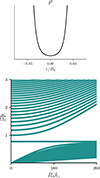Fig. 5. Dispersion relations of the global modes in a pressure minimum.

4.3. Gap in a disc

To test these predictions in a realistic gap in a disc, we studied the spectrum of an extended disc with power-law profiles (as discussed in Sect. 3.3) and a gap is carved. More precisely, the volume density is taken as

$$\begin{array}{c}\hfill \rho \propto r^{-p-s+\frac{q}{2}}\times (1-Aexp(-{(r-r_{\mathrm{gap}})}^2/2L_{\mathrm{gap}}^2)).\end{array}$$(43)

This profile is shown in Fig. 6 (top), with the position of the gap r_gap = 8 r₀, width of the gap L_gap = 0.2 r₀, and relative depth of the gap, A = 0.99.

Fig. 6. Same as Fig. 3 but for a disc with a gap and zoomed on lower frequencies. In a disc where a gap of density is present, one local minimum and one local maximum of density are found. Associated to these extrema, two topological modes are expected and found in the spectrum, one inertial and one acoustic respectively. Dashed red lines show ω = κ(r = rmin) and ω = cs(r = rmax)kz.

Interestingly, the addition of a gap in the disc causes the addition of two new extrema of density: a minimum and a maximum, separated by approximately half the gap width. Based on the analysis described in the sections above, we would expect to find two topological modes localised at these regions of the disc, trapped by the density extrema. Close to r_min (i.e. close to the center of the gap), we would expect an epicyclic mode with dispersion relation of ω = κ(r = r_min), along with an acoustic mode close to r_max with dispersion relation of ω = c_s(r = r_max)k_z.

The bottom panel of Fig. 6 presents the numerically obtained spectrum of the disc. As before, the colours indicate the average mode positions, with modes located inside the gap highlighted in pink. In addition to the inertial and acoustic branches already present in the monotonic disc, we observed a new set of inertial branches (low-frequency, pink) as well as a new set of acoustic branches (yellow). Moreover, the two branches of modes predicted by the topological analysis are also visible, with their dispersion relations overlaid as thin grey lines. An inertial branch appears at ω = κ(r = r_min), while an acoustic branch follows ω = c_s(r = r_max)k_z. Because these two modes occupy nearby regions in radius, they get hybridised when their frequencies align, leading to an avoided crossing near r₀k_z ∼ 0.8. The low-frequency pink branch is not incidental: it represents a mode trapped in the gap and corresponds to the topological epicyclic mode, as shown by its eigenfunctions (see Appendix C).

Therefore, the density extrema act as waveguides, trapping modes in the way described in the analytical models presented in Sects. 4.1 and 4.2. In addition to the two topological modes, new branches of inertial modes appeared in the spectrum at low frequency, trapped in the gap. New branches of acoustic modes appear with average position in the yellow region, as those are instead trapped between the gap and the outer boundary. In that case, it appears that the gap of the disc acts as a reflector for acoustic waves.

5. Discussion

By leveraging topological methods, our analysis characterises how large-scale modes behave in radially structured discs. Emphasis was put on the role that radial pressure and density gradients play on linear stable waves, encapsulated by the characteristic frequency, S. Using micro-local techniques, we show that these gradients modify the local dispersion relations by coupling acoustic and inertial waves and removing their frequency degeneracy. As such, S naturally acts as a cutoff frequency and offers a consistent way to account for gradient effects in local analyses. Topological arguments highlight the significance of points where S = 0, which carry topological charges (Chern numbers 𝒞 = ±1). These charges impose the emergence of modes with unique spectral properties; namely, branches that transit between r-modes and p-modes. While a monotonic disc hosts only one such branch, structured discs contain additional ones, as illustrated in Fig. 6. We emphasise the fact that the gapped-disc model presented in Sect. 4.3 is intended as an illustrative example of trapped modes; although it reproduces the expected topological modes at pressure extrema, it is not meant to be realistic or to remain stable against the Rossby wave instability (Lovelace et al. 1999).

The fundamental mode trapped at a pressure maximum propagates for all frequencies and is the sole mode to do so (see Fig. 4), making it capable of resonating with any temporal forcing, unlike modes with forbidden frequency domains. It is a vertical acoustic wave (see Figs. C.1 and C.2). By contrast, the fundamental mode associated with a pressure minimum (a gap) propagates only at the constant frequency, ω = κ (see Figs. 5, C.3, and C.4), and it is a horizontal, epicyclic wave. This unique property thereby allows for a propagation at arbitrary vertical phase velocities. Indeed, since $\frac{\omega }{k_z}=\frac{\kappa }{k_z}$ can take any value, this mode is unique among the modes in having an arbitrary vertical phase velocity. This is a necessary condition for resonating with any vertical dust flow involved in dust-settling instabilities, a class of resonant drag instabilities (e.g. Squire & Hopkins 2018; Zhuravlev 2019; Lehmann & Lin 2023; Paardekooper & Aly 2025). In the analytical model of Sect. 4.2, this mode has no vertical velocity and therefore does not couple to vertical flows a priori. However, we emphasise that this is a peculiarity of that model. In general, the mode does exhibit some vertical-velocity perturbation (see Appendix C): this topological mode may thus be coupled to vertical flows in settling-instability mechanisms. It would be worthwhile to further investigate its role at the outer edge of a planetary gap, where dust accumulates. The spectrum of a disc with a pressure bump instead of a pressure gap produces similar results (see Fig. C.5).

At low k_z (see Fig. C.3), this mode exhibits a very similar character to the trapped r-modes found in black hole accretion discs (Kato 2004, 2008; Ferreira & Ogilvie 2008; Dewberry et al. 2018). Only here the mode is confined by the epicyclic-acoustic frequency rather than by the maximum in the relativistic epicyclic frequency found in black hole discs. This leaves open the possibility that this mode could be excited to large amplitudes via a similar three-wave coupling mechanism (Kato 2004, 2008; Ferreira & Ogilvie 2008), where the r-mode is coupled to a global m = 1 deformation in such a way that it leads to growth in the r-mode amplitude. Candidates for such a global m = 1 deformation include remnant disc eccentricity left over from the disc formation process (Commerçon et al. 2024) or disc warping and eccentricity excited by an embedded planet (Lubow & Ogilvie 2001; Teyssandier & Ogilvie 2016).

The main limitations of the present study are the absence of vertical stratification and of any linear instability. The vertical stratification is sometimes separated from the radial problem by averaging vertically (e.g. Papaloizou & Pringle 1985 or Blaes et al. 2006); we instead chose to assume no stratification, so as to keep the notion of a vertical wavenumber, k_z. We note that our analytical solutions for the slender torus Eq. (35) matches those of Blaes et al. (2006). We refer to their Eq. (56) for their n set to ∞ and our k_z = 0.

We also note that Eq. (21) is analogous to the one found by Okazaki et al. 1987 (Eq. (4.4)) who studied vertical isothermal stratification and no radial stratification, with two expected differences: the addition of S² representing radial gradients in our case and the replacement of c_s²k_z² by n_zκ² in their case, where n_z is a positive integer counting the number of nodes in the profile of pressure perturbation given by the Hermite function of order of n_z. Thus, vertical isothermal stratification seems to be fully taken into account by discretising wavenumbers as c_sk_z = n_z^1/2κ. However, the results of Korycansky & Pringle (1995) suggest an interesting behavior of the modes with vertical stratification and no radial gradients (see their Fig. 1). Indeed, they show that a pair of fundamental p-modes with indices of n_z = 0, 1 have frequencies that connect inertial modes and acoustic modes, possibly performing a spectral flow. This suggests that, in a complementary way, vertical stratification imposes another set of topological properties and topological modes, regardless of radial gradients.

The analytical techniques and solutions found for modes of non-axisymmetric polytropic discs, whether slender (Papaloizou & Pringle 1985; Blaes 1985; Blaes et al. 2006) or thick (Blaes et al. 2007), provide the support to explore the topology of these waves rising from vertical inhomogeneity, and from azimuthal wavenumbers and (possibly) associated topological modes. Our goal in the present study is to provide a starting point for applying topological analysis to linear waves in discs, a framework whose predictive power can yield new insights into large-scale oscillations in inhomogeneous discs, with the perspective of establishing robust and possibly unique properties of large-scale modes falling out of Wentzel-Kramers-Brioullin approaches. This line of research is motivated by the anticipated potential of discoseismology in protoplanetary discs, facilitated by line-kinematic measurements from ALMA (e.g. Pinte et al. 2023; Teague et al. 2025). While this perspective is still far off, we expect that the spatial patterns of the eigenmodes may provide constraints on models; this is a key distinction from stellar pulsation studies. The employment of a topological analysis to study linear instabilities in discs requires further investigation, as it is a field of research less developed than topology of stable waves. In stellar context, these ideas have led to the unveiling of fast-growing large-scale modes of compressible convective instability (Leclerc et al. 2024a). Similar results could be expected in discs instabilities when accounting for the role of pressure gradients, as we have done in the present study.

6. Conclusion

Motivated by the foreseen potential of discoseismology in protoplanetary discs enabled by line–kinematic measurements from ALMA, we conducted a topological analysis of radial waves in unstratified astrophysical discs. Our main conclusions are:

1. Existence of robust topological modes: Global large-scale modes transiting between the inertial and the acoustic bands exist in discs. These modes find their roots in topological numbers and, as such, they qualify as topological modes. This special origin provides them with unique properties.

2. Epicyclic–acoustic frequency: The existence of topological modes in discs is associated with the cancellation of the epicyclic-acoustic frequency, S, given by Eq. (12), which gives the rate of momentum exchange between the inertial and acoustic bands. This is why monotonic-density discs support a single topological mode at their inner edge.

3. Role of pressure extrema: Pressure maxima and minima, acting as waveguides, generate additional topological modes because S = 0 at these locations. The associated topological branch is acoustic at pressure maxima and inertial at pressure minima, both having a unique specificity across the spectrum (any frequency or any phase velocity). Their distinct features make them appealing targets for future line-based discoseismology. Furthermore, they are potentially easier to detect as they are localised and their radial trapping would provide a direct measure of the pressure gradient of the bump or dip.

4. Micro-local framework: The micro-local analysis introduced here enables the study of local wave properties without using a shearing box, while preserving the Hermitian structure of the problem. This approach provides a powerful framework for studying linear modes in discs.

As noted in the discussion presented in this paper, we have focused on the midplane, ignoring the influence of vertical stratification for the moment. Simultaneously treating vertical and radial gradients requires a complementary study, which could reveal additional topological structures in the higher dimensional parameter space involved. A stepping stone towards more general results, and potentially towards discoseismology, is to study a dual simplified problem where radial gradients are neglected, while keeping vertical stratification. A study of the topological modes of this problem will be the subject of a future work.

Data availability

The scripts written and used for numerical calculations are accessible at https://github.com/ArmandLeclerc/radialStratifDisc.

Acknowledgments

AL was funded by Contrat Doctoral Spécifique Normaliens during this work. GL, EL and NP acknowledge funding from ERC CoG project PODCAST No 864965. AL acknowledges funding from ERC StG project Calcifer No 101165631. We used MATHEMATICA (Wolfram Research Inc, 2024).

References

Appendix A: Constant of motion

The evolution equation of the perturbations X(r, k_z, t) is

$$\begin{array}{c}\hfill i{\partial }_{t}X=\mathcal{H}X.\end{array}$$(A.1)

As ℋ is self-adjoint with respect to the inner product,

$$\begin{array}{c}\hfill ⟨X,Y⟩={\displaystyle \int \mathrm{d}}r{X}^{\top \ast }·Y,\end{array}$$(A.2)

where ⋅ is the matricial product, such that ⟨X, ℋY⟩=⟨ℋX, Y⟩ for boundary conditions with zero radial velocity. We then have

$$\begin{array}{cc}\hfill i{\partial }_t⟨X,X⟩& =⟨-i{\partial }_{t}X,X⟩+⟨X,i{\partial }_{t}X⟩,\hfill \end{array}$$(A.3)

$$\begin{array}{cc}\hfill & =-⟨\mathcal{H}X,X⟩+⟨X,\mathcal{H}X⟩,\hfill \end{array}$$(A.4)

$$\begin{array}{cc}\hfill & =-⟨X,\mathcal{H}X⟩+⟨X,\mathcal{H}X⟩,\hfill \end{array}$$(A.5)

$$\begin{array}{cc}\hfill & =0.\hfill \end{array}$$(A.6)

$I=\frac{1}{2}⟨X,X⟩$ is then a constant of motion, given by the self-adjointess of the evolution operator ℋ. Equation (15) gives it in dimensional form, where we see that it is the pseudo-energy of the wave, expressed as the sum of kinetic and pressure energy contributions.

Appendix B: Self-adjointness of ℋ

We show here that ℋ is self-adjoint on the Hilbert space, {X = (u_z u_r u_θ h^⊤, u_r(r₀) = u_r(r₁) = 0}, with respect to the canonical inner product, ⟨X₁, X₂⟩=∫drX₁^*X₂.

$$\begin{array}{cc}\hfill ⟨X_1,\mathcal{H}{X}_2⟩& ={\displaystyle \int \mathrm{d}}r(c_{\mathrm{s}}{k}_z(u_{z,1}^{\ast }{h}_2+h_1^{\ast }{u}_{z,2})+i\kappa (u_{\theta ,1}^{\ast }{u}_{r,2}-u_{r,1}^{\ast }{u}_{\theta ,2}))\hfill \end{array}$$(B.1)

$$\begin{array}{cc}\hfill & +{\displaystyle \int \mathrm{d}}r{u}_{r,1}^{\ast }(i{c}_{\mathrm{s}}{\partial }_r{h}_2+i\frac{c_{\mathrm{s}}^{\prime }}{2}{h}_2-iS{h}_2)+{\displaystyle \int \mathrm{d}}r{h}_1^{\ast }(i{c}_{\mathrm{s}}{\partial }_r{u}_{r,2}+i\frac{c_{\mathrm{s}}^{\prime }}{2}{u}_{r,2}+iS{u}_{r,2}),\hfill \\ \hfill & ={\displaystyle \int \mathrm{d}}r(c_{\mathrm{s}}{k}_z(u_{z,1}^{\ast }{h}_2+h_1^{\ast }{u}_{z,2})+i\kappa (u_{\theta ,1}^{\ast }{u}_{r,2}-u_{r,1}^{\ast }{u}_{\theta ,2}))\hfill \end{array}$$(B.2)

$$\begin{array}{cc}\hfill & +[i{c}_{\mathrm{s}}{u}_{r,1}^{\ast }{h}_2]-{\displaystyle \int \mathrm{d}}r(i{c}_{\mathrm{s}}{\partial }_r{u}_{r,1}^{\ast }+i\frac{c_{\mathrm{s}}^{\prime }}{2}{u}_{r,1}^{\ast }+iS{u}_{r,1}^{\ast })h_2+[i{c}_{\mathrm{s}}{h}_1^{\ast }{u}_{r,2}]-{\displaystyle \int \mathrm{d}}r(i{c}_{\mathrm{s}}{\partial }_r{h}_1^{\ast }+i\frac{c_{\mathrm{s}}^{\prime }}{2}{h}_1^{\ast }-iS{h}_1^{\ast })u_{r,2},\hfill \\ \hfill & ={\displaystyle \int \mathrm{d}}r({(c_{\mathrm{s}}{k}_z{u}_{z,1})}^{\ast }{h}_2+{(c_{\mathrm{s}}{k}_z{h}_1)}^{\ast }{u}_{z,2}+{(-i\kappa u_{\theta ,1})}^{\ast }{u}_{r,2}+{(i\kappa u_{r,1})}^{\ast }{u}_{\theta ,2}))\hfill \end{array}$$(B.3)

$$\begin{array}{cc}\hfill & +[i{c}_{\mathrm{s}}{u}_{r,1}^{\ast }{h}_2]+{\displaystyle \int \mathrm{d}}r{(i{c}_{\mathrm{s}}{\partial }_r{u}_{r,1}+i\frac{c_{\mathrm{s}}^{\prime }}{2}{u}_{r,1}+iS{u}_{r,1})}^{\ast }{h}_2+[i{c}_{\mathrm{s}}{h}_1^{\ast }{u}_{r,2}]+{\displaystyle \int \mathrm{d}}r{(i{c}_{\mathrm{s}}{\partial }_r{h}_1+i\frac{c_{\mathrm{s}}^{\prime }}{2}{h}_1-iS{h}_1)}^{\ast }{u}_{r,2},\hfill \\ \hfill & =⟨\mathcal{H}{X}_1,X_2⟩+[i{c}_{\mathrm{s}}(u_{r,1}^{\ast }{h}_2+h_1^{\ast }{u}_{r,2})].\hfill \end{array}$$(B.4)

The bracket term goes to zero for impenetrable boundaries and, therefore, ℋ is self-adjoint.

Appendix C: Profiles of modes

Fig. C.1. Relative amplitudes of the components of a fundamental p-mode with large kz, of topological origin, induced by a pressure bump located close to rmax. The amplitudes are displayed as functions of the distance to the central object in the mid-plane (top right panel) and for a (r,z) slice of the disc (bottom panel). The selected mode is marked with a cross in the top left panel (same as Fig. 3). This mode has an amplitude in uz and h and, as such, is of acoustic nature. Interestingly, it mixes with both the fundamental r-mode of the gap and an inertial mode of the inner disc, which both have amplitudes in ur and uθ. It is more spatially extended around rmax than the fundamental r-mode is around rmin (see below).

Fig. C.2. Same as Fig. C.1 but for a mode a low kz (note the different z scale). The properties of this mode are similar to the one displayed in Fig. C.1.

Fig. C.3. Same as Fig. C.1 but for the the fundamental r-mode, topologically induced by the existence of the a pressure gap. The mode exhibits strong horizontal motions around rmin (note the scale colour bars), where the amplitude peaks. The mode extends outwards of the gap, and has non-zero amplitude at rmax, where grains may eventually pile-up. The mode mixes with acoustic vibrations outside of rmin.

Fig. C.4. Same as Fig. C.3 but for larger values of kz (note the different scale on z). The fundamental vibration of the gap couples with an inertial vibration of the rest of the disc, such that vertical motions have comparable amplitudes with horizontal motions within the gap (note the scales colorbars).

Fig. C.5. Same as Fig. C.1 but for a disc with a pressure bump. The parameters of the bump are similar to the ones used to parametrise the gap, with a reversed amplitude A = −20. The mode is essentially of acoustic nature, while it mixes with inertial modes in the inner regions. The inertial topological mode associated with the presence of a pressure minimum at the inner edge is present, but difficult to distinguish since it is very de-localised.

All Figures

	Fig. 1. Local dispersion relation has a forbidden range of frequency when there is a non-zero value of S (i.e a non-zero pressure gradient), where no inertial nor acoustic wave propagates (shaded region).
In the text

	Fig. 2. Berry curvature, F, of the acoustic wave is singular at (cskr, S, cskz) = (0, 0, ±κ). This obstruction is a topological constraint, characterised by the two charges 𝒞 = ±1. Length and brightness of the arrows indicate the norm of F.
In the text

	Fig. 3. Global modes of a monotonic disc. The one topological branch transits from inertial modes (blue) at low kz to acoustic modes (yellow) at high kz. It matches the dispersion relation ω = cs(r0)kz (dashed red line).
In the text

	Fig. 4. Dispersion relations of the global modes in a slender torus.
In the text

	Fig. 5. Dispersion relations of the global modes in a pressure minimum.
In the text

	Fig. 6. Same as Fig. 3 but for a disc with a gap and zoomed on lower frequencies. In a disc where a gap of density is present, one local minimum and one local maximum of density are found. Associated to these extrema, two topological modes are expected and found in the spectrum, one inertial and one acoustic respectively. Dashed red lines show ω = κ(r = rmin) and ω = cs(r = rmax)kz.
In the text

Fig. C.1. Relative amplitudes of the components of a fundamental p-mode with large kz, of topological origin, induced by a pressure bump located close to rmax. The amplitudes are displayed as functions of the distance to the central object in the mid-plane (top right panel) and for a (r,z) slice of the disc (bottom panel). The selected mode is marked with a cross in the top left panel (same as Fig. 3). This mode has an amplitude in uz and h and, as such, is of acoustic nature. Interestingly, it mixes with both the fundamental r-mode of the gap and an inertial mode of the inner disc, which both have amplitudes in ur and uθ. It is more spatially extended around rmax than the fundamental r-mode is around rmin (see below).

In the text

	Fig. C.2. Same as Fig. C.1 but for a mode a low kz (note the different z scale). The properties of this mode are similar to the one displayed in Fig. C.1.
In the text

Fig. C.3. Same as Fig. C.1 but for the the fundamental r-mode, topologically induced by the existence of the a pressure gap. The mode exhibits strong horizontal motions around rmin (note the scale colour bars), where the amplitude peaks. The mode extends outwards of the gap, and has non-zero amplitude at rmax, where grains may eventually pile-up. The mode mixes with acoustic vibrations outside of rmin.

In the text

	Fig. C.4. Same as Fig. C.3 but for larger values of kz (note the different scale on z). The fundamental vibration of the gap couples with an inertial vibration of the rest of the disc, such that vertical motions have comparable amplitudes with horizontal motions within the gap (note the scales colorbars).
In the text

Fig. C.5. Same as Fig. C.1 but for a disc with a pressure bump. The parameters of the bump are similar to the ones used to parametrise the gap, with a reversed amplitude A = −20. The mode is essentially of acoustic nature, while it mixes with inertial modes in the inner regions. The inertial topological mode associated with the presence of a pressure minimum at the inner edge is present, but difficult to distinguish since it is very de-localised.

In the text

References

- Abramowitz, M., & Stegun, I. A. 1972, Handbook of Mathematical Functions (US Department of Commerce) [Google Scholar]
- Aerts, C., Christensen-Dalsgaard, J., & Kurtz, D. W. 2010, Asteroseismology (Springer Science+Business Media B.V.) [Google Scholar]
- Andrews, S. M., Huang, J., Pérez, L. M., et al. 2018, ApJ, 869, L41 [NASA ADS] [CrossRef] [Google Scholar]
- Armitage, P. J. 2011, ARA&A, 49, 195 [Google Scholar]
- Bae, J., Isella, A., Zhu, Z., et al. 2023, ASP Conf. Ser., 534, 423 [NASA ADS] [Google Scholar]
- Balbus, S. A., & Hawley, J. F. 1991, ApJ, 376, 214 [Google Scholar]
- Balbus, S. A., & Hawley, J. F. 1998, Rev. Mod. Phys., 70, 1 [Google Scholar]
- Blaes, O. 1985, MNRAS, 216, 553 [CrossRef] [Google Scholar]
- Blaes, O. M., Arras, P., & Fragile, P. 2006, MNRAS, 369, 1235 [NASA ADS] [CrossRef] [Google Scholar]
- Blaes, O. M., Šrámková, E., Abramowicz, M. A., Kluźniak, W., & Torkelsson, U. 2007, ApJ, 665, 642 [Google Scholar]
- Burns, K. J., Vasil, G. M., Oishi, J. S., Lecoanet, D., & Brown, B. P. 2020, PRR, 2, 023068 [Google Scholar]
- Commerçon, B., Lovascio, F., Lynch, E., & Ragusa, E. 2024, A&A, 689, L9 [NASA ADS] [CrossRef] [EDP Sciences] [Google Scholar]
- Delplace, P. 2022, SciPost Phys. Lecture Notes, 039 [Google Scholar]
- Delplace, P., Marston, J., & Venaille, A. 2017, Science, 358, 1075 [Google Scholar]
- Dewberry, J. W., Latter, H. N., & Ogilvie, G. I. 2018, MNRAS, 476, 4085 [Google Scholar]
- Dewberry, J. W., Latter, H. N., Ogilvie, G. I., & Fromang, S. 2020a, MNRAS, 497, 435 [Google Scholar]
- Dewberry, J. W., Latter, H. N., Ogilvie, G. I., & Fromang, S. 2020b, MNRAS, 497, 451 [NASA ADS] [CrossRef] [Google Scholar]
- Drażkowska, J., Bitsch, B., Lambrechts, M., et al. 2023, ASP Conf. Ser., 534, 717 [NASA ADS] [Google Scholar]
- Faure, F. 2023, Annales Henri Lebesgue, 6, 449 [Google Scholar]
- Ferreira, B. T., & Ogilvie, G. I. 2008, MNRAS, 386, 2297 [Google Scholar]
- Fuller, J. 2014, Icarus, 242, 283 [Google Scholar]
- Goldreich, P., & Lynden-Bell, D. 1965a, MNRAS, 130, 97 [NASA ADS] [CrossRef] [Google Scholar]
- Goldreich, P., & Lynden-Bell, D. 1965b, MNRAS, 130, 125 [Google Scholar]
- Goldreich, P., & Tremaine, S. 1978, ApJ, 222, 850 [NASA ADS] [CrossRef] [Google Scholar]
- Goldreich, P., & Tremaine, S. 1979, ApJ, 233, 857 [Google Scholar]
- Goldreich, P., & Tremaine, S. 1980, ApJ, 241, 425 [Google Scholar]
- Goodman, J. 1993, ApJ, 406, 596 [NASA ADS] [CrossRef] [Google Scholar]
- Hall, B. C. 2013, Quantum Theory for Mathematicians (Springer) [Google Scholar]
- Hedman, M., & Nicholson, P. 2013, AJ, 146, 12 [NASA ADS] [CrossRef] [Google Scholar]
- Hill, G. W. 1878, Am. J. Math., 1, 5 [Google Scholar]
- Iga, K. 2001, Fluid Dyn. Res., 28, 465 [Google Scholar]
- Johansen, A., Oishi, J. S., Low, M.-M. M., et al. 2007, Nature, 448, 1022 [NASA ADS] [CrossRef] [Google Scholar]
- Kato, S. 1978, MNRAS, 185, 629 [NASA ADS] [CrossRef] [Google Scholar]
- Kato, S. 1983, Astron. Soc. Japan, 35, 249 [Google Scholar]
- Kato, S. 2004, PASJ, 56, 905 [NASA ADS] [Google Scholar]
- Kato, S. 2008, PASJ, 60, 111 [NASA ADS] [Google Scholar]
- Kato, S. 2024, MNRAS, 528, 1408 [Google Scholar]
- Kato, S., & Fukue, J. 1980, PASJ, 32, 377 [NASA ADS] [Google Scholar]
- Keppeler, S. 2004, Introduction to Wigner-Weyl Calculus [Google Scholar]
- Korycansky, D. G., & Pringle, J. E. 1995, MNRAS, 272, 618 [Google Scholar]
- Latter, H. N., & Papaloizou, J. 2017, MNRAS, 472, 1432 [CrossRef] [Google Scholar]
- Le Saux, A., Leclerc, A., Laibe, G., Delplace, P., & Venaille, A. 2025, ApJ, 987, L12 [Google Scholar]
- Leclerc, A. 2025, Ph.D. Thesis, Ecole normale supérieure de Lyon, France [Google Scholar]
- Leclerc, A., Laibe, G., Delplace, P., Venaille, A., & Perez, N. 2022, ApJ, 940, 84 [Google Scholar]
- Leclerc, A., Jezequel, L., Perez, N., et al. 2024a, PRR, 6, L012055 [Google Scholar]
- Leclerc, A., Laibe, G., & Perez, N. 2024b, PRR, 6, 043299 [Google Scholar]
- Lehmann, M., & Lin, M.-K. 2023, MNRAS, 522, 5892 [CrossRef] [Google Scholar]
- Lesur, G., Flock, M., Ercolano, B., et al. 2023, ASP Conf. Ser., 534, 465 [NASA ADS] [Google Scholar]
- Lin, C. C., & Shu, F. H. 1966, Proc. Natl. Acad. Sci., 55, 229 [NASA ADS] [CrossRef] [Google Scholar]
- Lin, M.-K., & Youdin, A. N. 2015, ApJ, 811, 17 [NASA ADS] [CrossRef] [Google Scholar]
- Lindblad, B. 1948, MNRAS, 108, 214 [Google Scholar]
- Lovelace, R., Li, H., Colgate, S., & Nelson, A. 1999, ApJ, 513, 805 [NASA ADS] [CrossRef] [Google Scholar]
- Lubow, S. H., & Ogilvie, G. I. 1998, ApJ, 504, 983 [Google Scholar]
- Lubow, S. H., & Ogilvie, G. I. 2001, ApJ, 560, 997 [Google Scholar]
- Lubow, S. H., & Pringle, J. E. 1993, ApJ, 409, 360 [Google Scholar]
- Lynden-Bell, D., & Kalnajs, A. 1972, MNRAS, 157, 1 [NASA ADS] [CrossRef] [Google Scholar]
- Lynden-Bell, D., & Ostriker, J. P. 1967, MNRAS, 136, 293 [Google Scholar]
- Marley, M. S. 1991, Icarus, 94, 420 [Google Scholar]
- Nelson, R. P., Gressel, O., & Umurhan, O. M. 2013, MNRAS, 435, 2610 [Google Scholar]
- Ogilvie, G. 1998, MNRAS, 297, 291 [Google Scholar]
- Ogilvie, G. I., & Lubow, S. H. 1999, ApJ, 515, 767 [Google Scholar]
- Oishi, J. S., Burns, K. J., Clark, S. E., et al. 2021, J. Open Source Softw., 6, 3079 [Google Scholar]
- Okazaki, A. T., Kato, S., & Fukue, J. 1987, Publ. Astron. Soc. Japan, 39, 457 [NASA ADS] [Google Scholar]
- Onuki, Y. 2020, JFM, 883, A56 [Google Scholar]
- Ortega-Rodríguez, M., Solís-Sánchez, H., Álvarez-García, L., & Dodero-Rojas, E. 2020, MNRAS, 492, 1755 [Google Scholar]
- Paardekooper, S.-J., & Aly, H. 2025, A&A, 697, A40 [NASA ADS] [CrossRef] [EDP Sciences] [Google Scholar]
- Papaloizou, J., & Pringle, J. 1985, MNRAS, 213, 799 [Google Scholar]
- Parker, J. B., Marston, J., Tobias, S. M., & Zhu, Z. 2020, Phys. Rev. Lett., 124, 195001 [Google Scholar]
- Perez, N. 2022, Ph.D. Thesis, Ecole normale supérieure de Lyon, France [Google Scholar]
- Perez, N., Delplace, P., & Venaille, A. 2022, Phys. Rev. Lett., 128, 184501 [NASA ADS] [CrossRef] [Google Scholar]
- Perez, N., Leclerc, A., Laibe, G., & Delplace, P. 2025, JFM, 1003, A35 [Google Scholar]
- Perrot, M., Delplace, P., & Venaille, A. 2019, Nature Physics, 15, 781 [Google Scholar]
- Pinte, C., Teague, R., Flaherty, K., et al. 2023, ASP Conf. Ser., 534, 645 [NASA ADS] [Google Scholar]
- Qin, H., & Fu, Y. 2023, Sci. Adv., 9, 8041 [Google Scholar]
- Safronov, V. S. 1972, Evolution of the Protoplanetary Cloud and Formation of the Earth and Planets (Keter Publishing House) [Google Scholar]
- Solheim, J. E., Provencal, J. L., Bradley, P. A., et al. 1998, A&A, 332, 939 [Google Scholar]
- Squire, J., & Hopkins, P. F. 2018, MNRAS, 477, 5011 [Google Scholar]
- Teague, R., Benisty, M., Facchini, S., et al. 2025, ApJ, 984, L6 [Google Scholar]
- Teyssandier, J., & Ogilvie, G. I. 2016, MNRAS, 458, 3221 [NASA ADS] [CrossRef] [Google Scholar]
- Toomre, A. 1964, ApJ, 139, 1217 [Google Scholar]
- Tsang, D., & Butsky, I. 2013, MNRAS, 435, 749 [NASA ADS] [CrossRef] [Google Scholar]
- Tsang, D., & Lai, D. 2009, MNRAS, 393, 992 [NASA ADS] [CrossRef] [Google Scholar]
- van Capelleveen, R. F., Ginski, C., Kenworthy, M. A., et al. 2025, ApJ, 990, L8 [Google Scholar]
- Vidal, J., & de Verdiére, Y. C. 2024, arXiv eprints [arXiv:2402.10749] [Google Scholar]
- Volovik, G. E. 2003, The Universe in a Helium Droplet (OUP Oxford), 117 [Google Scholar]
- Wolfram Research Inc. 2024, Mathematica, Version 14.0, Champaign, IL [Google Scholar]
- Youdin, A. N., & Goodman, J. 2005, ApJ, 620, 459 [Google Scholar]
- Zhuravlev, V. V. 2019, MNRAS, 489, 3850 [NASA ADS] [Google Scholar]