| Issue |
A&A
Volume 708, April 2026
|
|
|---|---|---|
| Article Number | A276 | |
| Number of page(s) | 9 | |
| Section | Interstellar and circumstellar matter | |
| DOI | https://doi.org/10.1051/0004-6361/202558419 | |
| Published online | 20 April 2026 | |
A new wideband radio polarization observation of the supernova remnant G315.4–2.3
1
School of Physics and Astronomy, Yunnan University,
Kunming
650500,
PR China
2
SKA Observatory, SKA-Low Science Operations Centre,
26 Dick Perry Avenue,
Kensington,
WA
6151,
Australia
3
Department of Astronomy and Astrophysics, University of California, Santa Cruz,
1156 High Street,
Santa Cruz,
CA
95064,
USA
4
Dunlap Institute for Astronomy and Astrophysics, University of Toronto,
50 St. George Street,
Toronto,
ON
M5S 3H4,
Canada
5
David A. Dunlap Department of Astronomy and Astrophysics, University of Toronto,
50 St. George Street,
Toronto,
ON
M5S 3H4,
Canada
6
Center for Astrophysics | Harvard & Smithsonian,
60 Garden Street,
Cambridge,
MA
02138,
USA
7
Dominion Radio Astrophysical Observatory, Herzberg Astronomy & Astrophysics, National Research Council Canada,
PO Box 248,
Penticton,
BC
V2A 6J9,
Canada
★ Corresponding authors: This email address is being protected from spambots. You need JavaScript enabled to view it.
; This email address is being protected from spambots. You need JavaScript enabled to view it.
Received:
5
December
2025
Accepted:
1
March
2026
Abstract
Context. The supernova remnant (SNR) G315.4-2.3 (MSH 14-63 or RCW 86) exhibits strong emission across the electromagnetic spectrum. Radio polarization observations probe magnetic fields and help us understand the evolution of the SNR.
Aims. We investigated the radio spectrum and magnetic field properties of the SNR.
Methods. We observed G315.4-2.3 using the Australia Telescope Compact Array (ATCA), covering the frequency range 1.1-3.1 GHz. We then performed rotation measure (RM) synthesis on the frequency cubes of Q and U to obtain the polarized intensity and RM. The regular component of the line-of-sight magnetic field was estimated from RM. The fractional polarization versus wavelength squared was used to constrain the properties of the turbulent magnetic field.
Results. We obtained image cubes of Stokes 1, Q, and U over the frequency range 1.319-3.023 GHz after excluding channels affected by radio frequency interference, images of polarized intensity P and RM, and images of fractional polarization p. The rms noise is 0.6 mJy beam−1 for the band-averaged I and is 90 μJy beam−1 for P. All images have been smoothed to a common resolution of 62″ × 33″. The comparison with single-dish observations indicates that our images have retained the larger-scale emission. We obtained a spectral index of α = −0.60 ± 0.03 for the SNR. The radio spectra are very similar for different areas of the SNR. The foreground RM was estimated to be approximately 55 rad m−2, and the internal RM of most SNR areas is small, less than about 50 rad m−2. The regular magnetic field along the line of sight was estimated to be about 1.4 μG in the southwest, much smaller than the total magnetic field. For most parts of the southwest and northeast, p is less than 8% and is nearly constant with λ2. We estimated the ratio of turbulent to regular magnetic field to be higher than about 3. The scale of the turbulent magnetic field for some areas in the northeast might be smaller than about 0.4 pc.
Conclusions. The radio characteristics, including the spectrum and turbulent magnetic field, are very similar in the northeast and southwest, even though the evolution is quite different for these two regions based on the current models. These should be taken into account for future modeling of the evolution of the SNR.
Key words: acceleration of particles / polarization / ISM: magnetic fields / ISM: supernova remnants / radio continuum: general
© The Authors 2026
 Open Access article, published by EDP Sciences, under the terms of the Creative Commons Attribution License (https://creativecommons.org/licenses/by/4.0), which permits unrestricted use, distribution, and reproduction in any medium, provided the original work is properly cited.
This article is published in open access under the Subscribe to Open model. This email address is being protected from spambots. You need JavaScript enabled to view it. to support open access publication.
1 Introduction
The object G315.4-2.3 was first identified as a supernova remnant (SNR) by Hill (1967) due to its nonthermal and polarized emission. It is also referred to as MSH 14-63 as it was cataloged by Mills et al. (1961) or RCW 86 (Rodgers et al. 1960), which is the bright optical nebula located in the southwest region of the source.
G315.4-2.3 is a very interesting SNR. It shows strong emission over almost the full electromagnetic spectrum, from TeV γ-ray (H. E. S. S. Collaboration 2018), GeV γ-ray (Yuan et al. 2014), X-ray (Bamba et al. 2023; Suzuki et al. 2022; Tsubone et al. 2017; Borkowski et al. 2001), optical (Smith 1997), and infrared (Williams et al. 2011) to radio (Dickel et al. 2001) bands. The origin of the TeV γ-ray emission remains uncertain; hadronic (Sano et al. 2019) and leptonic (Ajello et al. 2016) scenarios have been proposed. X-ray emission contains thermal and nonthermal components toward the northeast, northwest, and southwest parts of the SNR (Rho et al. 2002; Vink et al. 2006; Yamaguchi et al. 2008; Castro et al. 2013; Tsubone et al. 2017). The nonthermal X-ray emission requires electrons of TeV energy, which can only be accelerated with a high shock velocity. Toward the northeast, the shock velocity was measured to be 3000 km s−1 (Yamaguchi et al. 2016) to 6000 km s−1 (Helder et al. 2009). However, the shock velocity toward the southwest is much lower and only in the range 300-2000 km s−1 (Suzuki et al. 2022). The way in which the electrons are accelerated there with such a low shock velocity is puzzling. What is even more puzzling is the circular shape of the SNR from radio to X-ray bands, given that the shock velocities differ significantly between the northeast and southwest.
G315.4-2.3 is also an interesting target, thanks to its connection with the SN AD 185 in Chinese ancient records (Clark & Stephenson 1975), as such connections are very rare. This puts its age to be 1840 yr. Observations such as nonradiative Hα filaments (Smith 1997), Fe-rich ejecta (Rho et al. 2002; Ueno et al. 2007; Yamaguchi et al. 2008; Broersen et al. 2014), and the non-detection of any associated neutron star (Kaplan et al. 2004) indicate that G315.4-2.3 is a remnant of Ia SN. Williams et al. (2011) and Broersen et al. (2014) conducted hydrodynamic simulations showing that a Ia SN inside a cavity formed by the progenitor system can reproduce the multiwavelength SNR morphology and the high-energy γ-ray emission. In this scenario, due to either an off-center explosion or an inhomogeneous interstellar medium density, the northeast part encountered the cavity wall only recently, and the southwest started to interact with the wall about 300 yr after the explosion. This scenario provides an explanation for the difference in the shock velocities in the two regions. Alternatively, Gvaramadze et al. (2017) claimed the identification of a solar-type star in a binary system with a companion neutron star, and thus suggested that G315.4-2.3 is from a core-collapse SN. However, earlier observations by Mignani et al. (2012) had ruled out the companion as a neutron star. Therefore, the Ia SN scenario is more favored than the core-collapse SN scenario.
Radio polarization observations provide information on the spectrum and magnetic field, which helps us understand the emission and evolution of the SNR. However, there have only been a few polarization observations of G315.4-2.3 to date. Earlier observations were conducted with the Parkes 64 m telescope. Milne & Dickel (1975) observed the SNR at 5 GHz with a resolution of 4′.4 and detected strong polarized emission toward the east and southwest regions. The fractional polarization was about 5% and the magnetic field was approximately in the radial direction. Dickel & Milne (1976) observed the SNR at 2.7 GHz with a resolution of 8′.4 and found that the fractional polarization is very similar to that at 5 GHz toward the east and southwest regions.
Observations with an interferometer provide a higher-resolution image of the SNR. The SNR was observed by Dickel et al. (2001) with the Australian Telescope Compact Array (ATCA) at 1.34 GHz with a resolution of 8″, and polarized emission was detected at a few spots toward the east and southwest regions. Based on the six 32 MHz bands, an average Faraday rotation measure (RM) of about 60 rad m−2 was obtained. At a similar resolution, but with a much broader bandwidth covering the frequency range 856-1712 MHz, Cotton et al. (2024) observed the SNR with MeerKAT. They found very similar features in total intensity, but with a much higher sensitivity and dynamic range than that observed by Dickel et al. (2001). They also detected more polarized emission, and thus obtained RMs for almost the entire SNR shell. The RM values are consistent with those of Dickel et al. (2001).
In this paper, we report a new wideband polarization observation of G315.4-2.3, conducted with the ATCA, covering the frequency range 1.1-3.1 GHz, which bridges the frequency gap of the observations currently available. The paper is organized as follows: the observations and data reduction are presented in Sect. 2; the results are shown in Sect. 3; the discussions are presented in Sect. 4; and our conclusions are drawn in Sect. 5.
2 Observations and data reduction
We observed G315.4-2.3 with the ATCA (Project ID: C3246) using the Compact Array Broad-band Backend (CABB, Wilson et al. 2011). The observations covered the frequency range 1.1-3.1 GHz split into 2048 1 MHz channels. Since G315.4-2.3 has an angular size that is much larger than the primary beam, the mosaicking mode was used for the observations. In total, 43 pointings were observed to achieve full spatial Nyquist sampling up to 3.1 GHz. To achieve good uv coverage, six array configurations were used, H75, H168, EW352, 750C, 1.5A, and 1.5D, with baselines ranging from 30.6 m to about 1.5 km. The observations were conducted seven times from April to September 2018. The total integration time was ~0.4 h per pointing.
Calibration and imaging were performed using MIRIAD (Sault et al. 1995). Bandpass solutions were derived from 1934-63 8 or 0823-500. Gain and polarization leakage were solved for using the phase calibrator 1352-63; the observations spanned a wide range of parallactic angles. The phase calibrator was observed approximately every 16 minutes, and gain solutions were derived over the same time interval. Observations of the targets were bracketed by observations of the phase calibrator, and the phase solution was interpreted between observations of the calibrator. To account for the frequency-dependent variation of the gains, we split the 2 GHz bandwidth into eight subbands to derive the solutions separately. These solutions were scaled to match the flux density model of 1934-638 and then applied to the targets before imaging.
Our observations were also influenced by radio frequency interference (RFI); strong RFI was always present, especially at the low-frequency end of the band. After flagging, approximately 40% of the data were discarded and all data at 1.1-1.3 GHz were flagged.
We imaged Stokes I, Q, and U by joint deconvolution of all the pointings every 16 consecutive channels, using the MIRIAD tasks MOSMEM and PMOSMEM. The Briggs weighting (Briggs 1995) with robust = −1 was used. The uv-coverage for the 16 channels centered at the high-frequency end of 3.023 GHz is shown in Fig. 1, where the minimum uv distance is about 0.2 kλ, corresponding to a maximum angular scale of approximately 17′.
We obtained 80 images of I, Q, and U using 16 MHz bandwidth each, ranging from 1.319 GHz to 3.023 GHz. We smoothed the resultant images to a common resolution of 62″ × 33″. For I, we averaged all the channels to obtain the image centered at 2.2 GHz. For Q and U, we applied RM synthesis (Brentjens & de Bruyn 2005) to obtain the polarized intensity and RM.
According to Burn (1966), the following Fourier transform relation holds:  , where P is the observed complex polarized intensity and its absolute value is the polarized intensity;
  is the Faraday depth, K is a constant, ne is the thermal electron density, B|| is the line-of-sight component of the magnetic field, and the integral is along the line of sight from a position r in the source to the observer; F(φ) is the Faraday spectrum with the absolute value |F(φ)| representing polarized intensity as a function of Faraday depth φ. For polarized emission, |F(φ)| peaks at the RM of the emission with the peak value corresponding to the polarized intensity (P).
Rotation measure synthesis derives F(φ) from the observed P(λ2) using the Fourier transform. Due to the limited bandwidth, P is not fully sampled, and correspondingly there is an RM spread function (RMSF) in the Faraday depth domain. The full width at half maximum (FWHM) of the RMSF contributes to the uncertainty of RM. For details on RM synthesis and calculation of the FWHM of the RMSF, we refer to Brentjens & de Bruyn (2005).
We used RM-Tools (Purcell et al. 2020) to perform RM synthesis and then searched for the peaks in |F(φ)| to derive RM and P. The intrinsic polarization angle (χ0) after correction for the Faraday rotation with the derived RM was also obtained.
The bandwidth of the previous ATCA observations of G315.4-2.3 by Dickel et al. (2001) is too narrow, and the frequency band has been covered by our new observations. The MeerKAT observations missed large-scale emission, as shown in Sect. 3.1. We thus did not include these two observations when performing the RM synthesis and fractional polarization analysis.
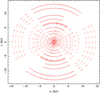 |
Fig. 1 uv coverage of the 16 frequency channels centered at 3.023 GHz from all the pointings of G315.4-2.3. |
 |
Fig. 2 Total intensity (I) image and contours of G315.4-2.3 at 2.2 GHz from averaging all the frequency channels. The contour levels are at 20.5n × 5σI, n = 0,1,2,... The rms noise is σI = 0.6 mJy beam−1. The resolution is 62″ × 33″. The red dashed lines mark the four regions for which the spectral indices were derived and are shown in Fig. 4. |
3 Results
3.1 Total intensity and spectral index
The total intensity (I) image of G315.4-2.3 at 2.2 GHz is shown in Fig. 2, which has a resolution of 62″ × 33″ with a position angle (PA) of 84°. The rms noise is σI = 0.6 mJy beam−1. It shows an obvious circular shell-like structure with the two brightest segments toward the northeast and southwest, similar to the radio images of Dickel et al. (2001) and Cotton et al. (2024). It also resembles the X-ray (Tsubone et al. 2017; Vink et al. 2006; Borkowski et al. 2001) and optical (Smith 1997) images.
We measured an integrated flux density of 21.7±1.1 Jy at 2.2 GHz from Fig. 2. We also collected previously published flux density values or measured flux density from the available surveys. The integrated flux density Sν and the frequency ν are listed in Table 1. We also measured the integrated flux density from all the 80 ATCA images. The uncertainties of the measurements include a conservative 5% calibration error (Butler et al. 2018). All the flux densities (Sν) versus frequencies (ν) are shown in Fig. 3.
The new measurements of integrated flux density are consistent with those from single-dish observations by Murriyang at 1.41, 2.4, and 2.65 GHz, indicating that the missing flux density with ATCA is negligible across the entire band. This is the result expected from the joint deconvolution that delivers a maximum angular scale of λ/(dmin - D/2), where dmin is the minimum baseline and D = 22 m is the diameter of the ATCA telescope (e.g., McClure-Griffiths et al. 2001). Even at the high-frequency end of 3.023 GHz with dmin = 0.2 kλ (Fig. 1), the maximum angular scale is about 38′, roughly the size of G315.4-2.3. Therefore, all the flux can be recovered.
We fit the integrated flux density versus frequency to a power law, Sν ∝ να, and obtained the spectral index α = −0.60 ± 0.03. This is consistent with α = −0.62 obtained by Caswell et al. (1975) based on the measurements at 85.5, 1410, and 2650 MHz, although their values are larger than our fit shown in Fig. 3.
Several measurements deviate from the fitting, as can be seen in Fig. 3. The integrated flux densities at 408 MHz and 5000 MHz (Caswell et al. 1975) are larger than the fitting, but have large uncertainties (Table 1), and the maps were too small in angular size to accurately subtract background emission. The three measurements at 843 MHz by MOST, at 1335 MHz by MeerKAT, and at 4850 MHz by Murriyang all miss flux density of large-scale emission and fall below the fitted line. For MOST, there was a lack of baselines shorter than 15 m, which made the observations insensitive to structures on scales larger than ~30′ (Whiteoak & Green 1996). For the MeerKAT observation, the imaging used an inner Gaussian taper, which reduced sensitivity to large-scale emission (Cotton et al. 2024). For the Murriyang observation, the data processing employed a 57' running-median baseline subtraction, which suppressed structures with angular scales larger than ~30′ (Condon et al. 1993).
To investigate spatial variations, the remnant was divided into four regions outlined in Fig. 2. The integrated flux densities were derived for each individual region and for all 80 channels. The spectral index was also obtained by fitting the data to a power law. The results are shown in Fig. 4. Taking into account the uncertainties, the difference among the spectral indices is small.
Integrated flux density of SNR G315.4-2.3.
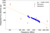 |
Fig. 3 Integrated flux density vs. frequency for SNR G315.4-2.3. The blue points were measured from the 80 I images; the red points are from Table 1. |
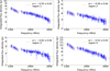 |
Fig. 4 Same as Fig. 3, but for the four regions marked in Fig. 2 and showing only the new measurements from ATCA. |
3.2 Polarized intensity and RM
We obtained a cube of Faraday depth from −500 to +500 rad m−2 in steps of 5 rad m−2, and images of ϕpeak, |F (ϕpeak)|, and intrinsic polarization angle χ0 from RM synthesis. For |φ| close to 500 rad m−2, the frames in the cube contain predominantly noise; we measured from these frames an rms noise of σP = 90 μJy beam−1 for polarized intensity. We set a threshold of |F(ϕpeak)| > 8σP, which means the RM uncertainty is better than FWHM/2(P/σP) ≈ 5 rad m−2. Here, FWHM ≈ 83 rad m−2 determined by the maximum separation of λ2 of the 80 frequency channels (Brentjens & de Bruyn 2005), and P/σP is the signal-to-noise ratio for P.
We show |F (ϕpeak)| in Fig. 5 and ϕpeak in Fig. 6. The orientation of the magnetic field (χ0 + 90°) is also depicted in Fig. 5. The Faraday spectra for pixels from different parts of the SNR covering a wide range of ϕpeak values were extracted from the cube and are shown in Fig. A.1. These spectra exhibit simple profiles with a single dominant peak, and thus ϕpeak and |F(ϕpeak)| correspond to RM and P, respectively. We note that with the large FWHM of the RMSF, simple profiles could hide the complexity that may be present. The complexity occurs when there is a mixture of synchrotron-emitting and Faraday-rotating medium or there are multiple emitting components, each with a different Faraday depth (e.g., Sun et al. 2015). The complexity leads to wavelength-dependent depolarization (Sokoloff et al. 1998), which was not observed, as shown later. This supports that the spectra are simple.
We detected polarized emission from most of the shell of G315.4-2.3. The strongest polarized intensity appears in the southwest, where the magnetic field appears to be perpendicular to the shell. This was also observed by Dickel et al. (2001) with ATCA and Cotton et al. (2024) with MeerKAT. In addition to the southwest, the previous ATCA observation only detected polarized emission from a few spots in the northeast (Dickel et al. 2001); the MeerKAT observation also detected polarized emission from most of the SNR revealing much finer details (Cotton et al. 2024).
The RM shows a large variation across the SNR. Toward the southwest the RM is around 80 rad m−2; toward the northeast the RM decreases from about 70 rad m−2 in the lower part to about 45 rad m−2 in the upper part; toward the northwest the RM is the largest and around 90 rad m−2. The narrower band of the previous ATCA observation (Dickel et al. 2001) does not allow for a reliable estimate of RM. The RM image from MeerKAT (Cotton et al. 2024) is strikingly consistent with ours, but with finer details. This might imply that missing flux in total intensity does not influence the RM determination (e.g., Ordog et al. 2025).
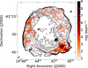 |
Fig. 5 Image of |F(φpeak)|, corresponding to polarized intensity P, superimposed with I contours of G315.4-2.3. The contour levels are the same as in Fig. 2. The bars indicate the orientation of magnetic fields with lengths proportional to P. |
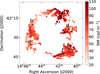 |
Fig. 6 RM (ϕpeak) image of G315.4-2.3. For the pixels labeled a-f, the Faraday spectra were extracted from the cube and are shown in Fig. A.1. |
3.3 Fractional polarization
The fractional polarization can be derived as p = P/I. We note that the polarized intensity from RM synthesis is at λ0, which is the average of λ2 of all channels (Brentjens & de Bruyn 2005). In our case, λ0 corresponds to the frequency of 2.02 GHz. We scaled I from 2.2 GHz (Fig. 2) to 2.02 GHz using the spectral index of −0.6 (Fig. 3). We also set thresholds of I > 5σI, P > 8σP, and  . The image of p is shown in Fig. 7.
Toward the northeast and southwest there are mixed regions of low (p ≈ 3%) and high (p ≈ 15%) fractional polarization; toward the northwest the fractional polarization is mostly high at a level greater than about 11%. The median fractional polarization is ~9% for the entire SNR.
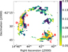 |
Fig. 7 Fractional polarization (p) of G315.4-2.3 at 2.02 GHz. Several regions are outlined for analysis shown in Fig. 9. |
4 Discussions
We adopted a distance d = 2.5 kpc for G315.4-2.3, which is commonly referenced in the literature (e.g., Broersen et al. 2014). Published measurements give d = 2.3 kpc from Balmer-dominated filament VLSR kinematics (Sollerman et al. 2003) and d = 2.8 kpc from optical/H I kinematics (Rosado et al. 1996). We therefore adopt d = 2.5 kpc as a representative midpoint.
4.1 Foreground RM
The RMs shown in Fig. 6 contain contributions from the Galactic foreground and the SNR itself, and it is necessary to separate them. We searched for pulsars from the ATNF pulsar catalog (Manchester et al. 2005, version 2.6.5) within a 5° radius centered at G315.4-2.3, and plotted RM and dispersion measure (DM) versus distance in Fig. 8.
The RMs appear to increase until a distance of about 2 kpc, reaching a value of about 55 rad m−2 , and then show a large scatter beyond the distance of about 2.5 kpc; the DMs generally increase linearly, but the slope is nearly flat between 2 and 3 kpc. Consequently, we assume that the increase in RM between 2 and 3 kpc is also small, and we take the value of 55 rad m−2 as the foreground. Unfortunately, there are only three pulsars in front of the SNR, and the estimate of foreground RM is very uncertain.
For a larger foreground RM, we would expect the average RMs of pulsars beyond 2 kpc to be systematically larger. Although this does not seem to be the case, as can be seen in Fig. 8, this cannot be ruled out because of the small number of pulsars.
For a much smaller foreground RM, the internal RM would be large, causing Faraday differential depolarization (Sokoloff et al. 1998). However, the spatial pattern of the fractional polarization (Fig. 7) does not follow that of the RM (Fig. 6), particularly for the northwest where the fractional polarization is higher, but the RM is also larger than the rest of the SNR. Assuming that the depolarization was primarily due to internal RM, the opposite would be expected since a larger RM results in a larger depolarization, and hence a lower fractional polarization. Therefore, a much smaller foreground RM is not favored.
There is depolarization caused by the internal RM only in areas with large RMs around 100 rad m−2. The internal RM contributed by the SNR can reach about 50 rad m−2 toward the northwest after subtracting the foreground RM. If we suppose a uniform mixture of thermal and relativistic electrons, the observed fractional polarization is expected to be pobs = pi sin(2RMλ2)/(2RMλ2), where pi is the intrinsic fractional polarization (Sokoloff et al. 1998). For pi ≈ 70% and RM = 50 rad m−2, pobs is about 25% at 2.02 GHz, larger than the observed values toward the northwest (Fig. 7), implying that there is further depolarization.
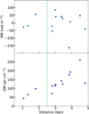 |
Fig. 8 RM and DM vs. distance for pulsars within 5° of G315.4-2.3 center. The green dashed line indicates the distance of 2.5 kpc. |
4.2 Magnetic field in the southwest
The magnetic field can be estimated on the basis of RM provided with the thermal electron density. The thermal electron density can be derived from the Hα observations. We used the Hα image compiled by Finkbeiner (2003). There is only strong Hα emission toward the southwest, where we can estimate the magnetic field.
The emission measure (EM) can be derived as ![Mathematical equation: ${\rm EM}=2.75T_4^{0.9}I_{\rm H\alpha}\exp[2.44E(B-V)]$](/articles/aa/full_html/2026/04/aa58419-25/aa58419-25-eq4.png) (Haffner et al. 1998), where T4 is the electron temperature in 104 K, IHα is the Hα intensity in Rayleigh, E(B - V) is the color excess, and EM is in pc cm −6. Toward the southwest, we obtained EM ≈ 443 pc cm−6 with background-subtracted IHα = 54 Rayleigh from the Hα map (Finkbeiner 2003), E(B - V) = 0.53 from the 3D extinction map (Chen et al. 2019), and T4 = 0.8 (Reynolds 1985).
(Haffner et al. 1998), where T4 is the electron temperature in 104 K, IHα is the Hα intensity in Rayleigh, E(B - V) is the color excess, and EM is in pc cm −6. Toward the southwest, we obtained EM ≈ 443 pc cm−6 with background-subtracted IHα = 54 Rayleigh from the Hα map (Finkbeiner 2003), E(B - V) = 0.53 from the 3D extinction map (Chen et al. 2019), and T4 = 0.8 (Reynolds 1985).
We assumed that the path length L is the same as the width of the shell, which is about 6′ corresponding to 4.4 pc with d = 2.5 kpc. The electron density was then estimated to be  cm−3 with a filling factor of 1, and the line-of-sight component of the magnetic field was estimated to be B|| ≈ R/0.81 neL ≈ 1.4 μG. Here R = 2RM is the full RM and is twice the measured RM with thermal and nonthermal gas uniformly mixed (Sokoloff et al. 1998), and RM ≈ 25 rad m−2 after excluding the foreground contribution. The B|| derived this way represents the regular component alone.
The fitting of the spectral energy distribution of synchrotron emission including observations from radio, X-rays, and γ-rays by Ajello et al. (2016) yielded a transverse magnetic field of 16.8 ± 2.1 μG for the southwest region. Toward the Galactic longitude of about 315° for a distance of 2.5 kpc, RM is mainly contributed by the Carina arm, and the line-of-sight component is approximately at the same level as the transverse component, assuming that the magnetic field follows the spiral arm (Han et al. 2018, their Fig. 4). This means that the total magnetic field is much larger than the regular field along line of sight.
The regular B|| would become even smaller if the foreground RM were larger. In contrast, a smaller foreground RM would result in a larger regular B|| . For example, a foreground RM of one-half the currently used value can increase the regular B|| by a factor of 2, but a much smaller foreground RM introduces a larger depolarization that is not consistent with the observation. With a smaller filling factor of 0.1, the regular B|| increases by a factor ~3. Combining these together, the regular B|| is still smaller than the total magnetic field, implying the presence of a strong turbulent magnetic field.
Based on X-ray spectral analysis, Suzuki et al. (2022) found that there is highly amplified magnetic turbulence toward the southwest. This is consistent with our results.
4.3 Southwest versus northeast
The shock velocity of the southwest (Suzuki et al. 2022) is much smaller than that of the northeast (Helder et al. 2009; Yamaguchi et al. 2016), but the SNR retains a circular shape in radio and X-ray. The current models have suggested that the southwest interacted with a cavity wall shortly after the supernova explosion, and thus decelerated, whereas the northeast just started to interact with the wall (Williams et al. 2011; Broersen et al. 2014). It is worthwhile to compare the radio characteristics of these two regions.
4.3.1 Spectrum
There is no large spatial variation of the spectral index in the SNR, ranging from −0.5 to −0.6. A leptonic model can fit the broadband emission from radio to TeV X-ray well and yielded the spectral index of electrons Γe = 2.3 ± 0.1 (H. E. S. S. Collaboration 2018), corresponding to α = −(Γe −1)/2 = −0.65 ± 0.05. Fitting the broadband emission of the southwest and northeast separately with a leptonic model yielded the same Γe = 2.21 ± 0.1 for both regions (Ajello et al. 2016), corresponding to α = −0.61 ± 0.05. This value is slightly steeper than the value we obtained: α = −0.55 ± 0.03 for the northeast (Fig. 4: region 1) and α = −0.52 ± 0.03 for the southwest (Fig. 4: region 4). The radio spectral indices for these two regions are also nearly the same.
Based on the current models, the southwest mainly contains an old population of electrons since the shock has long decelerated, and the northeast contains both old and young populations of electrons. Thus, it is expected that the spectrum of the southwest is steeper than that of the northeast because of synchrotron cooling. Spectral analysis of X-ray emission by Tsubone et al. (2017) showed that the power-law spectral index of the southwest is larger than that of the northeast. Unfortunately, radio emission at GHz is typically from GeV electrons that have a large cooling time on the order of 106 yr for a magnetic field of 20 μG as inferred from the fitting of broadband emission. Since the cooling time is much longer than the age of the SNR, the same radio spectra for the northeast and southwest support that the injected spectra of electrons accelerated by the SNR shocks are the same.
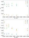 |
Fig. 9 Fractional polarization (p) vs. wavelength squared (λ2) for selected regions of southwest (upper panel) and northeast (lower panel). The regions are outlined in Fig. 7. |
4.3.2 Turbulent magnetic field
An enhanced turbulent magnetic field is required to accelerate electrons in SNR shocks (e.g., Bell 2004). In Sect. 4.2, we show that there is a strong turbulent magnetic field in the southwest. Magnetic field fluctuation causes depolarization (Sokoloff et al. 1998). Therefore, fractional polarization can help constrain the turbulent magnetic field.
We selected three regions that show different fractional polarizations (Fig. 7) from the northeast and southwest, respectively. We averaged Q, U, and I into six frequency bins from the 80 channel images to increase the signal-to-noise ratio. For each frequency bin, we used the RM of the SNR (Fig. 6) to derotate Q and U to the intrinsic polarization angle before averaging to account for bandwidth depolarization. We then averaged Q, U, and I for the six regions A-F and derived P, I, and p. In Fig. 9, we show the resulting p versus λ2.
For the southwest, p does not vary with λ2 for the three regions A-C (Fig. 9, upper panel). This indicates that there is little Faraday differential depolarization caused by internal RM. This also agrees with our foreground RM estimate, which results in a small internal RM. The low p is therefore probably caused by the magnetic field fluctuation. According to Sokoloff et al. (1998),  , where B⊥,reg is the regular transverse magnetic field and δB⊥ is the turbulent component. Here, the turbulent magnetic field is assumed to be isotropic. Therefore, the ratio of the turbulent to the regular component of the magnetic field can be estimated as
  . For pi = 0.7 and pobs ≈ 0.08 for regions A and C, the ratio is about 3, which agrees with the estimate for the line-of-sight magnetic field estimated in Sect. 4.2 taking into account the uncertainties of the foreground RM and the filling factor. For region B, the ratio is even higher.
For the northeast, p is also nearly constant with λ2 for regions D and F, similar to the southwest. The turbulent-to-regular ratio of the magnetic field of region F is similar to that of regions A and C in the southwest. For region E, p decreases from ~0.12 at λ2 ≈ 0.012 m2 to ~0.06 at λ2 ≈ 0.028 m2 and keeps roughly the same value until λ2 ≈ 0.045 m2. The average internal RM of region E is about 15 rad m−2 after excluding the foreground RM, which cannot account for the factor of 2 decrease in p with Faraday differential depolarization. With an RM scattering of σRM ≈ 20 rad m−2, the beam depolarization (Sokoloff et al. 1998) can produce the p decrease of about 50%, but will result in a much smaller p at the longest λ2 of about 0.045 m2. It could be that there are multiple emission components along the line of sight. At shorter wavelengths, all the components can be observed; at the long-wavelength end, only some of the closer components can be observed. The beam depolarization requires the scale of the turbulent magnetic field to be smaller than the beam width, which is about 0.4 pc.
The ratio of the turbulent to the regular magnetic field is the highest toward region B in the southwest. This is probably due to the interaction between the shock and the interstellar clouds. Observations by Sano et al. (2017) show that there are HI clumps associated with the southwest of the SNR, and the proton column density of H2 and HI for the southwest is about three times greater than that for the northeast. The interaction between the shock and these clumps results in an amplified magnetic field with huge amplitude fluctuations, and the maximum field strength can be a factor of about 100 larger than the average strength (Inoue et al. 2012, their Fig. 5). This explains the high ratio in the southwest.
However, we also note that the ratios of the turbulent to the regular magnetic field toward regions A and C in the southwest and toward regions E and F in the northeast are very similar. In the northeast, other mechanisms for magnetic field amplification such as the cosmic-ray streaming instability (Lucek & Bell 2000) might be more important because the shock velocity is larger. In the southwest, the shock-cloud interaction might be more important because the density of the ambient medium is higher. The turbulent magnetic field is amplified with the regular field. Therefore, the resulting ratios are similar. However, how the magnetic field is amplified is a complicated issue (e.g., Reynolds et al. 2021), and further investigation is needed.
Young shell-type SNRs are known to accelerate cosmic rays (e.g., Morlino 2017). There are two scenarios for cosmic-ray electron (CRE) acceleration: quasi-parallel and quasiperpendicular (e.g., Jokipii 1982; Fulbright & Reynolds 1990). West et al. (2017) showed that a complete turbulent magnetic field can produce an observed radial or tangential field pattern with the selection effects due to the distribution of CREs, and proposed fractional polarization as one of the observables for distinguishing between the two scenarios. For the southwest, the random field dominates and the radial field pattern shown in Fig. 5 indicates that the quasi-parallel scenario is favored for the mechanism of CRE acceleration there.
5 Conclusions
In this paper, we present a new wideband radio polarization observation of G315.4-2.3 using the ATCA, covering the frequency range 1.1-3.1 GHz. After RFI flagging, the usable frequency range is 1.319-3.023 GHz with some gaps. We obtained I, Q, and U images at 80 frequency channels, each with approximately 16 MHz bandwidth, by combining the 43 pointings of six array configurations with joint deconvolution. We also performed RM synthesis and derived P, RM, and p images. All the images were convolved to a common resolution of 62″ × 33″.
We measured the integrated total intensity flux density for the 80 channels. The measurements are consistent with those derived from single-dish observations, indicating that large-scale emission was reserved in our images of G315.4-2.3. This allows us to conduct analyses of fractional polarization, which is usually difficult for interferometer observations.
We obtained a spectral index α = −0.60 ± 0.03 for the entire SNR by fitting the integrated flux density versus frequency from the measurements in this paper together with previous measurements. The spectral index does not vary much in the SNR with α = −0.55 ± 0.03 toward the northeast and α = −0.52 ± 0.03 toward the southwest.
The foreground RM was estimated to be about 55 rad m−2 based on pulsar RMs, and thus the internal RM of most of the SNR is small and does not cause large depolarization. Based on the internal RM, the regular component of the line-of-sight magnetic field of the southwest was estimated to be about 1.4 μG, much smaller than the total line-of-sight magnetic field, indicating a large turbulent magnetic field.
By comparing the fractional polarization of the northeast with that of the southwest, we found that the ratio of the turbulent to the regular component of the magnetic field perpendicular to the line of sight is about 3, thus confirming the existence of a large turbulent magnetic field. For the southwest, the radial magnetic field pattern indicates that the quasi-parallel scenario is favored for the mechanism of CRE acceleration. For a region in the northeast, there is a large decrease in p with increasing λ2, which can be interpreted with beam depolarization, implying that the scale of the turbulent magnetic field is smaller than about 0.4 pc.
In summary, the radio characteristics of the northeast and southwest regions are very similar. They have similar spectra and both have a large turbulent magnetic field. These should be taken into account for future modeling of G315.4-2.3.
Acknowledgements
We would like to thank the reviewer for the comments that have improved the paper. This research has been supported by the National SKA Program of China (2022SKA0120101). Xin Chen is supported by the Yunnan Provincial Higher Education Institutions Serving Key Industries Technology Project: Doctoral Student Serving Industry Scientific Research Innovation Training Program (Project ID: FWCY-BSPY2024032).
References
- Ajello, M., Baldini, L., Barbiellini, G., et al. 2016, ApJ, 819, 98 [NASA ADS] [CrossRef] [Google Scholar]
- Bamba, A., Sano, H., Yamazaki, R., & Vink, J. 2023, PASJ, 75, 1344 [Google Scholar]
- Bell, A. R. 2004, MNRAS, 353, 550 [Google Scholar]
- Borkowski, K. J., Rho, J., Reynolds, S. P., & Dyer, K. K. 2001, ApJ, 550, 334 [Google Scholar]
- Brentjens, M. A., & de Bruyn, A. G. 2005, A&A, 441, 1217 [NASA ADS] [CrossRef] [EDP Sciences] [Google Scholar]
- Briggs, D. S. 1995, in American Astronomical Society Meeting Abstracts, 187, American Astronomical Society Meeting Abstracts, 112.02 [Google Scholar]
- Broersen, S., Chiotellis, A., Vink, J., & Bamba, A. 2014, MNRAS, 441, 3040 [CrossRef] [Google Scholar]
- Burn, B. J. 1966, MNRAS, 133, 67 [Google Scholar]
- Butler, A., Huynh, M., Delhaize, J., et al. 2018, A&A, 620, A3 [NASA ADS] [CrossRef] [EDP Sciences] [Google Scholar]
- Castro, D., Lopez, L. A., Slane, P. O., et al. 2013, ApJ, 779, 49 [Google Scholar]
- Caswell, J. L., Clark, D. H., & Crawford, D. F. 1975, Aust. J. Phys. Astrophys. Suppl., 37, 39 [Google Scholar]
- Chen, B. Q., Huang, Y., Yuan, H. B., et al. 2019, MNRAS, 483, 4277 [Google Scholar]
- Clark, D. H., & Stephenson, F. R. 1975, Observatory, 95, 190 [Google Scholar]
- Condon, J. J., Griffith, M. R., & Wright, A. E. 1993, AJ, 106, 1095 [NASA ADS] [CrossRef] [Google Scholar]
- Cotton, W. D., Kothes, R., Camilo, F., et al. 2024, ApJS, 270, 21 [NASA ADS] [CrossRef] [Google Scholar]
- Dickel, J. R., & Milne, D. K. 1976, Aust. J. Phys., 29, 435 [Google Scholar]
- Dickel, J. R., Strom, R. G., & Milne, D. K. 2001, ApJ, 546, 447 [Google Scholar]
- Duncan, A. R., Stewart, R. T., Haynes, R. F., & Jones, K. L. 1995, MNRAS, 277, 36 [NASA ADS] [Google Scholar]
- Finkbeiner, D. P. 2003, ApJS, 146, 407 [Google Scholar]
- Fulbright, M. S., & Reynolds, S. P. 1990, ApJ, 357, 591 [Google Scholar]
- Gvaramadze, V. V., Langer, N., Fossati, L., et al. 2017, Nat. Astron., 1, 0116 [NASA ADS] [CrossRef] [Google Scholar]
- H. E. S. S. Collaboration (Abramowski, A., et al.) 2018, A&A, 612, A4 [NASA ADS] [CrossRef] [EDP Sciences] [Google Scholar]
- Haffner, L. M., Reynolds, R. J., & Tufte, S. L. 1998, ApJ, 501, L83 [NASA ADS] [CrossRef] [Google Scholar]
- Han, J. L., Manchester, R. N., van Straten, W., & Demorest, P. 2018, ApJS, 234, 11 [NASA ADS] [CrossRef] [Google Scholar]
- Helder, E. A., Vink, J., Bassa, C. G., et al. 2009, Science, 325, 719 [NASA ADS] [CrossRef] [Google Scholar]
- Hill, E. R. 1967, Aust. J. Phys., 20, 297 [Google Scholar]
- Inoue, T., Yamazaki, R., Inutsuka, S.-i., & Fukui, Y. 2012, ApJ, 744, 71 [NASA ADS] [CrossRef] [Google Scholar]
- Jokipii, J. R. 1982, ApJ, 255, 716 [CrossRef] [Google Scholar]
- Kaplan, D. L., Frail, D. A., Gaensler, B. M., et al. 2004, ApJS, 153, 269 [Google Scholar]
- Lucek, S. G., & Bell, A. R. 2000, MNRAS, 314, 65 [NASA ADS] [CrossRef] [Google Scholar]
- Manchester, R. N., Hobbs, G. B., Teoh, A., & Hobbs, M. 2005, AJ, 129, 1993 [Google Scholar]
- McClure-Griffiths, N. M., Green, A. J., Dickey, J. M., et al. 2001, ApJ, 551, 394 [Google Scholar]
- Mignani, R. P., Tiengo, A., & de Luca, A. 2012, MNRAS, 425, 2309 [Google Scholar]
- Mills, B. Y., Slee, O. B., & Hill, E. R. 1961, Aust. J. Phys., 14, 497 [NASA ADS] [CrossRef] [Google Scholar]
- Milne, D. K., & Dickel, J. R. 1975, Aust. J. Phys., 28, 209 [CrossRef] [Google Scholar]
- Morlino, G. 2017, in IAU Symposium, 331, Supernova 1987A:30 years later - Cosmic Rays and Nuclei from Supernovae and their Aftermaths, eds. A. Marcowith, M. Renaud, G. Dubner, A. Ray, & A. Bykov, 230 [Google Scholar]
- Ordog, A., Brown, J.-A. C., Landecker, T. L., et al. 2025, AJ, 169, 312 [Google Scholar]
- Purcell, C. R., Van Eck, C. L., West, J., Sun, X. H., & Gaensler, B. M. 2020, RM Tools: Rotation measure (RM) synthesis and Stokes QU-fitting, Astrophysics Source Code Library [record ascl:2005.003] [Google Scholar]
- Reynolds, R. J. 1985, ApJ, 294, 256 [NASA ADS] [CrossRef] [Google Scholar]
- Reynolds, S. P., Williams, B. J., Borkowski, K. J., & Long, K. S. 2021, ApJ, 917, 55 [NASA ADS] [CrossRef] [Google Scholar]
- Rho, J., Dyer, K. K., Borkowski, K. J., & Reynolds, S. P. 2002, ApJ, 581, 1116 [Google Scholar]
- Rodgers, A. W., Campbell, C. T., & Whiteoak, J. B. 1960, MNRAS, 121, 103 [NASA ADS] [CrossRef] [Google Scholar]
- Rosado, M., Ambrocio-Cruz, P., Le Coarer, E., & Marcelin, M. 1996, A&A, 315, 243 [NASA ADS] [Google Scholar]
- Sano, H., Reynoso, E. M., Mitsuishi, I., et al. 2017, J. High Energy Astrophys., 15, 1 [NASA ADS] [CrossRef] [Google Scholar]
- Sano, H., Rowell, G., Reynoso, E. M., et al. 2019, ApJ, 876, 37 [NASA ADS] [CrossRef] [Google Scholar]
- Sault, R. J., Teuben, P. J., & Wright, M. C. H. 1995, in Astronomical Society of the Pacific Conference Series, 77, Astronomical Data Analysis Software and Systems IV, eds. R. A. Shaw, H. E. Payne, & J. J. E. Hayes, 433 [Google Scholar]
- Smith, R. C. 1997, AJ, 114, 2664 [Google Scholar]
- Sokoloff, D. D., Bykov, A. A., Shukurov, A., et al. 1998, MNRAS, 299, 189 [Google Scholar]
- Sollerman, J., Ghavamian, P., Lundqvist, P., & Smith, R. C. 2003, A&A, 407, 249 [NASA ADS] [CrossRef] [EDP Sciences] [Google Scholar]
- Sun, X. H., Rudnick, L., Akahori, T., et al. 2015, AJ, 149, 60 [CrossRef] [Google Scholar]
- Suzuki, H., Katsuda, S., Tanaka, T., et al. 2022, ApJ, 938, 59 [Google Scholar]
- Tsubone, Y., Sawada, M., Bamba, A., Katsuda, S., & Vink, J. 2017, ApJ, 835, 34 [Google Scholar]
- Ueno, M., Sato, R., Kataoka, J., et al. 2007, PASJ, 59, 171 [NASA ADS] [Google Scholar]
- Vink, J., Bleeker, J., van der Heyden, K., et al. 2006, ApJ, 648, L33 [Google Scholar]
- West, J. L., Jaffe, T., Ferrand, G., Safi-Harb, S., & Gaensler, B. M. 2017, ApJ, 849, L22 [NASA ADS] [CrossRef] [Google Scholar]
- Whiteoak, J. B. Z., & Green, A. J. 1996, A&AS, 118, 329 [Google Scholar]
- Williams, B. J., Blair, W. P., Blondin, J. M., et al. 2011, ApJ, 741, 96 [Google Scholar]
- Wilson, W. E., Ferris, R. H., Axtens, P., et al. 2011, MNRAS, 416, 832 [Google Scholar]
- Yamaguchi, H., Koyama, K., Nakajima, H., et al. 2008, PASJ, 60, S123 [Google Scholar]
- Yamaguchi, H., Katsuda, S., Castro, D., et al. 2016, ApJ, 820, L3 [Google Scholar]
- Yuan, Q., Huang, X., Liu, S., & Zhang, B. 2014, ApJ, 785, L22 [Google Scholar]
Appendix A Faraday spectra
All Tables
All Figures
|
Fig. 1 uv coverage of the 16 frequency channels centered at 3.023 GHz from all the pointings of G315.4-2.3. |
| In the text | |
|
Fig. 2 Total intensity (I) image and contours of G315.4-2.3 at 2.2 GHz from averaging all the frequency channels. The contour levels are at 20.5n × 5σI, n = 0,1,2,... The rms noise is σI = 0.6 mJy beam−1. The resolution is 62″ × 33″. The red dashed lines mark the four regions for which the spectral indices were derived and are shown in Fig. 4. |
| In the text | |
|
Fig. 3 Integrated flux density vs. frequency for SNR G315.4-2.3. The blue points were measured from the 80 I images; the red points are from Table 1. |
| In the text | |
|
Fig. 4 Same as Fig. 3, but for the four regions marked in Fig. 2 and showing only the new measurements from ATCA. |
| In the text | |
|
Fig. 5 Image of |F(φpeak)|, corresponding to polarized intensity P, superimposed with I contours of G315.4-2.3. The contour levels are the same as in Fig. 2. The bars indicate the orientation of magnetic fields with lengths proportional to P. |
| In the text | |
|
Fig. 6 RM (ϕpeak) image of G315.4-2.3. For the pixels labeled a-f, the Faraday spectra were extracted from the cube and are shown in Fig. A.1. |
| In the text | |
|
Fig. 7 Fractional polarization (p) of G315.4-2.3 at 2.02 GHz. Several regions are outlined for analysis shown in Fig. 9. |
| In the text | |
|
Fig. 8 RM and DM vs. distance for pulsars within 5° of G315.4-2.3 center. The green dashed line indicates the distance of 2.5 kpc. |
| In the text | |
|
Fig. 9 Fractional polarization (p) vs. wavelength squared (λ2) for selected regions of southwest (upper panel) and northeast (lower panel). The regions are outlined in Fig. 7. |
| In the text | |
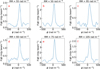 |
Fig. A.1 Faraday spectra for pixels a-f marked in Fig. 6. |
| In the text | |
Current usage metrics show cumulative count of Article Views (full-text article views including HTML views, PDF and ePub downloads, according to the available data) and Abstracts Views on Vision4Press platform.
Data correspond to usage on the plateform after 2015. The current usage metrics is available 48-96 hours after online publication and is updated daily on week days.
Initial download of the metrics may take a while.