| Issue |
A&A
Volume 708, April 2026
|
|
|---|---|---|
| Article Number | A363 | |
| Number of page(s) | 14 | |
| Section | Catalogs and data | |
| DOI | https://doi.org/10.1051/0004-6361/202558149 | |
| Published online | 23 April 2026 | |
Estimating the completeness of the QUBRICS survey with 3501 quasi-stellar object redshifts from Gaia DR3 spectra
1
INAF – Osservatorio Astronomico di Trieste,
Via G.B. Tiepolo, 11,
34143
Trieste,
Italy
2
IFPU – Institute for Fundamental Physics of the Universe,
via Beirut 2,
34151
Trieste,
Italy
3
INFN – National Institute for Nuclear Physics,
via Valerio 2,
34127
Trieste,
Italy
4
INAF – Osservatorio Astronomico di Padova,
Vicolo dell’Osservatorio 5,
35122
Padova,
Italy
5
Cerro Tololo Inter-American Observatory/NSF NOIRLab,
Casilla 603,
La Serena,
Chile
6
Dipartimento di Fisica dell’Università di Trieste, Sezione di Astronomia,
Via G.B. Tiepolo, 11,
34143
Trieste,
Italy
7
Centro de Astrofísica da Universidade do Porto,
Rua das Estrelas,
4150-762
Porto,
Portugal
8
Instituto de Astrofísica e Ciências do Espaço, Universidade do Porto,
Rua das Estrelas,
4150-762
Porto,
Portugal
9
Faculdade de Ciências, Universidade do Porto,
Rua do Campo Alegre,
4150-007
Porto,
Portugal
10
Max-Planck-Institut für Astronomie,
Königstuhl 17,
69117
Heidelberg,
Germany
11
Hamburger Sternwarte, Universität Hamburg,
Gojenbergsweg 112,
21029
Hamburg,
Germany
12
Scuola Normale Superiore Piazza dei Cavalieri,
7,
56126
Pisa,
Italy
13
SISSA – International School for Advanced Studies,
Via Bonomea 265,
34136
Trieste,
Italy
★ Corresponding author: This email address is being protected from spambots. You need JavaScript enabled to view it.
Received:
17
November
2025
Accepted:
1
March
2026
Abstract
Context. Quasi-stellar objects (QSOs) are essential for investigating the structure and evolution of the Universe. Historically, their identification has been concentrated in the northern hemisphere, primarily due to the sky coverage of major astronomical surveys. The QUBRICS (QUasars as BRIght beacons for Cosmology in the Southern hemisphere) survey, started in 2019 to address this asymmetry, has identified more than 1300 new bright (i < 19.5) high-redshift (2.5 < z < 6) QSOs in the southern sky.
Aims. This study aims to quantify, using an independent QSO sample, the completeness and recall of the QUBRICS QSO selection methods, based on extreme gradient boosting (XGB) and probabilistic random forest (PRF) techniques, since completeness is a fundamental metric for ensuring the statistical robustness of QSO-based cosmological investigations.
Methods. We analyzed a subset of Gaia DR3 sources (G < 18.25, |b| > 25 deg, negligible parallax and proper motion) with low-resolution spectra, from which we obtained a sample of 3501 QSOs. To determine how many QSOs were correctly identified as candidates, we crossmatched this independent sample with the datasets used for selection: 894 QSOs with z > 2.5 fell within the XGB dataset footprint, of which 152 were unclassified and thus eligible for completeness testing. Similarly, 675 QSOs with z > 2.5 were within the PRF dataset footprint, including 69 unclassified objects.
Results. The XGB correctly identified as candidates 136 (89%) of the 152 QSOs with z > 2.5 listed in the XGB dataset as unclassified objects. The PRF correctly identified as candidates 46 (66%) of the 69 QSOs with z > 2.5 listed in the PRF dataset as unclassified objects.
Conclusions. These findings confirm the high efficiency of the QUBRICS selection methods (recall = 89%) and provide the completeness estimate for spectroscopically confirmed QSOs (82%), which is necessary for cosmological studies that use QUBRICS data. This work also provides reliable redshifts for 1223 new QSOs (median redshift z = 2.1 and magnitude G = 17.8), which will help improve the performance of future selections.
Key words: methods: data analysis / methods: statistical / astronomical databases: miscellaneous / surveys / quasars: general
© The Authors 2026
 Open Access article, published by EDP Sciences, under the terms of the Creative Commons Attribution License (https://creativecommons.org/licenses/by/4.0), which permits unrestricted use, distribution, and reproduction in any medium, provided the original work is properly cited.
This article is published in open access under the Subscribe to Open model. This email address is being protected from spambots. You need JavaScript enabled to view it. to support open access publication.
1 Introduction
Surveys of quasi-stellar objects (QSOs) play a key role in advancing our understanding of the structure and evolution of the Universe. By studying the distribution and properties of QSOs, it is possible to gain insights into the nature of dark matter, dark energy, and other foundational aspects of physics, as well as test current theories of cosmology. Light from distant and powerful QSOs has proven to be an invaluable tool for probing the intergalactic medium (e.g., Meiksin 2009; McQuinn 2016), investigating the possible variation along cosmic time of the fundamental constants of nature (e.g., Murphy et al. 2022), and studying the development and the sources of the reionization process (e.g., Bosman et al. 2022; Dayal, Pratika et al. 2025; Madau et al. 2024); it even enables a direct measurement of the redshift drift, i.e., the temporal variation in cosmological redshifts as a probe of the Universe expansion (e.g., Liske et al. 2008). These cosmological beacons are expected to become increasingly important in the coming decade, with the upcoming availability of high-resolution spectrographs on 40m-class telescopes (e.g., ANDES/ELT; Marconi et al. 2024) that will enable the detection of the redshift drift (Trost et al. 2025, 2026). QSO surveys also enable us to probe the earliest stages of galaxy formation and the formation and evolution of supermassive black holes (e.g., Trakhtenbrot 2021), and will shed light on the processes that shape the Universe we observe today (e.g., Fan et al. 2023). Catalogs with a high completeness of confirmed bright QSOs at high redshifts are therefore essential to achieving these goals.
Surveys covering large portions of the sky (e.g., SDSS; Lyke et al. 2020) have proven very efficient in finding relatively bright QSOs at high redshifts. However, smaller-scale surveys later showed that these projects were incomplete by 30-40% (e.g., Schindler et al. 2019; Boutsia et al. 2021) at high redshifts and bright magnitudes (z ≥ 2.8, i ≤ 18), suggesting that a significant fraction of bright QSOs in the distant Universe are still undetected. Determining the completeness of QSO surveys is a critical step in achieving the aforementioned goals (e.g., computing the luminosity function) and ensuring that our understanding of the Universe is not biased.
In this paper, we test and discuss the completeness of the QUasars as BRIght beacons for Cosmology in the Southern hemisphere (QUBRICS) survey (Calderone et al. 2019). QUBRICS is a spectroscopic survey that targets bright (i < 19.5) high-redshift (z > 2,5) QSOs, with the primary goal of addressing the scarcity of bright QSOs in the southern sky caused by the historical paucity of all-sky surveys in the south. The survey utilizes photometry from the following datasets: Gaia Data Release (DR) 3 (Gaia Collaboration 2023), Panoramic Survey Telescope and Rapid Response System 1 DR2 (Pan-STARRSl; Chambers et al. 2016), SkyMapper Southern Survey (SMSS) DR4 (Onken et al. 2024), Dark Energy Survey (DES) DR2 (Abbott et al. 2021), AllWISE1 (Cutri et al. 2021), and CatWISE20201 (Marocco et al. 2021). Magnitudes for Pan-STARRS, SkyMapper, and DES are in the AB magnitude system, while Gaia, AllWISE, and CatWISE magnitudes are in the Vega system.
The QUBRICS database also integrates spectroscopic classifications and redshifts from the following primary catalogs: the Sloan Digital Sky Survey Quasar Catalog for the 16th Data Release (SDSS DR16Q) (Lyke et al. 2020), the Two-degree Field Galaxy Redshift Survey (2dFGRS, Colless et al. 2001), and the Dark Energy Spectroscopic Instrument (DESI Collaboration 2024)). These data are supplemented by additional spectroscopic classifications and redshifts from several publications (e.g., Véron-Cetty & Véron 2010; Bosman 2020; Wolf et al. 2020; Onken et al. 2022; Yang et al. 2023), as well as our own follow-up campaigns.
By using machine learning methods trained on these datasets to perform photometric candidate selection, QUBRICS observation campaigns have so far detected more than a thousand new spectroscopically confirmed bright QSOs at z > 2.5. Various methods for the selection of QSOs have been used: Calderone et al. (2019) selected candidates using canonical correlation analysis (Anderson 2003), while Guarneri et al. (2021) adopted the probabilistic random forest (PRF) algorithm (Reis et al. 2019), with modifications introduced to properly treat upper limits and missing data. Guarneri et al. (2022) further improved PRF selection, adding synthetic data to the training sets. Calderone et al. (2024) developed a method that takes advantage of the extreme gradient boosting (XGB) technique (Chen & Guestrin 2016) to significantly improve the recall of the selection algorithms (from 54% to 86%), even in the presence of severely imbalanced datasets, with the aim of extending the redshift range of the QUBRICS survey up to ~5.
In addition to the continuous improvement of the photometric selection methods, a consistent effort has been dedicated to follow-up spectroscopy (Boutsia et al. 2020; Cristiani et al. 2023). Observation runs under QUBRICS have provided reliable spectroscopic classification and redshifts for 1793 previously unidentified objects, of which 1659 (92.5%) are confirmed QSOs, with 1342 (74.8%) having a spectroscopic redshift above 2.5. The magnitude range covered is 16 < i < 19.5 and −29.5 < M 1450 < -26, while the redshift range covered is 2.5 < z < 5.8. These results confirm the effectiveness of the selection procedures and provide well-defined subsamples with statistically high completeness that allowed us to address the QSO luminosity function and cosmic reionization(s) (Boutsia et al. 2021; Grazian et al. 2022; Fontanot et al. 2023). Rare objects, such as extreme broad absorption line QSOs, discovered in the course of QUBRICS were studied by Cupani et al. (2022).
In this study we aimed to estimate the completeness and recall of the two main candidate selection methods, based on the XGB and PRF algorithms. The paper is structured as follows: Section 2 describes how the independent QSO sample was created, starting from the analysis of the Gaia DR3 spectra. Section 3 describes how the QSO sample was validated via the comparison of the redshifts of known QSOs. Section 4 describes how the QSO sample was used to measure the completeness and recall of the XGB selection. Section 5 describes how the QSO sample was used to measure the completeness and recall of the PRF selection. Section 6 discusses the reliability of the recall estimates. In Sect. 7, we analyze the obtained estimates for the completeness and discuss the results.
2 Defining an independent QSO sample to test the completeness of QUBRICS
In this study, we aimed to measure the completeness of two selection methods of QSO candidates that are central to the QUBRICS survey: the PRF-based selection, described in Guarneri et al. (2022, hereafter Paper I), and the reverseselection method, based on the XGB algorithm, described in Calderone et al. (2024, hereafter Paper II). While estimates have been produced in the context of the respective candidate selections, it is important to carry out independent assessments to ensure a reliable determination of the completeness, which is needed for the achievement of many scientific goals of QUBRICS, as well as for understanding the causes of the incompleteness.
We adopted the following definitions:
Dataset completeness: the number of true QSOs in the dataset (with or without a classification) divided by the number of true QSOs in the sky.
Spectroscopic completeness: the number of spectroscopically confirmed QSOs in the dataset divided by the number of true QSOs in the sky.
Selection recall: the number of predicted QSOs in the dataset that are actually QSOs divided by the number of true QSOs that have no classification in the dataset.
Selection completeness: the number of predicted QSOs in the dataset that are actually QSOs divided by the number of true QSOs in the sky that have no classification.
For example, consider a region of the sky with 100 QSOs in a given magnitude range. If we have a dataset where 90 of them have been detected as sources (i.e., we know their coordinates and photometric magnitudes), then the dataset completeness is 90%. If our dataset has spectroscopic classification for 30 of them, then its spectroscopic completeness is 30%. If we apply a selection algorithm on the unclassified fraction of the dataset and identify 40 of the 60 unclassified QSOs in the dataset, the recall is 66%, and the selection completeness is 60% (i.e., the recall times the dataset completeness). Thus, completeness is a measure of how comprehensive a dataset is, while recall is a measure of how good a selection algorithm is at finding all the objects of interest. If all the candidates found by the selection algorithm are observed, the resulting dataset of new objects will have a spectroscopic completeness equal to the selection completeness.
To measure these quantities, an independent QSO sample has been created, based on the Gaia DR3 main catalog (Gaia Collaboration 2023). The candidates had to have:
an associated Gaia DR3 low-resolution spectrum acquired by the onboard Blue Photometer (BP) and Red Photometer (RP);
a negligible proper motion (PM/PMerr < 3);
a negligible parallax (parallax_over_error < 3);
an apparent magnitude 14 < G < 18.252;
a galactic latitude |b| > 25 deg.
The Gaia DR3 low-resolution BP/RP spectra cover wavelength range 330-1050 nm with spectral resolution R ∼ 20-100 (Carrasco et al. 2021), sufficient to identify broad emission lines such as Lyα (1216 Å), SiIV (1397 Å) and CIV (1549 Å) at z > 2.5. The spectra of the resulting 37 504 sources have been analyzed with the method described in Sect. 3.2 of Cristiani et al. (2023): we adopted the Marz software3 (Hinton et al. 2016), which uses a cross-correlation algorithm to determine the redshift. Each spectrum is compared to a QSO template designed specifically for QSO identification and containing the emission features characteristic of QSO spectra. The algorithm computes the correlation coefficient between the spectrum and the template across the 0 < z < 5 redshift range; the redshift corresponding to the maximum correlation value is then returned as the best-fit redshift estimate. After the automatic processing with the Marz software, visual inspection was performed, in order to assign to each spectrum a subjective quality rating, QOP (Quality OPerator), and to adjust the redshift estimate when necessary (e.g., when a second cross-correlation peak provides a better agreement between the spectrum and template emission lines).
The main criteria taken into account were the maximum value of the cross-correlation between spectrum and QSO template, the signal-to-noise ratio (S/N) and the number of visible features. The resulting QOP ranged between 1 (bad: uncertain identification and/or redshift) and 4 (great: certain identification and redshift). To limit subjectivity, QOP assignments were performed following the same criteria used in Cristiani et al. (2023) and are illustrated by representative examples in Appendix B.
Considering the redshift range of interest for QUBRICS (z > 2.5) and the wavelength range of Gaia spectra (330-1050 nm), we focused on spectra that showed Lyα (1216 Å), SiIV (1397 Å) and C IV (1549 Å) emission lines clearly identifiable by visual inspection. This process resulted in 3501 Gaia spectra of sufficient quality (QOP≥ 2) to identify the corresponding objects as QSOs and measure their redshift; this corresponds to around 10% of all analyzed bright (G < 18.25) spectra. Some examples of Gaia spectra are shown in Fig. B.2: despite the low resolution, the spectra show clear emission lines that enable QSO identification. We prioritized spectral reliability by excluding uncertain objects; as a result, the sample is robust, though not fully complete. Thus, the sample does not represent the full QSO population in Gaia DR3, which is acceptable for evaluating the completeness, but should be kept in mind when interpreting the results. Since the Gaia QSO sample was selected independently from the XGB and PRF samples, we can reasonably assume that no correlation exists between the respective sources of incompleteness and that the estimate of the completeness of the XGB and PRF selection is not affected by the incompleteness in the independent sample. Therefore, we did not assess the completeness of the Gaia QSO sample itself, instead focusing exclusively on evaluating the completeness of the XGB and PRF selections relative to it.
The coordinates, magnitudes and zQU_G redshifts of these QSOs are listed in Table 1 (the full table is available at the CDS). Figure B.2 shows the Gaia spectra for the 12 QSOs with the highest redshift identified in this work. Of the 3501 QSOs, 1115 have z > 2.5 (the redshift range of interest for QUBRICS).
In Fig. 1, the distribution of the Gaia G magnitude versus the redshift determined on the basis of the Gaia low-resolution spectra is shown. The distribution appears to disfavor QSOs below z ~ 2, which is likely a selection effect due to the wavelength range of Gaia DR3 spectra: the Lyα emission line enters that specific spectral range only around z ~ 1.8.
The 12 highest-redshift QSOs discovered in this work.
 |
Fig. 1 Gaia G magnitude of the 3501 QSOs of the independent sample plotted vs. the zQU_G redshifts determined on the basis of the Gaia low-resolution spectra. The 2278 previously known QSOs are in blue, and the 1223 newly identified QSOs in red. |
3 Validating the independent QSO sample
To validate the sample of 3501 QSOs obtained from the Gaia DR3 spectra, we compared it with the objects having a spectroscopic classification in the QUBRICS database. A coordinate crossmatch has been performed, using a maximum radius of 0.5 arcseconds to avoid false matches. 2278/3501 (65%) of the objects in the sample were found to be classified as QSOs in the QUBRICS database (as of August 2024). Considering the redshift range of interest for QUBRICS (z > 2.5), 910/1115 (82%) of the objects in the sample with zQU_G > 2.5 were already classified as QSOs in the QUBRICS database. The spectroscopic completeness of the QUBRICS QSO dataset with respect to the Gaia QSO sample is thus equal to 82% for z > 2.5.
For all 2278 QSOs with a spectroscopic redshift, we compared zQu_G, the redshift measured using the Gaia spectrum, with the established spectroscopic redshift (zspec) known thanks to spectra from SDSS DR16Q (51%; Lyke et al. 2020), Véron-Cetty & Véron (2010, 19%), QUBRICS follow-up campaigns (23%), and Schindler et al. (2019, 3%), with the remaining fraction from minor sources. The comparison between the measured redshift (zQU_G) and the spectroscopic redshift (zspec) is shown in Fig. 2, where we see that there is a good agreement between the two.
The distribution of the differences ∆z = |zQU_G - zspec| was used to quantitatively estimate the compatibility between the two measures and to find any discrepancies. We applied a twostep sigma clipping procedure to identify redshift outliers. First, we computed the standard deviation of all redshift differences ∆z = |zQU_G - zspec|. Objects with ∆z > 5σ were temporarily excluded, and the standard deviation was recalculated from the remaining sample, finding σz = 0.015. This estimate of the standard deviation is robust with respect to outliers. A threshold of 5σz was chosen to identify catastrophic discrepancies: 14 objects were found to have ∆z > 5σz ≃ 0.07, all of which had a spectroscopic redshift known from the literature: 11 from the Calan-Tololo Survey (Maza et al. 1993), 2 from Véron-Cetty & Véron (2010), and 1 from SDSS DR16 (Lyke et al. 2020).
To further investigate the origin of the redshift discrepancies, we carried out follow-up spectroscopic observations for 12 of the 14 discrepant objects (all those with Dec < 0; the remaining 2 have Dec > 30 and were not visible during our observing runs). The observational details are provided in Appendix A. In all 12 cases, the newly determined spectroscopic redshifts (zSPEC_OBS) were consistent with those derived from the Gaia spectra (zQU_G; see Table A.1). These results indicate that the discrepancies were due to inaccuracies in the previously published redshifts, rather than errors in the Gaia-based measurements. The comparison with known QSOs and the spectroscopic observations demonstrate that the procedure described in Sect. 2 produces secure redshifts from Gaia low-resolution spectra, with an uncertainty of σz ~ 0.015. For this reason, we can make the following assumption: all the objects in the Gaia QSO sample are QSOs with redshift corresponding to the one measured from the low-resolution spectra (within the measured uncertainty of σz ~ 0.015).
The remaining 1223 QSOs with Gaia spectra, which did not have a known classification or spectroscopic redshift in the QUBRICS QSO dataset, have been added to the QUBRICS database. Most of these new QSOs have low redshift: the median redshift is 2.1, with 16-84 percentile range [1.84, 2.52], and only 205 have z ≥ 2.5. The median G magnitude is 17.82, with 16-84 percentile range [17.31, 18.14].
A coordinate search of the 1223 new QSOs was performed on the NASA/IPAC4 Extragalactic Database (NED)5, using a 0.5 arcsec radius (matching the value adopted for all crossmatches in this work) to ensure consistency and to minimize false associations. 168 of the 1223 new QSOs already had a published redshift in the literature, mostly from the Large Sky Area Multi-object Fiber Spectroscopic Telescope (LAMOST; Yao et al. 2019; Jin et al. 2023) and DESI (DESI Collaboration 2024) surveys, but also from photometric redshift estimates (Richards et al. 2009). The large majority of the objects, 1055, do not have a published redshift in the literature and are thus new QSO discoveries enabled by Gaia DR3 spectroscopy. These new objects will also be used to improve the training for future candidate selections.
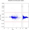 |
Fig. 2 Difference between the redshifts determined on the basis of the Gaia low-resolution spectra and the spectroscopic redshifts, ∆z, as a function of the spectroscopic redshift. The dashed red lines mark the ∆z = ±5σz threshold chosen to identify catastrophic discrepancies. |
Composition of the XGB dataset.
4 Estimating the completeness of the XGB selection
We then estimated the completeness of the QUBRICS XGB-based selection. As described in Paper II, the XGB algorithm is trained and tested on a set of spectroscopically classified objects and then is applied to a set of unclassified objects to predict their classification. The set of QSO candidates is composed by the unclassified objects predicted to be high-z QSOs by the XGB selection process.
The XGB dataset starts from the Pan-STARRS1 DR2 (Chambers et al. 2016) survey and includes all objects with:
a Pan-STARRS1DR2 magnitude yp<19;
a W1 magnitude (3.4 μm) from AllWISE or CatWISE;
a negligible proper motion (PM/PMerr < 3) from Gaia DR36;
a negligible parallax (parallax_over_error < 3) from Gaia DR36.
Unlike Paper II, we did not strictly require a matching source in Gaia DR3, so the dataset is larger by a factor of ∼2. The composition of the XGB dataset is shown in Table 2.
The last line of Table 2 presents the sources for which we could not find a spectroscopic classification, nor significant proper motion or parallax measurements in the Gaia catalog; hence, it is the subset used to search for new high-z (z > 2.5) QSO candidates. Of the 3501 QSOs of the sample defined in Sect. 2, 2713 fall within the footprint of the XGB dataset selection; of those, 894 have zQU_G ≥ 2.5.
We performed a coordinate crossmatch (radius 0.5 arcsec) between the 894 QSOs in our independent sample and the XGB dataset. We found that 18 of these QSOs were missing from the XGB dataset, corresponding to a 2% shortfall. We refer to this shortfall as “dataset incompleteness”, which we define as the fraction of QSOs that fall within the survey footprint but are absent from the dataset due to missing photometric or astrometric information. Specifically, we found that these 18 objects were not included in the XGB dataset for the following reasons:
1 lacked a Pan-STARRS1DR2 match within 0.5″;
4 had no match in AllWISE or CatWISE;
13 did not have a corresponding yp magnitude from Pan-STARRS1DR2.
The remaining 876 QSOs were successfully found in the XGB dataset, either with or without a spectroscopic classification from the QUBRICS QSO dataset. 724 have a spectroscopic classification as QSOs in the dataset, while 152 of the Gaia QSOs were unclassified and should have been selected as QSO candidates by the XGB algorithm. In fact, we find 136 of them in the XGB candidate list. The recall of the XGB candidate selection algorithm is thus 136/152 = 89%, a result in line with the estimate reported in Paper II. If we also account for the XGB dataset completeness (98%), the overall XGB selection completeness is 87%.
The 16 QSOs that were not identified as high-redshift QSO candidates were assigned the following predicted categories by the XGB:
14 low-redshift QSOs (all with 2.5 < zQU_G < 2.9);
1 star (zQU_G = 2.95);
1 galaxy (zQU_G = 3.80).
Most missed objects lie close to the z = 2.5 boundary, where photometric degeneracies with low-redshift QSOs are expected. The distribution in magnitude and redshift of the 152 unclassified QSOs is shown in Fig. 3. QSOs that have not been selected as candidates by the XGB are shown in red. The candidate selection recall remains approximately constant across magnitude and redshift, except for the lowest redshift bin: this behavior is expected, due to the lower classification accuracy for objects close to the z = 2.5 threshold on which the XGB has been trained. In fact, the large majority of the misclassified QSOs had a redshift within 0.4 from the threshold and were predicted to be low-redshift QSOs.
5 Estimating the completeness of the PRF selection
The second selection method used in the QUBRICS survey is based on the PRF algorithm (Paper I). Again, we used the independent sample defined in Sect. 2 to estimate the completeness and recall of the PRF selection.
The PRF dataset starts from the SkyMapper DR4 survey (Onken et al. 2024) and includes all objects with:
SkyMapper magnitudes 14 < i < 19;
reliable photometry (quality flag i_f la g s ≤ 4);
a W1 magnitude (3.4 μm) from CatWISE;
negligible proper motion (PM/PMerr < 3) from Gaia DR37;
negligible parallax (parallax_over_error < 3) from Gaia DR37;
a PSF-Petrosian magnitude difference smaller than 4 × a_ext8;
galactic latitude |b| > 15 deg.
Of the 3501 QSOs of the sample defined in Sect. 2, 2136 fall within the footprint of the PRF dataset selection; of those, 675 have zQU_G ≥ 2.5. We then performed a coordinate crossmatch (radius 0.5") with the PRF dataset, finding that 23 of 675 QSOs in the footprint were not included in the PRF dataset (3% dataset incompleteness), for the following reasons:
7 did not have an i magnitude from SkyMapper DR4;
7 had unreliable SkyMapper photometry ( i_flags > 4);
9 did not have a W1 magnitude from CatWISE.
The remaining 652 QSOs were successfully found in the PRF dataset, either with or without a spectroscopic classification. 69 of these had no known classification and should have been selected as QSO candidates by the PRF algorithm. Checking the candidate list, we find 46 objects out of the 69 sources: this results in a 66% recall for the PRF candidate selection method. This is slightly lower than the 67.5% estimate presented in Paper I. If we also account for the PRF dataset completeness (97%), the overall PRF selection completeness is 64%.
The 23 QSOs that were not identified as high-redshift QSO candidates were assigned the following predicted categories by the PRF:
18 low-redshift QSOs (all with 2.5 < zQU_G < 2.9);
4 stars (with 2.69 ≤ zQU_G ≤ 3.11);
1 galaxy (with zQU_G = 2.96).
The distribution in magnitude and redshift of the 69 unclassified QSOs is shown in Fig. 4. QSOs that have not been selected as candidates by the PRF are shown in red. The candidate selection recall is lower for z < 3; like the XGB case, most of the misclassified QSOs are still predicted to be low-redshift QSOs; however, unlike the XGB case, they are not concentrated in the lowest redshift bin. This is expected because the PRF is strictly a classification algorithm and does not incorporate redshift prediction, while the XGB also performs regression: this reduces the effect given by the threshold at z > 2.5 in the training set.
 |
Fig. 3 Top : histogram of the Gaia G magnitude for the 152 QSOs with no classification in the XGB sample, with the 16 QSOs that were not identified as candidates (“missed”) highlighted in red. Bottom : histogram of the zQU_G redshifts for the 152 QSOs with no classification in the XGB sample, with the 16 QSOs that were not identified as candidates (“missed”) highlighted in red. |
 |
Fig. 4 Top : histogram of the Gaia G magnitude for the 69 QSOs with no classification in the PRF sample, with the 23 QSOs that were not identified as candidates (“missed”) highlighted in red. Bottom: histogram of the zQU_G redshifts for the 69 QSOs with no classification in the PRF sample, with the 23 QSOs that were not identified as candidates (“missed”) highlighted in red. |
6 Reliability of the recall estimate
To better assess the accuracy of the recall estimates just measured, it is helpful to start from the visual representation of the datasets shown in Fig. 5. According to the definition of recall provided in Sect. 2, the recall (R) is the fraction
 (1)
(1)
where NC is the number of unclassified high-redshift QSOs in the dataset that have been selected as candidates and NU is the total number of unclassified high-redshift QSOs in the dataset.
Both NC and NU are unknown: to discover their value, all unclassified sources would need to be observed to attach a reliable classification. However, by using the Gaia QSO sample and crossmatching it with the unclassified and candidate sets (see Figs. 5 and 6), we can obtain the recall estimate (RG) as
 (2)
(2)
where NGC is the number of Gaia QSO that have been selected as candidates and NG is the total number of Gaia QSOs that are unclassified in the dataset. The recall estimates RG obtained in this way were 89% for the XGB and 66% for the PRF selection (see Sects. 4 and 5). We can derive their reliability with respect to the true recall R by making the following assumptions: (i) each of the NG unclassified Gaia QSOs is picked randomly among the unclassified QSOs, and (ii) NG ≪ NU, so the probability of picking each of the NG QSOs remains approximately constant. It follows from these assumptions that each of the NG unclassified Gaia QSOs has a probability R of being among the candidates, and a probability 1 – R of not being a candidate. Thus, the number NGC of unclassified Gaia QSOs that are also QSO candidates follows a binomial distribution, with expected value and variance:
![Mathematical equation: E[N_{GC}] = N_{G} \times R](/articles/aa/full_html/2026/04/aa58149-25/aa58149-25-eq3.png) (3)
(3)
![Mathematical equation: {\it Var}[N_{GC}] = N_{G} \times R(1-R) .](/articles/aa/full_html/2026/04/aa58149-25/aa58149-25-eq4.png) (4)
(4)
By considering the quantity RG = NGC/NG, we obtain
![Mathematical equation: E[R_G] = R](/articles/aa/full_html/2026/04/aa58149-25/aa58149-25-eq5.png) (5)
(5)
![Mathematical equation: {\it Var}[R_G] = \frac{R(1-R)}{N_{G}} .](/articles/aa/full_html/2026/04/aa58149-25/aa58149-25-eq6.png) (6)
(6)
Using the numbers NGC and NG obtained in Sects. 4 and 5, we can estimate RG, and, according to Eq. (5), this is also an estimate for R. Similarly, we can estimate an order-of-magnitude uncertainty for R by replacing R with RG in Eq. (6). For the XGB selection (Sect. 4), we have NGC = 136 and NG = 152, and hence
 (7)
(7)
For the PRF selection, we have (Sect. 5) NGC = 46 and NG = 69, and hence
 (8)
(8)
These values are valid as long as our assumptions are valid. However, since the number of unclassified QSOs NU is unknown, we should not assume a priori that NG ≪ NU and the case NG < NU should also be considered. If a significant fraction of the NU unclassified QSOs is contained in the Gaia QSO sample, then NGC deviates from a binomial distribution. Nonetheless, these values are still useful as an order-of-magnitude estimate of the uncertainty.
 |
Fig. 5 Schematic representation of the datasets used in the QUBRICS survey and in this paper. The outermost black rectangle contains all the sources within a given footprint and magnitude range. The dashed green rectangle denotes the dataset used in the XGB selection. Vertical divisions separate the sources according to their true category, while horizontal divisions separate the sources according to their label in the database. Known uninteresting sources (stars, galaxies, and low-redshift QSOs) are in the bottom-left quadrant. Known high-redshift QSOs are in the bottom-right quadrant. Unclassified sources that are stars, galaxies, or low-redshift QSOs are in the top-left quadrant. Unclassified sources that are high-redshift QSOs are in the top right. The region of interest is highlighted in cyan and by the letter U: this is the set of all true high-redshift QSOs that are unclassified in the dataset. The red rectangle represents the set of QSO candidates predicted by the XGB technique, and its intersection C with the U region is the set of unclassified high-redshift QSOs that are also candidates. The blue rectangle represents the set of Gaia QSOs, and its intersection G with the cyan U region is the set of Gaia QSOs that are unclassified in the dataset. |
 |
Fig. 6 Zoomed-in view of the region of interest (U) in Fig. 5. The intersection GC between the blue and red rectangles is the set of unclassified high-redshift QSOs in the dataset that are both QSO candidates and in the Gaia QSO sample. Completeness and recall metrics are defined in terms of these intersections in Sect. 6. |
7 Conclusions
In this work, we have presented an independent assessment of the completeness and recall of the QUBRICS QSO selection algorithms - XGB (Calderone et al. 2024) and PRF (Guarneri et al. 2022) - using a robust sample of 3501 QSOs identified from Gaia DR3 low-resolution spectra. This analysis is essential for quantifying the reliability of QUBRICS selections in view of a wide range of cosmological applications, including studies of the QSO luminosity function, cosmic reionization, and the redshift drift. We have obtained the following benchmarks:
A measure of the spectroscopic completeness (number of spectroscopically confirmed QSOs in the dataset divided by the number of true QSOs in the sky) of the QUBRICS QSO dataset with respect to the Gaia QSO sample: we find that 82% of the QSOs in the Gaia sample with z > 2.5 were already classified as QSOs in the QUBRICS dataset of spectroscopically classified sources (Sect. 3);
Estimates of the dataset completeness (number of true QSOs in the dataset divided by the number of true QSOs in the sky) for the XGB and PRF datasets: we find that 97-98% of the Gaia QSOs in dataset footprints were also present in the datasets, either as classified or unclassified objects, a reasonably high value;
Estimates of the recall (number of predicted QSOs that are actually QSOs divided by the number of true QSOs that have no classification in the dataset) for the two main selection algorithms, XGB and PRF: we find that the XGB algorithm correctly identified 89% of the unclassified Gaia QSOs in its dataset, while the PRF algorithm correctly identified 66% of the unclassified Gaia QSOs in its dataset;
Estimates of the selection completeness (number of predicted QSOs that are actually QSOs divided by the number of true QSOs in the dataset footprint without a classification): combining the dataset completeness and recall estimates, we find that the XGB-selected candidates are 87% of the unclassified Gaia QSOs in the Pan-STARRS1 footprint, while the PRF-selected candidates are 64% of the unclassified Gaia QSOs in the SkyMapper footprint.
Taken together, these results paint the overall picture of the QUBRICS survey: the completeness of spectroscopically confirmed QSOs is currently around 82%, and observing the QSO candidates provided by the XGB and PRF will increase it to ∼87% (the selection completeness).
We remark that the reliability of the recall estimates depends on the assumptions described in Sect. 6. The completeness and recall estimates derived here were computed using objects within the redshift ranges 2.5 < z < 3.4 for XGB and 2.5 < z < 3.3 for PRF (see Figs. 3 and 4). These ranges are set by the limited number of QSOs with z > 3.5 identified in the Gaia sample. Our empirical validation therefore applies mainly over the interval 2.5 < z < 3.4 (with the precise upper limit differing slightly between the XGB and PRF selections). Extrapolation beyond this redshift range should be treated with caution; however, we find no indication within our data that the selection performance changes abruptly at higher redshifts. The values for the recall are consistent with previous internal estimates (86% for XGB and 68% for PRF; Calderone et al. 2024; Guarneri et al. 2022) but now benefit from validation against an independent dataset, which strengthens their credibility.
The difference in performance between the two algorithms can be attributed to their methodological foundations. XGB, which incorporates both classification and regression, is better suited to handling imbalanced datasets and predicting redshifts, especially near the critical threshold of z ~ 2.5. In contrast, PRF is a pure classification algorithm and lacks the ability to model redshift-dependent selection effects, which likely contributes to its reduced recall. Future improvements in recall will likely require expanded training sets and the integration of additional photometric and spectroscopic surveys, such as the Vera Rubin Observatory Legacy Survey of Space and Time (Guy et al. 2025), Euclid (Euclid Collaboration: Scaramella et al. 2022; Euclid Collaboration: Mellier et al. 2025), and the Nancy Grace Roman Space Telescope (Wang et al. 2022).
Our analysis also led to the identification of 1223 new QSOs, including 205 with z > 2.5, that were previously unclassified. These objects not only enrich the QUBRICS database but also provide a valuable training set for future iterations of the selection algorithms. The validation of Gaia-derived redshifts through targeted follow-up spectroscopy confirms the reliability of the independent sample, with a redshift uncertainty (σz) of ~0.015.
From a cosmological perspective, the high recall of the XGB method ensures that QUBRICS-selected QSOs can be reliably used for statistical studies, such as measuring the QSO luminosity function and probing the intergalactic medium. The identification of candidates missed by both algorithms also highlights areas for methodological refinement, particularly in the treatment of photometric uncertainties and the inclusion of synthetic data.
In conclusion, by benchmarking the performance of the XGB and PRF algorithms against an external sample, we obtain a better understanding of their strengths and limitations. These insights will guide the refinement of future selection strategies and improve the scientific utility of QUBRICS, particularly in preparation for upcoming observational facilities such as 40m-class telescopes.
Data availability
The full version of Table 1 is available at the CDS via https://cdsarc.cds.unistra.fr/viz-bin/cat/J/A+A/708/A363.
Acknowledgements
Andrea Grazian, Stefano Cristiani, Andrea Trost, Valentina D’Odorico, Giorgio Calderone, and Matteo Porru acknowledge the financial support of the INAF GO/GTO Grant 2023 “Finding the Brightest Cosmic Beacons in the Universe with QUBRICS” (PI Grazian), and of the Italian Ministry of Education, University, and Research with PRIN 201278X4FL and the “Progetti Premiali” funding scheme. Stefano Cristiani is partly supported by the INFN PD51 INDARK grant. The work of Konstantina Boutsia is supported by NOIRLab, which is managed by the Association of Universities for Research in Astronomy (AURA) under a cooperative agreement with the U.S. National Science Foundation. Catarina Marques acknowledges the supported by FCT-Fundação para a Ciência e Tecnologia, I.P. by project reference 2023.03984.BD and DOI identifier https://doi.org/10.54499/2023.03984.BD. This work has made use of observations collected at the European Southern Observatory under ESO programme(s) 114.27HT.001. This research has made use of the SIM-BAD database, CDS, Strasbourg Astronomical Observatory, France (Wenger et al. 2000). This research has made use of the NASA/IPAC Extragalactic Database, which is funded by the National Aeronautics and Space Administration and operated by the California Institute of Technology. This work has made use of data from the European Space Agency (ESA) mission Gaia (https://www.cosmos.esa.int/gaia), processed by the Gaia Data Processing and Analysis Consortium (DPAC, https://www.cosmos.esa.int/web/gaia/dpac/consortium). Funding for the DPAC has been provided by national institutions, in particular the institutions participating in the Gaia Multilateral Agreement. This publication makes use of data products from the Wide-field Infrared Survey Explorer, which is a joint project of the University of California, Los Angeles, and the Jet Propulsion Laboratory/California Institute of Technology, funded by the National Aeronautics and Space Administration. This publication makes use of data products from the Near-Earth Object Wide-field Infrared Survey Explorer (NEOWISE), which is a joint project of the Jet Propulsion Laboratory/California Institute of Technology and the University of California, Los Angeles. NEOWISE is funded by the National Aeronautics and Space Administration. The Pan-STARRS1 Surveys (PS1) and the PS1 public science archive have been made possible through contributions by the Institute for Astronomy, the University of Hawaii, the Pan-STARRS Project Office, the Max-Planck Society and its participating institutes, the Max Planck Institute for Astronomy, Heidelberg and the Max Planck Institute for Extraterrestrial Physics, Garching, The Johns Hopkins University, Durham University, the University of Edinburgh, the Queen’s University Belfast, the Harvard-Smithsonian Center for Astrophysics, the Las Cumbres Observatory Global Telescope Network Incorporated, the National Central University of Taiwan, the Space Telescope Science Institute, the National Aeronautics and Space Administration under Grant No. NNX08AR22G issued through the Planetary Science Division of the
NASA Science Mission Directorate, the National Science Foundation Grant No. AST-1238877, the University of Maryland, Eotvos Lorand University (ELTE), the Los Alamos National Laboratory, and the Gordon and Betty Moore Foundation. The national facility capability for SkyMapper has been funded through ARC LIEF grant LE130100104 from the Australian Research Council, awarded to the University of Sydney, the Australian National University, Swinburne University of Technology, the University of Queensland, the University of Western Australia, the University of Melbourne, Curtin University of Technology, Monash University and the Australian Astronomical Observatory. SkyMapper is owned and operated by The Australian National University’s Research School of Astronomy and Astrophysics. The survey data were processed and provided by the SkyMapper Team at ANU. The SkyMapper node of the All-Sky Virtual Observatory (ASVO) is hosted at the National Computational Infrastructure (NCI). Development and support of the SkyMapper node of the ASVO has been funded in part by Astronomy Australia Limited (AAL) and the Australian Government through the Commonwealth’s Education Investment Fund (EIF) and National Collaborative Research Infrastructure Strategy (NCRIS), particularly the National eResearch Collaboration Tools and Resources (NeCTAR) and the Australian National Data Service Projects (ANDS). This project used data obtained with the Dark Energy Camera (DECam), which was constructed by the Dark Energy Survey (DES) collaboration. Funding for the DES Projects has been provided by the U.S. Department of Energy, the U.S. National Science Foundation, the Ministry of Science and Education of Spain, the Science and Technology Facilities Council of the United Kingdom, the Higher Education Funding Council for England, the National Center for Supercomputing Applications at the University of Illinois at Urbana-Champaign, the Kavli Institute of Cosmological Physics at the University of Chicago, Center for Cosmology and Astro-Particle Physics at the Ohio State University, the Mitchell Institute for Fundamental Physics and Astronomy at Texas A&M University, Financiadora de Estudos e Projetos, Fundacao Carlos Chagas Filho de Amparo, Financiadora de Estudos e Projetos, Fundacao Carlos Chagas Filho de Amparo a Pesquisa do Estado do Rio de Janeiro, Conselho Nacional de Desenvolvimento Cien-tifico e Tecnologico and the Ministerio da Ciencia, Tecnologia e Inovacao, the Deutsche Forschungsgemeinschaft and the Collaborating Institutions in the Dark Energy Survey. The Collaborating Institutions are Argonne National Laboratory, the University of California at Santa Cruz, the University of Cambridge, Centro de Investigaciones Energeticas, Medioambientales y Tecnologicas-Madrid, the University of Chicago, University College London, the DES-Brazil Consortium, the University of Edinburgh, the Eidgenossische Technische Hochschule (ETH) Zurich, Fermi National Accelerator Laboratory, the University of Illinois at Urbana-Champaign, the Institut de Ciencies de l’Espai (IEEC/CSIC), the Institut de Fisica d’Altes Energies, Lawrence Berkeley National Laboratory, the Ludwig Maximilians Universitat Munchen and the associated Excellence Cluster Universe, the University of Michigan, NSF’s NOIRLab, the University of Nottingham, the Ohio State University, the University of Pennsylvania, the University of Portsmouth, SLAC National Accelerator Laboratory, Stanford University, the University of Sussex, and Texas A&M University. This research used data obtained with the Dark Energy Spectroscopic Instrument (DESI). DESI construction and operations is managed by the Lawrence Berkeley National Laboratory. This material is based upon work supported by the U.S. Department of Energy, Office of Science, Office of High-Energy Physics, under Contract No. DE-AC02-05CH11231, and by the National Energy Research Scientific Computing Center, a DOE Office of Science User Facility under the same contract. Additional support for DESI was provided by the U.S. National Science Foundation (NSF), Division of Astronomical Sciences under Contract No. AST-0950945 to the NSF’s National Optical-Infrared Astronomy Research Laboratory; the Science and Technology Facilities Council of the United Kingdom; the Gordon and Betty Moore Foundation; the Heising-Simons Foundation; the French Alternative Energies and Atomic Energy Commission (CEA); the National Council of Humanities, Science and Technology of Mexico (CONAHCYT); the Ministry of Science and Innovation of Spain (MICINN), and by the DESI Member Institutions: www.desi.lbl.gov/collaborating-institutions. The DESI collaboration is honored to be permitted to conduct scientific research on I’oligam Du’ag (Kitt Peak), a mountain with particular significance to the Tohono O’odham Nation. Any opinions, findings, and conclusions or recommendations expressed in this material are those of the author(s) and do not necessarily reflect the views of the U.S. National Science Foundation, the U.S. Department of Energy, or any of the listed funding agencies.
References
- Abbott, T. M. C., Adamów, M., Aguena, M., et al. 2021, ApJS, 255, 20 [NASA ADS] [CrossRef] [Google Scholar]
- Anderson, T. W. 2003, An Introduction to Multivariate Statistical Analysis, 3rd edn., Wiley Series in Probability and Mathematical Statistics (Wiley) [Google Scholar]
- Banse, K., Ponz, D., Ounnas, C., Grosbol, P., & Warmels, R. 1988, in Instrumentation for Ground-Based Optical Astronomy, 431 [Google Scholar]
- Bosman, S. 2020, https://doi.org/10.5281/zenodo.15574737 [Google Scholar]
- Bosman, S. E. I., Davies, F. B., Becker, G. D., et al. 2022, MNRAS, 514, 55 [NASA ADS] [CrossRef] [Google Scholar]
- Boutsia, K., Grazian, A., Calderone, G., et al. 2020, ApJS, 250, 26 [NASA ADS] [CrossRef] [Google Scholar]
- Boutsia, K., Grazian, A., Fontanot, F., et al. 2021, ApJ, 912, 111 [NASA ADS] [CrossRef] [Google Scholar]
- Buzzoni, B., Delabre, B., Dekker, H., et al. 1984, Messenger, 38, 9 [Google Scholar]
- Calderone, G., Boutsia, K., Cristiani, S., et al. 2019, ApJ, 887, 268 [NASA ADS] [CrossRef] [Google Scholar]
- Calderone, G., Guarneri, F., Porru, M., et al. 2024, A&A, 683, A34 [NASA ADS] [CrossRef] [EDP Sciences] [Google Scholar]
- Carrasco, J. M., Weiler, M., Jordi, C., et al. 2021, A&A, 652, A86 [NASA ADS] [CrossRef] [EDP Sciences] [Google Scholar]
- Chambers, K. C., Magnier, E. A., Metcalfe, N., et al. 2016, arXiv e-prints [arXiv:1612.05560] [Google Scholar]
- Chen, T., & Guestrin, C. 2016, in Proceedings of the 22nd ACM SIGKDD International Conference on Knowledge Discovery and Data Mining, KDD ’16 (New York, NY, USA: ACM), 785 [Google Scholar]
- Clemens, J. C., Crain, J. A., & Anderson, R. 2004, in Ground-based Instrumentation for Astronomy, 5492, eds. A. F. M. Moorwood, & M. Iye, International Society for Optics and Photonics (SPIE), 331 [Google Scholar]
- Colless, M., Dalton, G., Maddox, S., et al. 2001, MNRAS, 328, 1039 [Google Scholar]
- Cristiani, S., Porru, M., Guarneri, F., et al. 2023, MNRAS, 522, 2019 [NASA ADS] [CrossRef] [Google Scholar]
- Cupani, G., Calderone, G., Selvelli, P., et al. 2022, MNRAS, 510, 2509 [NASA ADS] [CrossRef] [Google Scholar]
- Cutri, R. M., Wright, E. L., Conrow, T., et al. 2021, VizieR Online Data Catalog: AllWISE Data Release (Cutri+ 2013), VizieR On-line Data Catalog: II/328. Originally published in: IPAC/Caltech (2013) [Google Scholar]
- Dayal, Pratika, Volonteri, Marta, Greene, Jenny E., et al. 2025, A&A, 697, A211 [NASA ADS] [CrossRef] [EDP Sciences] [Google Scholar]
- DESI Collaboration (Adame, A. G., et al.) 2024, AJ, 168, 58 [NASA ADS] [CrossRef] [Google Scholar]
- >Euclid Collaboration (Scaramella, R., et al.) 2022, A&A, 662, A112 [NASA ADS] [CrossRef] [EDP Sciences] [Google Scholar]
- Euclid Collaboration (Mellier, Y., et al.) 2025, A&A, 697, A1 [Google Scholar]
- Fan, L., Fang, G., & Hu, J. 2023, Ap&SS, 368, 59 [Google Scholar]
- Fontanot, F., Cristiani, S., Grazian, A., et al. 2023, MNRAS, 520, 740 [Google Scholar]
- Gaia Collaboration (Vallenari, A., et al.) 2023, A&A, 674, A1 [NASA ADS] [CrossRef] [EDP Sciences] [Google Scholar]
- Grazian, A., Giallongo, E., Boutsia, K., et al. 2022, ApJ, 924, 62 [NASA ADS] [CrossRef] [Google Scholar]
- Guarneri, F., Calderone, G., Cristiani, S., et al. 2021, MNRAS, 506, 2471 [NASA ADS] [CrossRef] [Google Scholar]
- Guarneri, F., Calderone, G., Cristiani, S., et al. 2022, MNRAS, 517, 2436 [NASA ADS] [CrossRef] [Google Scholar]
- Guy, L. P., Bechtol, K., Bellm, E., et al. 2025, https://doi.org/10.5281/zenodo.15558559 [Google Scholar]
- Hinton, S. R., Davis, T. M., Lidman, C., Glazebrook, K., & Lewis, G. F. 2016, Astron. Comput., 15, 61 [Google Scholar]
- Jin, J.-J., Wu, X.-B., Fu, Y., et al. 2023, ApJS, 265, 25 [NASA ADS] [CrossRef] [Google Scholar]
- Liske, J., Grazian, A., Vanzella, E., et al. 2008, MNRAS, 386, 1192 [NASA ADS] [CrossRef] [Google Scholar]
- Lyke, B. W., Higley, A. N., McLane, J. N., et al. 2020, ApJS, 250, 8 [NASA ADS] [CrossRef] [Google Scholar]
- Madau, P., Giallongo, E., Grazian, A., & Haardt, F. 2024, ApJ, 971, 75 [NASA ADS] [CrossRef] [Google Scholar]
- Mainzer, A., Bauer, J., Cutri, R. M., et al. 2014, ApJ, 792, 30 [Google Scholar]
- Marconi, A., Abreu, M., Adibekyan, V., et al. 2024, SPIE Conf. Ser., 13096, 1309613 [Google Scholar]
- Marocco, F., Eisenhardt, P. R. M., Fowler, J. W., et al. 2021, ApJS, 253, 8 [Google Scholar]
- Maza, J., Ruiz, M. T., Gonzalez, L. E., Wischnjewsky, M., & Antezana, R. 1993, Rev. Mexicana Astron. Astrofis., 25, 51 [Google Scholar]
- McQuinn, M. 2016, ARA&A, 54, 313 [Google Scholar]
- Meiksin, A. A. 2009, Rev. Mod. Phys., 81, 1405 [Google Scholar]
- Murphy, M. T., Molaro, P., Leite, A. C. O., et al. 2022, A&A, 658, A123 [NASA ADS] [CrossRef] [EDP Sciences] [Google Scholar]
- Onken, C. A., Wolf, C., Bian, F., et al. 2022, MNRAS, 511, 572 [NASA ADS] [CrossRef] [Google Scholar]
- Onken, C. A., Wolf, C., Bessell, M. S., et al. 2024, PASA, 41, e061 [NASA ADS] [CrossRef] [Google Scholar]
- Reis, I., Baron, D., & Shahaf, S. 2019, AJ, 157, 16 [Google Scholar]
- Richards, G. T., Myers, A. D., Gray, A. G., et al. 2009, ApJS, 180, 67 [Google Scholar]
- Schindler, J.-T., Fan, X., McGreer, I. D., et al. 2019, ApJ, 871, 258 [NASA ADS] [CrossRef] [Google Scholar]
- Torres-Robledo, S., Briceño, C., Quint, B., & Sanmartim, D. 2020, in Astronomical Society of the Pacific Conference Series, 522, Astronomical Data Analysis Software and Systems XXVII, eds. P. Ballester, J. Ibsen, M. Solar, & K. Shortridge, 533 [Google Scholar]
- Trakhtenbrot, B. 2021, in Nuclear Activity in Galaxies Across Cosmic Time, 356, eds. M. Povic, P. Marziani, J. Masegosa, H. Netzer, S. H. Negu, & S. B. Tessema, 261 [Google Scholar]
- Trost, A., Marques, C. M. J., Cristiani, S., et al. 2025, A&A, 699, A159 [NASA ADS] [CrossRef] [EDP Sciences] [Google Scholar]
- Trost, A., Marques, C. M. J., Cristiani, S., et al. 2026, arXiv e-prints [arXiv:2603.02318] [Google Scholar]
- Véron-Cetty, M. P., & Véron, P. 2010, A&A, 518, A10 [Google Scholar]
- Wang, Y., Zhai, Z., Alavi, A., et al. 2022, ApJ, 928, 1 [Google Scholar]
- Wenger, M., Ochsenbein, F., Egret, D., et al. 2000, A&AS, 143, 9 [NASA ADS] [Google Scholar]
- Wolf, C., Hon, W. J., Bian, F., et al. 2020, MNRAS, 491, 1970 [NASA ADS] [CrossRef] [Google Scholar]
- Wright, E. L., Eisenhardt, P. R. M., Mainzer, A. K., et al. 2010, AJ, 140, 1868 [Google Scholar]
- Yang, J., Fan, X., Gupta, A., et al. 2023, ApJS, 269, 27 [NASA ADS] [CrossRef] [Google Scholar]
- Yao, S., Wu, X.-B., Ai, Y. L., et al. 2019, ApJS, 240, 6 [NASA ADS] [CrossRef] [Google Scholar]
The AllWISE and CatWISE catalogs combine data from the Widefield Infrared Survey Explorer Wright et al. (2010) and Near-Earth Object Wide-Field Infrared Survey Explorer Mainzer et al. (2014) missions.
2 The magnitude range 14 < G < 18.25 was chosen pragmatically to keep the visually inspected sample manageable (resource-driven choice), while still focusing on the brightest sources with an acceptable S/N.
The National Aeronautics and Space Administration (NASA) and the Infrared Processing and Analysis Center (IPAC) fund and maintain the NED archive.
Sources with PM/PMerr > 3 or parallax_over_error > 3 from Gaia DR3 were excluded from the dataset, while sources with PM/PMerr ≤ 3 and parallax_over_error ≤ 3, or with no matching source in Gaia DR3 were included.
Sources with PM/PMerr > 3 or parallax_over_error > 3 from Gaia DR3 were excluded from the dataset, while sources with PM/PMerr ≤ 3 and parallax_over_error ≤ 3, or with no matching source in Gaia DR3 were included.
σ_ext is calculated as the average of the normalized PSF-Petrosian magnitude differences in i and z bands, where each band's difference is normalized by measurement errors and calibrated relative to the median difference for objects of similar magnitude.
Appendix A Spectroscopic observations of discrepant redshifts
Twelve QSOs with redshift discrepancies between the literature and the present Gaia estimate (Table A.1) have been observed with follow-up spectroscopy at the Southern Astrophysical Research (SOAR) and European Southern Observatory (ESO) New Technology Telescope (NTT) telescopes using the Goodman High-Throughput Spectrograph (GHTS; Clemens et al. 2004) and ESO Faint Object Spectrograph 2 (EFOSC2; Buzzoni et al. 1984) instruments, respectively. Figure A.1 shows the spectra obtained from the observations.
Seven candidates were observed in September and October 2024 at the SOAR telescope, using the Goodman High Throughput Spectrograph with the Red camera and the 4001/mm Volume Phase Holographic (VPH) grating (wavelength range λ ~ 5000 – 9000 Å and resolution ∼ 1850), with exposure times between 600 and 900 s. 4 more candidates were observed with Goodman in May 2025, using the Blue camera and the 400l/mm VPH grating (wavelength range λ ∼ 3000 – 7050 Å and resolution ∼ 1850). All Goodman data were obtained during engineering time. One candidate was observed in November 2024, as a part of an observing program at the ESO NTT (PI. A. Grazian, proposal 114.27HT.001), employing the EFOSC2 instrument and Grism #13 (wavelength range λ ∼ 3700 – 9300 Å and resolution ∼ 1000), with exposure time of 600 s.
Data obtained with EFOSC2 were reduced with a custom pipeline based on MIDAS scripts (Banse et al. 1988). Each spectrum has been processed to subtract the bias and normalized by the flat; wavelength calibration is achieved using helium, neon and argon lamps, finding a rms of ∼ 0.5Å; flux calibration was performed using spectroscopic flux standards observed at the beginning of the night. Data obtained with GHTS were reduced using the custom Goodman reduction pipeline (Torres-Robledo et al. 2020) that applies bias subtraction, flat field correction and wavelength calibration to each individual science frame. Flux calibration was performed using spectroscopic flux standards observed at the beginning of the night. Observing conditions have not always been photometric.
All 12 QSOs turned out to have a spectroscopic redshift in excellent agreement with the redshift from the Gaia low-resolution spectra (Table A.1). This further confirms the validity of the redshift measurements of the independent sample.
Appendix B Examples of Gaia DR3 spectra
Figure B.1 contains examples of 12 Gaia DR3 spectra showing the four QOP quality levels used in this work (see Sect. 2). QOP=1 (top): uncertain identification with low-S/N and ambiguous features; QOP=2 (second): acceptable quality with identifiable but weak emission lines; QOP=3 (third): good quality with clear emission lines enabling secure classification; QOP=4 (bottom): excellent quality with strong emission lines and high S/Ns. Only QOP≥2 objects were included in our analysis to ensure reliable redshift measurements. A further proof of the quality of Gaia spectra is shown in Fig. B.2, which contains the Gaia DR3 spectra of the 12 QSOs with the highest redshift among the new identifications obtained in this work (corresponding to the objects listed in Table 1).
Spectroscopic observations of 12 QSOs with discrepant redshifts.
 |
Fig. A.1 Gaia spectra (in blue) and Goodman/EFOSC2 spectra (in red) for the 12 observed objects with redshift discrepancies between the literature and the present Gaia estimate (see Table A.1). Observations confirm in all cases the Gaia estimates. |
 |
Fig. B.1 Gaia DR3 spectra of different qualities: QOP=1 (first row), QOP=2 (second), QOP=3 (third), and QOP=4 (fourth). |
All Tables
All Figures
|
Fig. 1 Gaia G magnitude of the 3501 QSOs of the independent sample plotted vs. the zQU_G redshifts determined on the basis of the Gaia low-resolution spectra. The 2278 previously known QSOs are in blue, and the 1223 newly identified QSOs in red. |
| In the text | |
|
Fig. 2 Difference between the redshifts determined on the basis of the Gaia low-resolution spectra and the spectroscopic redshifts, ∆z, as a function of the spectroscopic redshift. The dashed red lines mark the ∆z = ±5σz threshold chosen to identify catastrophic discrepancies. |
| In the text | |
|
Fig. 3 Top : histogram of the Gaia G magnitude for the 152 QSOs with no classification in the XGB sample, with the 16 QSOs that were not identified as candidates (“missed”) highlighted in red. Bottom : histogram of the zQU_G redshifts for the 152 QSOs with no classification in the XGB sample, with the 16 QSOs that were not identified as candidates (“missed”) highlighted in red. |
| In the text | |
|
Fig. 4 Top : histogram of the Gaia G magnitude for the 69 QSOs with no classification in the PRF sample, with the 23 QSOs that were not identified as candidates (“missed”) highlighted in red. Bottom: histogram of the zQU_G redshifts for the 69 QSOs with no classification in the PRF sample, with the 23 QSOs that were not identified as candidates (“missed”) highlighted in red. |
| In the text | |
|
Fig. 5 Schematic representation of the datasets used in the QUBRICS survey and in this paper. The outermost black rectangle contains all the sources within a given footprint and magnitude range. The dashed green rectangle denotes the dataset used in the XGB selection. Vertical divisions separate the sources according to their true category, while horizontal divisions separate the sources according to their label in the database. Known uninteresting sources (stars, galaxies, and low-redshift QSOs) are in the bottom-left quadrant. Known high-redshift QSOs are in the bottom-right quadrant. Unclassified sources that are stars, galaxies, or low-redshift QSOs are in the top-left quadrant. Unclassified sources that are high-redshift QSOs are in the top right. The region of interest is highlighted in cyan and by the letter U: this is the set of all true high-redshift QSOs that are unclassified in the dataset. The red rectangle represents the set of QSO candidates predicted by the XGB technique, and its intersection C with the U region is the set of unclassified high-redshift QSOs that are also candidates. The blue rectangle represents the set of Gaia QSOs, and its intersection G with the cyan U region is the set of Gaia QSOs that are unclassified in the dataset. |
| In the text | |
|
Fig. 6 Zoomed-in view of the region of interest (U) in Fig. 5. The intersection GC between the blue and red rectangles is the set of unclassified high-redshift QSOs in the dataset that are both QSO candidates and in the Gaia QSO sample. Completeness and recall metrics are defined in terms of these intersections in Sect. 6. |
| In the text | |
|
Fig. A.1 Gaia spectra (in blue) and Goodman/EFOSC2 spectra (in red) for the 12 observed objects with redshift discrepancies between the literature and the present Gaia estimate (see Table A.1). Observations confirm in all cases the Gaia estimates. |
| In the text | |
|
Fig. B.1 Gaia DR3 spectra of different qualities: QOP=1 (first row), QOP=2 (second), QOP=3 (third), and QOP=4 (fourth). |
| In the text | |
 |
Fig. B.2 Gaia spectra of the 12 highest-redshift QSOs discovered in this work (see Table 1). |
| In the text | |
Current usage metrics show cumulative count of Article Views (full-text article views including HTML views, PDF and ePub downloads, according to the available data) and Abstracts Views on Vision4Press platform.
Data correspond to usage on the plateform after 2015. The current usage metrics is available 48-96 hours after online publication and is updated daily on week days.
Initial download of the metrics may take a while.