| Issue |
A&A
Volume 708, April 2026
|
|
|---|---|---|
| Article Number | A360 | |
| Number of page(s) | 13 | |
| Section | Extragalactic astronomy | |
| DOI | https://doi.org/10.1051/0004-6361/202557921 | |
| Published online | 27 April 2026 | |
Stellar halos of bright central galaxies
II. Scaling relations, colors and metallicity evolution with redshift
1
Department of Astronomy and Yonsei University Observatory, Yonsei University, 50 Yonsei-ro, Seodaemun-gu, Seoul 03722, Republic of Korea
2
INAF Osservatorio Astronomico di Capodimonte, Salita Moiariello 16, 80131 Napoli, Italy
★ Corresponding authors: This email address is being protected from spambots. You need JavaScript enabled to view it.
; This email address is being protected from spambots. You need JavaScript enabled to view it.
Received:
31
October
2025
Accepted:
6
March
2026
Abstract
Aims. We investigate the formation and evolution of stellar halos (SHs) around bright central galaxies (BCGs), focusing on their scaling relations, colors, and metallicities across cosmic time, and we compare model predictions with ultra-deep imaging data.
Methods. We used the semianalytic model FEGA25, applied to merger trees from high-resolution dark matter simulations, including an updated treatment of intracluster light (ICL) formation. SHs are defined as the stellar component within a physically motivated transition radius, linked to the structural properties of the host halo. Predictions are compared with observations from the VST Early-type GAlaxy Survey (VEGAS) and Fornax Deep Survey (FDS).
Results. The SH mass correlates well with the BCG and ICL masses, with tighter scatter in the SH–ICL relation. The transition radius peaks at 30−40 kpc nearly independent of redshift in the model predictions, but can reach ∼400 kpc in the most massive halos, after z = 0.5. SHs and ICL show nearly identical color distributions at all epochs, both reddening toward z = 0. At z = 2, SHs and the ICL are ∼0.4 dex more metal–poor than BCGs, but the gap shrinks to ∼0.1 dex by the present time. Observed colors are consistent with model predictions, while observed metallicities are lower, suggesting a larger contribution from disrupted dwarfs.
Conclusions. SHs emerge as transition regions between BCGs and the ICL, dynamically and chemically coupled to both. Their properties depend on halo concentration, ICL formation efficiency, and the progenitor mass spectrum. Upcoming wide–field photometric and spectroscopic surveys (e.g. LSST, WEAVE, 4MOST) will provide crucial tests by mapping structure, metallicity, and kinematics in large galaxy samples.
Key words: galaxies: evolution / galaxies: formation
© The Authors 2026
 Open Access article, published by EDP Sciences, under the terms of the Creative Commons Attribution License (https://creativecommons.org/licenses/by/4.0), which permits unrestricted use, distribution, and reproduction in any medium, provided the original work is properly cited.
This article is published in open access under the Subscribe to Open model. This email address is being protected from spambots. You need JavaScript enabled to view it. to support open access publication.
1. Introduction
Stellar halos (SHs) are diffuse, low surface brightness (LSB) stellar envelopes that surround galaxies and preserve a fossil record of past accretion events and early phases of in situ star formation (Bullock & Johnston 2005; Cooper et al. 2010). Their study has become a cornerstone for understanding the hierarchical buildup of galaxies within the Λ Cold Dark Matter (ΛCDM) framework, since halo stars are long-lived and retain chemical and dynamical imprints of their progenitors (Helmi 2008; Font et al. 2011; Duc et al. 2015; Iodice et al. 2016; Lane et al. 2022; Beltrand et al. 2024).
Photometric surveys of resolved red giant branch (RGB) stars in nearby galaxies have shown that colors can serve as robust proxies for metallicity under reasonable assumptions about stellar ages (Monachesi et al. 2016; Harmsen et al. 2017). These surveys revealed a remarkable diversity: while some halos display strong negative color and metallicity gradients (bluer, more metal-poor populations at larger radii), others show almost flat profiles over tens of kiloparsecs (Mouhcine et al. 2005; Ibata et al. 2014). In the Milky Way, spectroscopic surveys have established a clear dichotomy between the inner halo, which is relatively rich in metals, and the outer halo, which is poorer in metals. This is consistent with a two-component formation scenario (Carollo et al. 2007; Beers et al. 2012; Deason et al. 2014; Helmi et al. 2018). Similarly, M31 exhibits a pronounced metallicity gradient that extends to large radii, suggesting that its halo has been significantly shaped by the accretion of relatively massive satellites (Kalirai et al. 2006; Gilbert et al. 2014).
A key emerging result is that SH metallicities correlate with the host galaxy stellar mass or luminosity: more massive galaxies tend to host more metal-rich halos. This relation is consistent with expectations from the mass–metallicity relation of dwarf satellites (Mouhcine et al. 2005; Harmsen et al. 2017; D’Souza & Bell 2018). However, the halo-to-halo scatter is large, which reflects the stochasticity of hierarchical assembly and the diversity of accretion histories (Merritt et al. 2016; Amorisco 2017). Chemical abundance ratios, particularly [α/Fe], provide further constraints: high [α/Fe] ratios trace rapid star formation in massive progenitors or in situ components, while lower values indicate extended star formation in low-mass dwarfs (Venn et al. 2004; Deason et al. 2016).
Recently, ultradeep wide-field photometric surveys have extended SH studies to a wider variety of environments, including galaxy groups and clusters. The Very large Survey Telescope (VST) Early-type GAlaxy Survey (VEGAS) survey has revealed extended halos, tidal features, and intracluster light (ICL) in several nearby systems (Capaccioli et al. 2015; Iodice et al. 2017, 2019; Spavone et al. 2017, 2018, 2020, 2021, 2022, 2024; Ragusa et al. 2023). The studies just quoted highlight the strong connection between the outer envelopes of massive early-type galaxies (ETGs) and their accretion histories, with signatures of past mergers, stripping, and disruption events. These results complement stellar population studies in the Local Group and extend SH science to a statistical sample of galaxies in diverse environments.
Theoretical models and cosmological simulations have been instrumental in interpreting these observations. Early semianalytic and particle-tagging models highlighted the role of a few dominant progenitors in building up halos (Bullock & Johnston 2005; Cooper et al. 2010). More recent hydrodynamical simulations, such as AURIGA (Grand et al. 2017), FIRE (Hopkins et al. 2014), and IllustrisTNG (Nelson et al. 2018), demonstrated that accreted and in situ components are important: in situ stars are typically richer in metals and centrally concentrated, which produces steeper gradients, whereas accreted halos are flatter unless they were shaped by the disruption of massive satellites (Font et al. 2011; Pillepich et al. 2018; Monachesi et al. 2019; Elias et al. 2020). In summary, studies of SH colors and metallicities revealed a complex and diverse picture. Observations indicate correlations with host mass and stochastic variations tied to the accretion history, while simulations stress the interplay between in situ star formation and accreted material (e.g., Cooper et al. 2015; Wright et al. 2024). Future wide-field imaging surveys and spectroscopic campaigns such as the LSST (Ivezić et al. 2019), WEAVE (Jin et al. 2024), and 4MOST (de Jong et al. 2019) will expand the halo samples to statistically significant sizes, enabling robust comparisons with cosmological models and yielding new insights into galaxy formation and evolution (Cooper et al. 2011; Helmi 2020; Spavone et al. 2022).
Recent simulation suites have substantially expanded the statistics and physical realism for SH studies. The augmented AURIGA project adds 40 new Milky Way-mass zooms (plus 26 dwarf-mass systems) at fixed physics, enabling stronger constraints on the halo-to-halo scatter in ex situ fractions, metallicity gradients, and their connection to merger histories (Grand et al. 2017). Within AURIGA, new analyses connect the strongly radially anisotropic debris and steep negative [Fe/H] gradients to the dominance of one or a few massive accretion events, refining and extending earlier gradient-assembly correlations (e.g., Gaia–Sausage–Enceladus-like progenitors; Belokurov et al. 2018; Helmi et al. 2018).
In the cluster regime, the TNG-Cluster project (Nelson et al. 2024) opens the door to statistical studies of BCGs+SHs+ICL within the same galaxy-formation model as IllustrisTNG. First results map stellar and intracluster medium (ICM) properties and assembly histories, providing a framework for tracing ex situ buildup and outer-envelope growth at high masses. Complementary large-volume and comparison projects strengthen these trends. In The Three Hundred hydrodynamical simulations (Cui et al. 2018), the ICL fraction correlates with the cluster dynamical state, supporting a picture in which late-time accretion and tidal processing grow diffuse outer components. This inference is directly relevant to massive-galaxy SHs and their metallicity gradients in dense environments (Contreras-Santos et al. 2024). At group/cluster scales in TNG300 (Nelson et al. 2019), recent work revisited BCG growth and the timing of ex situ assembly, highlighting late-time outer-envelope buildup and providing predictions for metallicity and age trends with radius that can be compared with deep imaging and spectroscopy (Montenegro-Taborda et al. 2023).
Finally, related zoom studies continue to clarify the in situ versus accreted imprint on chemo-kinematics. Edge-on maps in AURIGA connecting age–metallicity–[α/Fe] to merger-driven heating offer templates for interpreting thick-disk/inner-halo overlaps and their projected gradients. These maps emphasize that spherically averaged metallicity profiles are intrinsically steeper than minor-axis projections, which are typically measured observationally (Pinna et al. 2024).
We expand upon the analysis presented by Contini et al. (2024d), where we first implemented SH formation in our semianalytic model of galaxy formation. Here, we investigate the main scaling relations between SH and BCG–ICL mass and between SH mass and the transition radius in the first part, followed by an analysis of their colors and metallicities as a function of redshift from z = 2 down to the present time in the second part.
The remainder of the paper is structured as follows. In Section 2 we describe the implementation of SH formation in our model and provide details about the simulations and the accompanying observational data. In Section 3 we present our analysis and highlight and discuss the main results. Finally, in Section 4, we summarize the key conclusions. Unless otherwise stated, stellar and halo masses are corrected for h = 0.68, and stellar masses are derived assuming a Chabrier initial mass function (Chabrier 2003).
2. Methods
For the analysis that follows in Section 3, we took advantage of the FEGA25 (Formation and Evolution of GAlaxies) dedicated semianalytic model, in its latest version as detailed in Contini et al. (2025b), specifically, with the AGNeject1 option for the hot-gas ejection mode driven by active galactic nuclei (AGNs) feedback (see Contini et al. 2025a for further details). FEGA25 implements updated prescriptions for baryonic physics, including positive AGN feedback, a renewed supernova (SN) feedback scheme, and a more sophisticated star formation law (Contini et al. 2024d).
2.1. Semianalytic model and ICL formation
Since the key focus of this work is the redshift evolution of the main properties of SHs, we begin with a detailed description of their formation. Because SHs originate from the diffuse light, or ICL, we first provide a brief summary of its formation. In FEGA25, the ICL arises through several channels, whose relative importance varies throughout its assembly history. The three main channels are stellar stripping, mergers, and preprocessing. Stellar stripping of satellite galaxies contributes a significant fraction of diffuse light, as stars are removed from satellites due to the potential well of the host halo. In some rare cases, tidal forces can be strong enough to completely disrupt a satellite galaxy.
Another important channel is represented by mergers of central and satellite galaxies (both minor and major mergers). At each merger event, the code assigns a fraction of the satellite stars to the ICL component associated with the central galaxy, with an average of 20% and a scatter of ±5%. The last channel is preprocessing, which can be considered a subchannel, since preprocessed ICL ultimately originates from either stellar stripping or mergers (or both). In short, preprocessed diffuse light forms in halos other than that of the central galaxy and is subsequently accreted when these halos merge with the host.
In Contini et al. (2024a), and previously also in Contini et al. (2023), we showed that stellar stripping is the dominant channel of ICL formation, while mergers play a secondary role. However, as repeatedly discussed in earlier works, the net balance between the two channels strongly depends on the definition of mergers (see, e.g., Contini et al. 2018 for a detailed discussion, as well as Joo et al. 2025; Gendron & Martel 2025 for comparisons). We stress here that in the model, the ICL is a physically motivated component whose mass and spatial distribution are determined by the cumulative effects of these processes in the halo assembly history, and are not imposed by construction.
2.2. Definition of the stellar halo and transition radius
In FEGA25, the SH forms directly from stars originally belonging to the ICL. The first implementation was introduced in Contini et al. (2024b) through the definition of a transition region between the central galaxy (CG) and the ICL, itself defined as the stars within the transition radius Rtrans. This radius is linked to the halo concentration, which is computed on the basis of a Navarro-Frenk-White (NFW) dark matter distribution (Navarro et al. 1997). The ICL concentration is directly tied to the halo concentration via the following equation:
 (1)
(1)
where R200 and Rs, DM represent the virial and scale radii of the DM halo, respectively, Rs, ICL is the scale radius of the ICL mass distribution, and γ is a parameter quantifying how much more concentrated the ICL is than the DM. This parameter was calibrated in Contini et al. (2024b) using a Markov chain Monte Carlo algorithm, and it typically ranges between 1 and 3. This model assumes that the ICL distribution follows an NFW profile (see, e.g., Contini & Gu 2020 for further details), but with a higher concentration. From Equation (1), the transition radius Rtrans is then defined as
 (2)
(2)
which essentially is the analog of the NFW scale radius for the ICL.
To model the SH, we assumed that all stars belonging to the ICL and lying within the transition radius form the SH, which is considered as an intermediate region between the CG and the ICL. It must be noted that this implementation does not explicitly determine whether these stars are gravitationally bound to the central galaxy. Consequently, the SH can be regarded either as a distinct third component of the BCG+SH+ICL system or as a transition zone. Stars can move between the ICL and SH components, and in certain conditions, they can migrate from the SH to the BCG. By construction, the SH mass is therefore closely linked to the ICL mass and spatial distribution. In particular, a correlation between SH and ICL mass is an expected outcome of the adopted definition, while the residual scatter reflects variations in halo concentration, ICL formation efficiency, and the detailed assembly history of the system.
Two additional criteria regulate this process. First, when the transition radius Rtrans lies within the bulge radius, all SH stars within it are transferred to the bulge. Second, for stability reasons, the SH mass cannot exceed the stellar mass of the BCG (bulge+disk)1. Any excess mass in the SH is redistributed to the BCG disk. These stability criteria imply that the SH mass is not a fixed fraction of the ICL mass, even at fixed halo mass or concentration, and they introduce physically motivated scatter in all SH-related scaling relations.
As highlighted above, the SH stars may or may not be bound to the central galaxy. In the first case, the SH can be interpreted as a third component of the BCG+SH+ICL system, while in the second case or in the mixed case with bound and unbound stars, it represents a transition region between the galaxy and the surrounding ICL. Following Contini et al. (2024b), who first implemented SHs, we adopted the latter interpretation. Thus, the system was modeled as a central galaxy, consisting of a bulge and disk, surrounded by an SH, all embedded in a more extended diffuse-light component (see Figure 1 for a schematic illustration). We therefore emphasize that the interpretation of SHs as transition regions is a direct consequence of the adopted definition, while the quantitative trends in their mass, structure, and stellar populations explored in Section 3 reflect genuine physical dependences on halo concentration, ICL assembly, and satellite accretion.
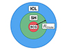 |
Fig. 1. Schematic representation of central galaxies and their surrounding stellar halos and intracluster stars. The stellar halo is defined as the stellar component within the transition radius Rtrans, marking the intermediate region between the galaxy and the intracluster light. |
Although the definition of the transition radius is somewhat arbitrary, we showed in Contini et al. (2024b) that the typical values of Rtrans for halos of a given mass are consistent with observations and theoretical predictions, such as the relation found by Proctor et al. (2024). It is also worth discussing an important caveat. The observational definition of the SH is not unique. Historically, the integrated-light profiles of the Milky Way and other disk galaxies were successfully fit by a de Vaucouleurs component dominating the central regions and the outskirts, which led to the interpretation of the SH as a photometric extension of the bulge (e.g., de Vaucouleurs 1959). A purely morphological classification does not capture the physical distinctiveness of the halo, whose stars typically exhibit low metallicities, dispersion-dominated kinematics, and signatures of accretion and minor merging (e.g., Carollo et al. 2007, 2010; Helmi 2008; Deason et al. 2013; Belokurov et al. 2020). This is particularly clear in the Milky Way, where Gaia has revealed that a significant fraction of the inner halo originates from a major accretion event (Gaia-Enceladus; Helmi et al. 2018; Belokurov et al. 2018), and where chemical and kinematic surveys identified multiple substructures and a dual-halo configuration. We therefore adopted a physical definition of the SH based on dynamical selection criteria and not on a decomposition of the light profile alone. This approach reflects modern observational evidence that the halo traces the hierarchical assembly history of the host galaxy and is distinct from bulge and disk components in origin and in stellar population properties (e.g., Gallart et al. 2019; Naidu et al. 2020).
2.3. Stellar populations: Colors and metallicities
The model tracks the age and metallicity of the stellar populations associated with each stellar component (BCG, SH, and ICL) by following their star formation and chemical enrichment histories self-consistently within the semianalytic framework. Broadband colors are computed by applying stellar population synthesis models to the predicted stellar mass, age, and metallicity of each component, assuming a Chabrier initial mass function.
In this approach, colors and metallicities are not free parameters tuned to reproduce the observations, but are direct outputs of the model, inherited from the formation histories of the different stellar components. In particular, the SH and the ICL are assumed to evolve passively after their formation, without in situ star formation, which is consistent with their predominantly accreted origin.
Mean metallicities are derived using the same mass-weighting scheme as adopted for the computation of colors to ensure a coherent mapping between the semianalytic outputs and the observable quantities used in the comparison with data. While stellar populations represent one of the most challenging aspects to model within a semianalytic framework, this method allows us to perform a physically motivated and internally consistent comparison between model predictions and observations. In the remainder of this section, we briefly describe the merger trees (Section 2.4) and the observational dataset (Section 2.5) before we move on to the analysis and discussion of the main results.
2.4. Merger trees
In order to construct galaxy catalogs, semianalytic models require merger trees extracted from dark matter-only numerical simulations. For this purpose, we employed a set of three cosmological simulations carried out with the latest version of the GADGET code, namely GADGET-4 (Springel et al. 2021). These simulations span different volumes and mass resolutions, as summarized in Table 1, and the corresponding merger trees were used to generate the inputs for FEGA25.
Parameters of the simulations and thresholds chosen.
All runs adopted the same comoving gravitational softening length of 3 kpc/h2 and followed the Planck 2018 cosmology (Planck Collaboration VI 2020): Ωm = 0.31 for the matter density parameter, ΩΛ = 0.69 for the cosmological constant, ns = 0.97 for the primordial spectral index, σ8 = 0.81 for the power spectrum normalization, and h = 0.68 for the dimensionless Hubble parameter. The simulations were evolved from an initial redshift of z = 63 to the present day, with data stored in 100 snapshots uniformly distributed in cosmic time between z = 20 and z = 0.
We note that the numerical resolution can play an important role when the same halos are simulated at different resolutions, particularly for quantities related to satellite survival, stripping, and mass loss (e.g. Contini et al. 2014). However, this effect has been explicitly tested in previous work, where we verified that in the halo-mass ranges where different simulations overlap, the predicted properties of diffuse stellar components are consistent within the intrinsic scatter. Nevertheless, in Appendix A, we provide some additional plots that separate the data from the different runs.
Because of the different resolutions of the simulations, we imposed distinct mass thresholds when selecting dark matter main halos (focusing exclusively on centrals), as listed in Table 1. The largest-volume run, YS300, provided a statistically significant sample of massive groups and clusters, while the highest-resolution box enabled us to probe Milky Way-sized halos. This combined catalog forms the basis for the analysis presented in Section 3.
2.5. Observed data
To compare the predictions of our model with observational data, we used the survey VEGAS (Capaccioli et al. 2015; Iodice et al. 2021) and the Fornax Deep Survey (FDS; Iodice et al. 2016). These surveys do not provide metallicity measurements. For the same targets, we therefore complemented them with data from the Fornax3D project (F3D; Sarzi et al. 2018) and the M3G survey (Krajnović et al. 2018). Throughout the rest of the paper, we refer to this combined dataset simply as VEGAS, which includes colors and metallicity information.
VEGAS is a wide-field deep imaging program conducted with the VLT Survey Telescope (VST) at ESO’s Paranal Observatory. Its primary aim is to explore the faint outskirts of nearby ETGs down to very low surface brightness levels, typically reaching μg ∼ 28.5 − 29 mag arcsec−2 (Iodice et al. 2021). By combining multiband wide-field and deep optical imaging (u, g, r, i), VEGAS allows for a detailed study of the structural properties and stellar populations in the outer regions of galaxies, unveiling faint SHs, extended envelopes, and substructures such as shells, streams, and tidal debris, which are relics of past accretion and merging events (Mihos et al. 2017).
In addition, VEGAS plays a crucial role in the investigation of the ICL. This component provides direct constraints on the assembly history of massive structures and the efficiency of tidal stripping and galaxy interactions (Contini et al. 2014; Montes & Trujillo 2018; Spavone et al. 2020). By building a statistical sample of ETGs across diverse environments, from isolated systems to dense clusters, VEGAS delivers a key observational benchmark for hierarchical galaxy formation models and for the study of the stellar mass assembly at large radii (Cooper et al. 2010; Pillepich et al. 2018). For further details and references about the survey, we refer to Contini et al. (2024b).
The Fornax Deep Survey (FDS) is a deep optical imaging program carried out with the VST as part of the VEGAS collaboration. Its main goal is to map the entire Fornax cluster to unprecedented surface-brightness levels of about μg ∼ 29 mag arcsec−2, and thus, to provide the first homogeneous and contiguous photometric coverage of the cluster core and its periphery (Iodice et al. 2016). With a wide field of view of one square degree per pointing and multiband coverage (u, g, r, i), FDS enables a systematic exploration of the galaxy population of Fornax, ranging from early- and late-type systems to ultradiffuse galaxies and low surface brightness dwarfs (Venhola et al. 2017, 2018).
A key strength of FDS is its ability to trace the ICL and the extended stellar envelopes of massive galaxies, which represent direct evidence of the ongoing cluster assembly and provide insights into tidal stripping, galaxy harassment, and merging processes (Iodice et al. 2017; Spavone et al. 2017). Moreover, by resolving faint structural and color gradients across galaxies, the survey constrains the stellar populations and metallicity distributions, thereby shedding light on environmental transformation processes and their role in shaping galaxy evolution within dense environments.
The FDS is one of the deepest wide-area optical surveys of a nearby cluster, complementing similar campaigns in Virgo and Coma. By simultaneously resolving the brightest galaxies and the faintest dwarf systems, it delivers a comprehensive view of galaxy evolution in clusters and offers crucial observational constraints for cosmological models of structure formation (Drinkwater et al. 2001; Capaccioli et al. 2015). For further details about the FDS, we refer to Iodice et al. (2016).
We note that while VEGAS primarily targets bright central galaxies, the FDS sample includes a significant fraction of satellite systems. For this reason, FDS data were not used here as a direct counterpart of the simulated sample, which only includes central galaxies. Instead, FDS provides a complementary reference for the properties of diffuse outer stellar components in a dense cluster environment. The comparison with model predictions is therefore statistical in nature and is not intended as a one-to-one correspondence between individual observed and simulated systems. This comparison therefore provides a consistency check on the typical scales and trends of diffuse stellar components and is no direct test of individual galaxy properties. We recall that in the following analysis, we combined VEGAS-FDS-F3D-M3G data and, for simplicity, we refer to the entire dataset as VEGAS in the discussion, but we separate them in the analysis, where VEGAS data alone are indicated as VG.
For the full sample of galaxies, we considered the g − r and r − i colors. Moreover, we defined two transition radii, R1 and R2, as the radii at which the second and third components of the 1D surface-brightness profile fits begin to dominate the first and second components, respectively. When we compare with the model-defined transition radius, we adopted R2, which marks the transition between the accreted bound and the diffuse unbound stellar components. This choice was motivated by the fact that R2 represents the most appropriate observational analog of the SH-ICL boundary probed by the semianalytic model. Because neither the g − r or r − i colors (for around 40% of the targets) nor the second transition radius R2 (for around 20% of the targets) are available for all targets, we adopted an empirical calibration strategy based on a subset of galaxies for which radii and multicolor photometry were available. Specifically, we proceeded as described below.
-
Training sample. Of the galaxies with measured R1 and R2, we converted angular radii from arcminutes into arcseconds (and subsequently, into kiloparsecs at the distance of the Fornax cluster, assuming 1″ ≃ 0.097 kpc at 20 Mpc). Missing photometric values in the g − r and r − i colors were treated via a bootstrap imputation scheme (Efron 1979):
-
When one color was available, the other was inferred from a linear regression relation calibrated on galaxies with both colors, adding scatter consistent with the observed residuals.
-
When both colors were missing, we imputed values from the bootstrap distribution of the sample mean.
This procedure, repeated for 5000 bootstrap resamplings, provided a median estimate together with 16th–84th percentile intervals for each imputed value.
-
-
Empirical R1 → R2 mapping. We modeled the correlation between the two transition radii in logarithmic space,

and calibrated the parameters (a, b) from the training sample3. A bootstrap approach (5000 realizations) was used to propagate the coefficient uncertainties and intrinsic scatter.
-
Application to target galaxies. For observed galaxies with only R1, we predicted R2 using the calibrated relation. Each prediction was expressed as a median with an associated 16th–84th percentile range, thus quantifying the uncertainty of the extrapolation. Alongside the structural radii, we retained the outer stellar metallicity to allow a further analysis of correlations between halo properties and stellar populations.
3. Results and discussion
In the following, we present our analysis, which is organized in two main parts. In the first part, we examine the key scaling relations between the SH mass and the transition radius Rtrans defined above, as well as with the masses of the BCG and the ICL. In this context, we also assess the role of halo concentration and the efficiency of ICL formation, two fundamental factors in shaping SHs. In the second part, we focus on the colors g − r and r − i) and metallicity of the three components (BCGs, SHs, and ICL). In both cases, we trace their redshift evolution from z = 2 to the present day.
3.1. Scaling relations
The transition radius Rtrans is a fundamental quantity in defining SHs, particularly their mass, which also depends on the total stellar mass contained in the ICL. Importantly, Rtrans is strongly determined by the ICL concentration, which in turn is tightly connected to the halo concentration. In the left panel of Figure 2, we show the SH mass as a function of Rtrans at different redshifts (colors as indicated in the legend). The figure reveals that this relation depends only weakly on redshift: only the z = 2 curve falls outside the upper percentile envelope of the z = 0 distribution.
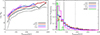 |
Fig. 2. Left panel: Stellar halo mass as a function of the transition radius Rtrans at different redshifts, as indicated in the legend. The two dashed black lines represent the 16th and 84th percentiles of the distribution at z = 0. Right panel: Distribution of transition radii at different redshifts (different colors) and as inferred from observations (VEGAS, green line). The model distributions extend to systematically higher values of Rtrans than the observational one, while the VEGAS distribution is more narrowly peaked at smaller radii (see the vertical lines indicating medians, 16th and 84th percentiles of the distributions for the model predictions at z = 0 (black) and VEGAS (green)). This offset reflects the different definitions adopted in the SAM and in observations, as well as differences in sample selection. The comparison should therefore be interpreted in a statistical sense, focusing on typical scales and trends rather than on a one-to-one correspondence. Across all redshifts, the majority of model transition radii lie within ∼100 kpc, with a tail extending to higher values in the most massive systems. |
Interestingly, at fixed Rtrans, the SH mass increases with redshift. A constant transition radius implies the same ICL concentration and a halo concentration that is lower by a factor γ (between 1 and 3; see Section 2). Given the relation of halo mass to concentration (e.g., Prada et al. 2012; Correa et al. 2015; Child et al. 2018), this suggests that BCG host halos at different epochs might exhibit similar concentrations within the intrinsic scatter of the relation. At higher redshift, these concentrations correspond to dynamically more evolved halos, which likely produced a substantial amount of ICL, part of which is converted into significant SH mass. We verified this scenario by selecting samples of halos at z = 2 and comparing them with their z = 0 counterparts at fixed Rtrans. This trend is indeed statistically robust.
Another point worth stressing is that Rtrans can extend to very large scales: at z = 0, it can reach ∼400 kpc in the most massive halos, it reaches ∼300 kpc at z = 1, and at z = 2, it still extends to ∼150 kpc. The systematic decrease in Rtrans with redshift is a natural outcome of the hierarchical growth of structures: halos at higher redshifts are less massive on average and dynamically younger. At least at z = 0, where a comparison is possible, our results agree well with those of Proctor et al. (2024), who analyzed the EAGLE (Schaye et al. 2015; Crain et al. 2015) and C-EAGLE (Bahé et al. 2017; Barnes et al. 2017) simulations using an independent definition of Rtrans (Contini et al. 2024b).
The right panel of Fig. 2 shows the distribution of transition radii, Rtrans, predicted by the model at different redshifts and inferred from the VEGAS observations. While the observational distribution is narrowly peaked at relatively small radii, the model predicts a broader distribution extending to systematically higher values, particularly at low redshift. This offset indicates that observationally defined transition radii, derived from multicomponent photometric decompositions through minimization of the rms scatter of the fits (e.g. Seigar et al. 2007), and shown to correlate with changes in surface brightness, ellipticity, position angle, and color profiles (Spavone et al. 2017, 2021), do not necessarily trace the same physical boundary as the model-defined Rtrans, which separates stars bound to the central galaxy from the diffuse intracluster component4.
Part of the difference might reflect sample selection effects, as the observational data probe a restricted range of massive systems in the local Universe, whereas the model includes central galaxies spanning a wider range of stellar and halo masses. In addition, the heterogeneous distances of the VEGAS targets introduce an additional source of scatter in the conversion from angular to physical radii. For these reasons, the comparison between observations and model predictions should be interpreted in a statistical and qualitative sense, focusing on typical scales and trends and not on a direct one-to-one correspondence.
In Figure 3 we present the scaling relations between the SH and the BCG mass (left panel), and between the SH and the ICL mass (right panel) at z = 0. In both cases, circles are color coded according to the halo concentration. The SH mass correlates with the BCG and the ICL mass, although the latter relation exhibits a significantly smaller scatter. This is expected because SHs form directly from stars belonging to the ICL or because the SH is a tail of the ICL and no separate component. An important trend visible in both panels is that the SH mass tends to increase in less concentrated halos, which are also typically the most massive ones. At first sight, this might appear to differ from the results of Contini et al. (2023), who found higher ICL fractions in more concentrated halos. However, we stress that our plots show mass-to-mass relations, not fraction-to-mass relations. Moreover, the halo concentration is directly linked to the transition radius Rtrans. Less concentrated halos (and their associated ICL) are characterized by higher values of Rtrans (see Equation (2)), which in turn implies a higher SH mass, depending on the amount of ICL already in place. The key message is therefore that halo concentration, through its connection with the ICL concentration, plays a crucial role in shaping the formation of SHs.
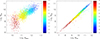 |
Fig. 3. Scaling relations between the mass of stellar halos and that of the associated central galaxy (left panel) and intracluster light (right panel). The color bar encodes the dark matter halo concentration, with redder colors corresponding to higher concentrations. The stellar halo mass correlates well with the BCG and the ICL mass, with a notably smaller scatter in the ICL case. In both relations, halo concentration plays a key role: stellar halos tend to be more massive in less concentrated dark matter halos, which are also the most massive systems. |
Another striking feature is that both scaling relations appear to be nearly linear by eye. Focusing on the SH–BCG mass relation, we performed a simple linear fit in logarithmic space. The best-fit slope is 0.99, with a relatively small intercept of −2.07, confirming that the relation is essentially linear. This allowed us to reformulate the fit in terms of the mass fraction fSH − BCG on the y-axis, since the fSH − BCG–BCG mass relation is nearly constant. Within the range of log MBCG = [9.5, 13], we obtained the following values: mean fSH − BCG = [0.0074, 0.0069], mean+1σ = [0.0158, 0.0174], mean−1σ = [0.0034, 0.0028], mean+2σ = [0.0347, 0.0427], and mean−2σ = [0.0016, 0.0011]. These predictions compare very well with the observed data from Merritt et al. (2016) (their Figure 5, left panel) and Gilhuly et al. (2022) (their Figure 7). Both works were based on the Dragonfly Survey, with Gilhuly et al. extending the analysis to lower-mass galaxies than Merritt et al. Specifically, our ±1σ region encompasses the bulk of the data by Merritt et al., with the exception of three outliers that are not even included within ±2σ. Similarly, for the sample by Gilhuly et al., our ±1σ region accounts for most of their galaxies, while ±2σ essentially covers the full set. This agreement provides strong support for the robustness of our SH implementation in FEGA25.
While the halo concentration is a fundamental driver of ICL and SH formation, another quantity that may play a role is the efficiency of ICL production. Intuitively, the larger the amount of ICL, the more likely the formation of massive SHs. We explore this aspect in Figure 4, which shows the same two relations as in Figure 3, but this time, with circles color-coded by the ICL formation efficiency. We defined the efficiency as the ratio of the total ICL mass assembled up to a given epoch (here, z = 0) and the total halo mass. As shown in Contini et al. (2024a), the efficiency of ICL formation is broadly independent of halo mass, although this does not necessarily preclude a role in SH growth.
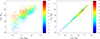 |
Fig. 4. Similar to Figure 3, the plots show the same scaling relations, but with the color bar now indicating the logarithm of the efficiency of ICL production in dark matter halos. The efficiency is defined as the ratio between the ICL mass and the halo mass. A clear trend emerges in both panels: stellar halos tend to be more massive when the efficiency of ICL production is higher. In the left panel, this appears at fixed BCG mass, where redder colors correspond to more massive stellar halos, while in the right panel the trend follows the main relation itself. |
The two panels in Figure 4 highlight a clear trend: SHs are more massive in systems with higher ICL formation efficiencies. This is most evident in the left panel, where at fixed BCG mass (and thus, at approximately fixed halo mass within a range), redder circles indicate higher efficiencies. In the SH–ICL mass plane, the trend is somewhat less pronounced, but still visible, with low-mass SHs corresponding to bluer (lower-efficiency) points, and high-mass SHs associated with redder ones. Taken together, halo concentration and ICL formation efficiency emerge as key factors in shaping SH properties. We also emphasize that a repetition of this analysis at higher redshifts led to no significant differences: the trends already hold at earlier times, with the expected variations in scatter due to number statistics.
After exploring these scaling relations, we now turn to properties that are more challenging to model in a semianalytic framework, namely colors and metallicities.
3.2. Colors and metallicity
Figure 5 shows the g − r and r − i diagram for BCGs (red), SHs (black), and ICL (blue) for each individual system in our sample as a function of redshift (different panels). There is a diversity of colors, spanning a wide range in both cases. Overall, it appears that all three components have similar colors and are independent of redshift, but all of them also progressively redden from high redshift to the present day. At z = 0, we compare our predictions with the observed SH colors from VEGAS (green diamonds for VG and brown squares for FDS). The uncertainties in the observational data are broad enough to encompass most of our predicted values, although the distribution appears to be somewhat more scattered. Nevertheless, the majority of the observed points fall within the cloud of model predictions. This is visible by eye by comparing the black triangle with error bars (indicating mean and ±1σ distribution of the predicted SH colors). At ±2σ, most of the green diamonds and error bars fall within the predicted distribution.
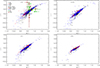 |
Fig. 5. Relation between g − r and r − i colors for the BCGs (red), stellar halos (black), ICL (blue) at different redshifts (separate panels), and as observed in VEGAS (green diamonds for VG and brown squares for FDS, at z = 0). Overall, the three components exhibit comparable colors, largely independent of redshift, and all progressively redden (shifting towards the right side of the diagrams) as the redshift approaches the present epoch. |
In order to catch any possible difference between the colors of the different components, we plot in Figure 6 their distributions at z = 0 (left panel) and z = 2 (right panel). Solid lines represent the g − r, while the dashed ones indicate r − i, and line colors denote the three components as in the previous figure. Plotted together with our predictions at z = 0, we show the mean values of the two observed colors (thick green solid and dashed lines) along with their corresponding ±1σ distributions (thin green solid and dashed lines).
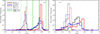 |
Fig. 6. Distributions for each component at z = 0 (left panel) and z = 2 (right panel) for the same colors as in the previous figure. As discussed above, both colors become redder with time, but the distributions reveal notable differences. At z = 0, the BCGs display narrower distributions with a more pronounced peak, while at z = 2 their distributions appear quite different. Overall, stellar halos and the ICL exhibit similar distributions at z = 0, whereas at z = 2 they are statistically distinct. Importantly, BCGs are consistently redder than the other two components, independent of redshift. The thick green lines (solid and dashed) represent the mean colors observed in VEGAS (VG+FDS), while the thinner ones indicated the ±1σ distribution. The predicted g − r and r − i of the SHs at z = 0 are very close to the observed ones. |
Several key points are worth discussing, mainly in the difference between the two redshifts we investigated. First of all, as already noted in Figure 5, both colors tend to become redder with time, which is a natural consequence of aging. For SHs and ICL, it is understandable since they lack any star formation, and aging overcomes the newly stripped stars that might be blue. For the BCGs instead, it just means that they age by passive evolution with little episodes of star formation after a period of growth due to mergers (e.g., Oliva-Altamirano et al. 2014; Lee & Yi 2017 or Contini et al. 2024c for a review), and the fact that g − r grows faster than r − i is a clear indication of this.
Another important feature of the plot is that at z = 0, all components and for both colors have narrower distributions than those at z = 2, and the peaks are more pronounced. This highlights the variety of the populations at high redshifts with respect to an old population at the present day. The distributions appear to be similar at z = 0, but this is not the case at z = 2. At this redshift, when the Universe was just 3 Gyr old, BCGs are consistently redder than the other two components. This trend is seen even at z = 0, but to a lesser degree, meaning that SHs and ICL age faster than BCGs. Again, this is understandable because no star formation occurs in these two components. More importantly, the model predictions for both colors agree very well with the observed SH colors.
To summarize, our model predicts a negative gradient in colors from the inner component, the BCG, to the outer component, the ICL, but this trend weakens over time. Moreover, there is not statistical distinction between SHs and ICL, implying that they have very similar colors at any time. Once again, this can be explained by the tight link between the components, given that SHs form directly from stars originally belonging to the ICL.
Taken together, our results indicate that broadband colors alone are insufficient to separate SHs from the surrounding ICL: the two components display virtually indistinguishable g − r and r − i distributions at all epochs, while BCGs remain only mildly redder on average by z = 0. This degeneracy is physically expected if SHs are continuously replenished by the same accreted populations that build the ICL, and it is consistent with the large object-to-object scatter in observed color gradients reported for nearby halos and extended envelopes (e.g. Merritt et al. 2016; Gilhuly et al. 2022). In the Local Group, the Milky Way and M31 show negative color/metallicity gradients in their outskirts, but with amplitudes that strongly depend on each system’s recent accretion history (Kalirai et al. 2006; Gilbert et al. 2014; Deason et al. 2014). Cosmological simulations likewise predict broadly similar colors for ex situ dominated components such as outer BCG envelopes, SHs, and ICL, which are modulated by the stochastic contribution of a few massive progenitors (Pillepich et al. 2018; Monachesi et al. 2019; Elias et al. 2020; Wright et al. 2024). Practically, our findings imply that future wide-field programs (e.g., LSST imaging combined with WEAVE/4MOST spectroscopy) should rely on chemo-dynamical tracers and not on broadband colors alone to unambiguously separate SHs from the diffuse intracluster population (Cooper et al. 2011; Helmi 2020; Spavone et al. 2020, 2021, 2022; Iodice et al. 2016).
By focusing on the metallicity of the three components, we can assess whether the trends observed for colors are also present in the metallicity distributions. In Figure 7 we plot the metallicity of the three components of each system in our sample as a function of their radius and at the usual redshifts (different panels). The colored rectangles show the 16th and 84th distribution for each component. The predictions at z = 0 are accompanied by observed SH metallicities from FDS (brown squares) only, because they are not available for VG. Before we describe the features of the plot, we explain how we calculated the radius of each component in order to place them in the plot. In the case of the BCG, its radius was defined as in Contini et al. (2019) by mass-weighting the bulge and disk radii,
 (3)
(3)
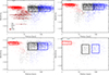 |
Fig. 7. Metallicity profiles (log Z) of the three components as a function of radius (see text for details), shown at different redshifts (separate panels). At high redshift, stellar halos and the ICL tend to be more metal-poor than the BCGs, although this trend becomes less evident at lower redshifts. The shaded rectangles mark the regions enclosing the 16th to 84th percentiles of the distributions, and the brown squares represent the observed metallicities in FDS at z = 0. |
where Rbulge and 1.68 ⋅ Rsl are the half stellar mass radii of the bulge and disk, and Mbulge*, Mdisk*, and MBCG* are the stellar masses of the bulge, disk, and BCG as a whole, respectively. SHs are defined in terms of the transition radius Rtrans; accordingly, we placed them at half this radius. Similarly, we placed FDS data at R2/2. For the ICL instead, there is no clear placement because, in principle, they can extend up to the virial radius. Considering that the real radius has no physical effect in the context of this plot, we placed the ICL at 2 ⋅ Rtrans.
The plot shows us that SHs and ICL are poorer in metals than the BCGs at high redshift, but the gap becomes smaller approaching redshift z = 0, where the difference in metallicity between the three components is indistinguishable. SHs and ICL have the same metallicity regardless of the redshift. FDS data lie within the cloud of predicted SH metallicities on the left side of the panel, closely tracing the BCG distribution. This behavior likely arises from two factors: first, the observationally defined R2 differs intrinsically from our model definition of Rtrans, although the two are physically related; second, while our analysis focused on central galaxies in the SAM, the FDS sample mainly consists of satellites, which are less massive on average than the model centrals.
As done above with colors, we need to quantify the real difference better, if there is any. We therefor plot in Figure 8 the metallicity distributions of BCGs, SHs, and ICL, at z = 0 (left panel) and z = 2 (right panel). At z = 2, while the metallicity distributions of SHs and ICL are very similar, almost identical, that of BCGs is very much different and peaks at higher metallicity. The peak for the BCGs is at ∼ − 1.7, while the peaks of SHs and ICL are wide, between ∼ − 2.0 and ∼ − 2.3 on average at −2.15. Hence, the gap in metallicity between BCGs and SH-ICL is around 0.4 dex at z = 2.
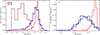 |
Fig. 8. Metallicity distributions (log Z) for BCGs (red), stellar halos (black), and ICL (blue) at z = 0 (left panel) and z = 2 (right panel), similar to Figure 6. In both panels, stellar halos and the ICL exhibit broadly comparable distributions, whereas BCGs remain systematically more metal-rich than the other two components, regardless of redshift. The separation is present at all epochs, but appears much more pronounced at z = 2. The brown line at z = 0 represents the observed distribution in FDS (SHs). |
At z = 0, the picture is rather different. The three distributions are very similar, although those of SHs and ICL are wider. The average metallicity of BCGs at the peaks does not change with respect to that at z = 2 (∼ − 1.7), but SHs and ICL eventually become more metal rich and almost reach the average metallicity of BCGs. The gap between the mean metallicity of BCGs and that of SHs-ICL is around 0.1 dex. As noted above (and therefore expected), the FDS SH metallicity distribution peaks at systematically lower values than our predictions, suggesting that these SHs likely originate from disrupted dwarf galaxies, as noted in Section 1.
To summarize, similarly to colors, our model predicts a negative gradient from the BCG to the ICL, which is very clear at high redshifts, but almost flattens over time. Again, as for the colors, SH and ICL have the same metallicity.
The redshift evolution of the metallicity strengthens the above picture. At z = 2, the offset is ≃0.4 dex between BCGs and the SH–ICL pair, with the latter two being essentially indistinguishable; by z = 0, the gap shrinks to ≃0.1 dex as SHs and the ICL become richer in metals. This convergence naturally arises if late-time growth in the outskirts is increasingly driven by the stripping of relatively massive chemically evolved satellites, while early assembly is dominated by lower-mass metal-poor dwarfs. The trend echoes simulation results in which ex situ accretion builds extended BCG envelopes at late times and predicts shallow, slowly evolving outer metallicity gradients (Nelson et al. 2024; Montenegro-Taborda et al. 2023; Contreras-Santos et al. 2024; Pillepich et al. 2018). Conversely, the systematically lower metallicities measured in our observed samples are consistent with a larger fractional contribution from disrupted dwarfs (e.g. Mouhcine et al. 2005; Harmsen et al. 2017; D’Souza & Bell 2018; Spavone et al. 2017; Ragusa et al. 2021, 2022), which might reflect environmental or selection differences with respect to our central-galaxy sample. In this context, the average metallicity of SHs/ICL is a sensitive diagnostic of the mass spectrum of destroyed progenitors; the combination of metallicity with α–enhancement and kinematics is expected to further distinguish rapid early enrichment from extended low-mass accretion histories (Venn et al. 2004; Deason et al. 2016).
4. Conclusions
We have investigated the properties of stellar halos (SHs) of bright central galaxies (BCGs), building on our previous implementation of SH formation in the semianalytic model FEGA25 and extending the analysis to their redshift evolution in terms of scaling relations, colors, and metallicities. Our main findings are summarized below.
4.1. 1. Scaling with halo structure.
The SH mass correlates tightly with the BCG and intracluster light (ICL) masses. While these two relations are basically linear, the SH–ICL relation exhibits significantly smaller scatter, as expected from the adopted SH definition, consistent with the direct origin of SHs from ICL stars. The halo concentration emerges as a fundamental driver: less concentrated (typically, more massive) halos host more extended transition radii and correspondingly larger SHs. In addition, SHs are more massive in systems with a higher ICL formation efficiency, showing that structural and baryonic processes shape the SH–ICL connection. We note that the residual scatter in these relations reflects variations in the halo concentration, ICL assembly histories, and the physically motivated stability criteria applied in the model.
4.2. 2. Transition radii.
The distribution of Rtrans predicted by the model peaks around 30−40 kpc, nearly regardless of redshift, with ∼90% of systems below 100 kpc. However, massive halos can reach Rtrans ∼ 400 kpc at z = 0. The weak redshift evolution suggests that SH sizes are largely set by the halo concentration and not by epoch, in agreement with recent simulation-based determinations (e.g., Proctor et al. 2024). At the same time, the observational Rtrans distribution inferred from VEGAS is more narrowly peaked at smaller radii, indicating an offset with respect to the model predictions. This difference reflects the distinct definitions adopted in observations and in the semianalytic model, as well as sample-selection effects. The comparison should therefore be interpreted in a statistical and qualitative sense and not as a direct one-to-one correspondence between individual systems.
4.3. 3. Colors.
All three components (BCGs, SHs, and ICL) progressively redden with cosmic time. By z = 0, their color distributions largely overlap, with only a mild offset that leaves BCGs redder on average. SHs and ICL are virtually indistinguishable in broadband colors at all epochs, implying that colors alone are not sufficient to separate these two components observationally. This degeneracy reinforces the idea of a common physical origin and is consistent with the large scatter of observed color gradients in nearby halos. In the model, colors were derived self-consistently from the star-formation histories of the different stellar components and were not treated as free parameters.
4.4. 4. Metallicities.
At z = 2, BCGs are richer in metals than either SHs or ICL by ∼0.4 dex, but this gap shrinks to ∼0.1 dex by z = 0 as SHs/ICL become progressively more enriched through the stripping of more massive satellites. The convergence of metallicities over time highlights the role of late accretion in building chemically evolved outskirts. FDS observations, however, peak at lower metallicities, suggesting that disrupted dwarf galaxies contribute more strongly to observed halos than in our central-galaxy sample. This indicates possible environmental or selection effects and emphasizes the diagnostic power of metallicity gradients for constraining progenitor mass functions.
4.5. 5. Overall picture.
The SHs appear to be transition regions between the stars bound to BCGs and those belonging to the diffuse ICL. We emphasize that this interpretation follows directly from the adopted SH definition, while the trends in mass, structure, and stellar populations we discussed reflect genuine physical dependences on halo concentration, ICL formation efficiency, and the mass spectrum of accreted satellites. These conclusions support a view in which SHs are not isolated components, but are the inner manifestation of the ICL, dynamically and chemically coupled to the outer galaxy environment. Future wide-field imaging and spectroscopic surveys (e.g., LSST, WEAVE, and 4MOST) will be crucial for testing these predictions by simultaneously probing structure, metallicity, and kinematics in large samples of halos in diverse environments.
Acknowledgments
The authors thank the anonymous referee for their constructive comments, which have significantly contributed to improving this manuscript. E.C. and S.K.Y. acknowledge support from the Korean National Research Foundation (RS-2025-00514475; RS-2022-NR070872), and E.C. acknowledges support from the Korean National Research Foundation (RS-2023-00241934). M.S. and E.I. acknowledge the support by the Italian Ministry for 1224 Education University and Research (MIUR) grant PRIN 2022 2022383WFT 1225 “SUNRISE”, CUP C53D23000850006 and by VST funds. R.R. acknowledges financial support through grants PRIN-MIUR 2020SKSTHZ and through INAF-WEAVE StePS funds.
References
- Amorisco, N. C. 2017, MNRAS, 464, 2882 [Google Scholar]
- Bahé, Y. M., Barnes, D. J., Dalla Vecchia, C., et al. 2017, MNRAS, 470, 4186 [Google Scholar]
- Barnes, D. J., Kay, S. T., Bahé, Y. M., et al. 2017, MNRAS, 471, 1088 [Google Scholar]
- Beers, T. C., Carollo, D., Ivezić, Ž., et al. 2012, ApJ, 746, 34 [NASA ADS] [CrossRef] [Google Scholar]
- Belokurov, V., Erkal, D., Evans, N. W., Koposov, S. E., & Deason, A. J. 2018, MNRAS, 478, 611 [Google Scholar]
- Belokurov, V., Sanders, J. L., Fattahi, A., et al. 2020, MNRAS, 494, 3880 [Google Scholar]
- Beltrand, C., Monachesi, A., D’Souza, R., et al. 2024, A&A, 690, A115 [NASA ADS] [CrossRef] [EDP Sciences] [Google Scholar]
- Bullock, J. S., & Johnston, K. V. 2005, ApJ, 635, 931 [Google Scholar]
- Capaccioli, M., Spavone, M., Grado, A., et al. 2015, A&A, 581, A10 [NASA ADS] [CrossRef] [EDP Sciences] [Google Scholar]
- Carollo, D., Beers, T. C., Lee, Y. S., et al. 2007, Nature, 450, 1020 [NASA ADS] [CrossRef] [Google Scholar]
- Carollo, D., Beers, T. C., Chiba, M., et al. 2010, ApJ, 712, 692 [NASA ADS] [CrossRef] [Google Scholar]
- Chabrier, G. 2003, PASP, 115, 763 [Google Scholar]
- Child, H. L., Habib, S., Heitmann, K., et al. 2018, ApJ, 859, 55 [NASA ADS] [CrossRef] [Google Scholar]
- Contini, E., & Gu, Q. 2020, ApJ, 901, 128 [NASA ADS] [CrossRef] [Google Scholar]
- Contini, E., De Lucia, G., Villalobos, Á., & Borgani, S. 2014, MNRAS, 437, 3787 [Google Scholar]
- Contini, E., Yi, S. K., & Kang, X. 2018, MNRAS, 479, 932 [NASA ADS] [Google Scholar]
- Contini, E., Yi, S. K., & Kang, X. 2019, ApJ, 871, 24 [Google Scholar]
- Contini, E., Jeon, S., Rhee, J., Han, S., & Yi, S. K. 2023, ApJ, 958, 72 [NASA ADS] [CrossRef] [Google Scholar]
- Contini, E., Rhee, J., Han, S., Jeon, S., & Yi, S. K. 2024a, AJ, 167, 7 [NASA ADS] [CrossRef] [Google Scholar]
- Contini, E., Spavone, M., Ragusa, R., Iodice, E., & Yi, S. K. 2024b, A&A, 692, L9 [NASA ADS] [CrossRef] [EDP Sciences] [Google Scholar]
- Contini, E., Yi, S. K., & Jeon, S. 2024c, ArXiv e-prints [arXiv:2404.01560] [Google Scholar]
- Contini, E., Yi, S. K., Jeon, S., & Rhee, J. 2024d, ApJS, 274, 41 [NASA ADS] [CrossRef] [Google Scholar]
- Contini, E., Seo, C., Rhee, J., Jeon, S., & Yi, S. K. 2025a, ApJS, 281, 2 [Google Scholar]
- Contini, E., Yi, S. K., Rhee, J., & Jeon, S. 2025b, ApJS, 279, 18 [Google Scholar]
- Contreras-Santos, A., Knebe, A., Cui, W., et al. 2024, A&A, 683, A59 [NASA ADS] [CrossRef] [EDP Sciences] [Google Scholar]
- Cooper, A. P., Cole, S., Frenk, C. S., et al. 2010, MNRAS, 406, 744 [Google Scholar]
- Cooper, A. P., Martínez-Delgado, D., Helly, J., et al. 2011, ApJ, 743, L21 [NASA ADS] [CrossRef] [Google Scholar]
- Cooper, A. P., Parry, O. H., Lowing, B., Cole, S., & Frenk, C. 2015, MNRAS, 454, 3185 [Google Scholar]
- Correa, C. A., Wyithe, J. S. B., Schaye, J., & Duffy, A. R. 2015, MNRAS, 452, 1217 [CrossRef] [Google Scholar]
- Crain, R. A., Schaye, J., Bower, R. G., et al. 2015, MNRAS, 450, 1937 [NASA ADS] [CrossRef] [Google Scholar]
- Cui, W., Knebe, A., Yepes, G., et al. 2018, MNRAS, 480, 2898 [Google Scholar]
- de Jong, R. S., Agertz, O., Berbel, A. A., et al. 2019, The Messenger, 175, 3 [NASA ADS] [Google Scholar]
- de Vaucouleurs, G. 1959, Handbuch der Physik, 53, 275 [Google Scholar]
- Deason, A. J., Belokurov, V., & Evans, N. W. 2013, ApJ, 763, 113 [Google Scholar]
- Deason, A. J., Belokurov, V., Koposov, S. E., & Rockosi, C. M. 2014, ApJ, 787, 30 [NASA ADS] [CrossRef] [Google Scholar]
- Deason, A. J., Mao, Y.-Y., & Wechsler, R. H. 2016, ApJ, 821, 5 [NASA ADS] [CrossRef] [Google Scholar]
- Drinkwater, M. J., Gregg, M. D., & Colless, M. 2001, ApJ, 548, L139 [Google Scholar]
- D’Souza, R., & Bell, E. F. 2018, MNRAS, 474, 5300 [CrossRef] [Google Scholar]
- Duc, P.-A., Cuillandre, J.-C., Karabal, E., et al. 2015, MNRAS, 446, 120 [Google Scholar]
- Efron, B. 1979, Ann. Stat., 7, 1 [Google Scholar]
- Elias, L. M., Sales, L. V., Helmi, A., & Hernquist, L. 2020, MNRAS, 495, 29 [NASA ADS] [CrossRef] [Google Scholar]
- Font, A. S., McCarthy, I. G., Crain, R. A., et al. 2011, MNRAS, 416, 2802 [NASA ADS] [CrossRef] [Google Scholar]
- Gallart, C., Bernard, E. J., Brook, C. B., et al. 2019, Nat. Astron., 3, 932 [NASA ADS] [CrossRef] [Google Scholar]
- Gendron, V., & Martel, H. 2025, MNRAS, 541, 2513 [Google Scholar]
- Gilbert, K. M., Kalirai, J. S., Guhathakurta, P., et al. 2014, ApJ, 796, 76 [NASA ADS] [CrossRef] [Google Scholar]
- Gilhuly, C., Merritt, A., Abraham, R., et al. 2022, ApJ, 932, 44 [NASA ADS] [CrossRef] [Google Scholar]
- Grand, R. J. J., Gómez, F. A., Marinacci, F., et al. 2017, MNRAS, 467, 179 [NASA ADS] [Google Scholar]
- Guo, Q., White, S., Boylan-Kolchin, M., et al. 2011, MNRAS, 413, 101 [Google Scholar]
- Harmsen, B., Monachesi, A., Bell, E. F., et al. 2017, MNRAS, 466, 1491 [Google Scholar]
- Helmi, A. 2008, A&ARv, 15, 145 [CrossRef] [Google Scholar]
- Helmi, A. 2020, ARA&A, 58, 205 [Google Scholar]
- Helmi, A., Babusiaux, C., Koppelman, H. H., et al. 2018, Nature, 563, 85 [Google Scholar]
- Hopkins, P. F., Kereš, D., Oñorbe, J., et al. 2014, MNRAS, 445, 581 [NASA ADS] [CrossRef] [Google Scholar]
- Ibata, R. A., Lewis, G. F., McConnachie, A. W., et al. 2014, ApJ, 780, 128 [Google Scholar]
- Iodice, E., Capaccioli, M., Grado, A., et al. 2016, ApJ, 820, 42 [Google Scholar]
- Iodice, E., Spavone, M., Cantiello, M., et al. 2017, ApJ, 851, 75 [Google Scholar]
- Iodice, E., Spavone, M., Capaccioli, M., et al. 2019, A&A, 623, A1 [NASA ADS] [CrossRef] [EDP Sciences] [Google Scholar]
- Iodice, E., Spavone, M., Capaccioli, M., et al. 2021, The Messenger, 183, 25 [NASA ADS] [Google Scholar]
- Ivezić, Ž., Kahn, S. M., Tyson, J. A., et al. 2019, ApJ, 873, 111 [Google Scholar]
- Jin, S., Trager, S. C., Dalton, G. B., et al. 2024, MNRAS, 530, 2688 [NASA ADS] [CrossRef] [Google Scholar]
- Joo, H., Jee, M. J., Kim, J., et al. 2025, ApJ, 990, 96 [Google Scholar]
- Kalirai, J. S., Gilbert, K. M., Guhathakurta, P., et al. 2006, ApJ, 648, 389 [Google Scholar]
- Krajnović, D., Emsellem, E., den Brok, M., et al. 2018, MNRAS, 477, 5327 [Google Scholar]
- Lane, J. M. M., Bovy, J., & Mackereth, J. T. 2022, MNRAS, 510, 5119 [NASA ADS] [CrossRef] [Google Scholar]
- Lee, J., & Yi, S. K. 2017, ApJ, 836, 161 [Google Scholar]
- Merritt, A., van Dokkum, P., Abraham, R., & Zhang, J. 2016, ApJ, 830, 62 [Google Scholar]
- Mihos, J. C., Harding, P., Feldmeier, J. J., et al. 2017, ApJ, 834, 16 [Google Scholar]
- Monachesi, A., Gómez, F. A., Grand, R. J. J., et al. 2016, MNRAS, 459, L46 [NASA ADS] [CrossRef] [Google Scholar]
- Monachesi, A., Gómez, F. A., Grand, R. J. J., et al. 2019, MNRAS, 485, 2589 [NASA ADS] [CrossRef] [Google Scholar]
- Montenegro-Taborda, D., Rodriguez-Gomez, V., Pillepich, A., et al. 2023, MNRAS, 521, 800 [NASA ADS] [CrossRef] [Google Scholar]
- Montes, M., & Trujillo, I. 2018, MNRAS, 474, 917 [Google Scholar]
- Mouhcine, M., Ferguson, H. C., Rich, R. M., Brown, T. M., & Smith, T. E. 2005, ApJ, 633, 810 [NASA ADS] [CrossRef] [Google Scholar]
- Naidu, R. P., Conroy, C., Bonaca, A., et al. 2020, ApJ, 901, 48 [Google Scholar]
- Navarro, J. F., Frenk, C. S., & White, S. D. M. 1997, ApJ, 490, 493 [Google Scholar]
- Nelson, D., Pillepich, A., Springel, V., et al. 2018, MNRAS, 475, 624 [Google Scholar]
- Nelson, D., Springel, V., Pillepich, A., et al. 2019, Comput. Astrophys. Cosmol., 6, 2 [Google Scholar]
- Nelson, D., Pillepich, A., Ayromlou, M., et al. 2024, A&A, 686, A157 [NASA ADS] [CrossRef] [EDP Sciences] [Google Scholar]
- Oliva-Altamirano, P., Brough, S., Lidman, C., et al. 2014, MNRAS, 440, 762 [NASA ADS] [CrossRef] [Google Scholar]
- Pillepich, A., Nelson, D., Hernquist, L., et al. 2018, MNRAS, 475, 648 [Google Scholar]
- Pinna, F., Walo-Martín, D., Grand, R. J. J., et al. 2024, A&A, 683, A236 [NASA ADS] [CrossRef] [EDP Sciences] [Google Scholar]
- Planck Collaboration VI. 2020, A&A, 641, A6 [NASA ADS] [CrossRef] [EDP Sciences] [Google Scholar]
- Prada, F., Klypin, A. A., Cuesta, A. J., Betancort-Rijo, J. E., & Primack, J. 2012, MNRAS, 423, 3018 [NASA ADS] [CrossRef] [Google Scholar]
- Proctor, K. L., Lagos, C. D. P., Ludlow, A. D., & Robotham, A. S. G. 2024, MNRAS, 527, 2624 [Google Scholar]
- Ragusa, R., Spavone, M., Iodice, E., et al. 2021, A&A, 651, A39 [NASA ADS] [CrossRef] [EDP Sciences] [Google Scholar]
- Ragusa, R., Mirabile, M., Spavone, M., et al. 2022, Front. Astron. Space Sci., 9, 852810 [CrossRef] [Google Scholar]
- Ragusa, R., Iodice, E., Spavone, M., et al. 2023, A&A, 670, L20 [NASA ADS] [CrossRef] [EDP Sciences] [Google Scholar]
- Sarzi, M., Iodice, E., Coccato, L., et al. 2018, A&A, 616, A121 [NASA ADS] [CrossRef] [EDP Sciences] [Google Scholar]
- Schaye, J., Crain, R. A., Bower, R. G., et al. 2015, MNRAS, 446, 521 [Google Scholar]
- Seigar, M. S., Graham, A. W., & Jerjen, H. 2007, MNRAS, 378, 1575 [Google Scholar]
- Spavone, M., Capaccioli, M., Napolitano, N. R., et al. 2017, A&A, 603, A38 [NASA ADS] [CrossRef] [EDP Sciences] [Google Scholar]
- Spavone, M., Iodice, E., Capaccioli, M., et al. 2018, ApJ, 864, 149 [Google Scholar]
- Spavone, M., Iodice, E., van de Ven, G., et al. 2020, A&A, 639, A14 [NASA ADS] [CrossRef] [EDP Sciences] [Google Scholar]
- Spavone, M., Krajnović, D., Emsellem, E., Iodice, E., & den Brok, M. 2021, A&A, 649, A161 [NASA ADS] [CrossRef] [EDP Sciences] [Google Scholar]
- Spavone, M., Iodice, E., D’Ago, G., et al. 2022, A&A, 663, A135 [NASA ADS] [CrossRef] [EDP Sciences] [Google Scholar]
- Spavone, M., Iodice, E., Lohmann, F. S., et al. 2024, A&A, 689, A306 [NASA ADS] [CrossRef] [EDP Sciences] [Google Scholar]
- Springel, V., Pakmor, R., Zier, O., & Reinecke, M. 2021, MNRAS, 506, 2871 [NASA ADS] [CrossRef] [Google Scholar]
- Venhola, A., Peletier, R., Laurikainen, E., et al. 2017, A&A, 608, A142 [NASA ADS] [CrossRef] [EDP Sciences] [Google Scholar]
- Venhola, A., Peletier, R., Laurikainen, E., et al. 2018, A&A, 620, A165 [NASA ADS] [CrossRef] [EDP Sciences] [Google Scholar]
- Venn, K. A., Irwin, M., Shetrone, M. D., et al. 2004, AJ, 128, 1177 [NASA ADS] [CrossRef] [Google Scholar]
- Wright, A. C., Tumlinson, J., Peeples, M. S., et al. 2024, ApJ, 970, 70 [NASA ADS] [CrossRef] [Google Scholar]
Bulge and disk formation and evolution are implemented in FEGA as done in Guo et al. (2011).
Within the semianalytic framework adopted here, the gravitational softening length does not directly affect the predicted galaxy structural properties, which are computed analytically rather than resolved numerically. To further minimize resolution-driven effects, each simulation was therefore used only within the halo-mass regime where it provides a reliable sampling of the underlying population, and no direct comparison of the same systems across different resolutions is performed in this work.
The adoption of a power-law relation between R1 and R2 was motivated by the fact that both quantities trace characteristic transition scales in multicomponent surface brightness profiles and are therefore expected to scale approximately proportionally in logarithmic space.
For the observational comparison shown in Figure 2, we used the R2 values derived from VEGAS, corresponding to the transition between the accreted bound and the diffuse unbound stellar components.
Appendix A: Resolution tests
We assess the impact of numerical resolution on the main scaling relations discussed in this work by comparing results obtained from simulations with different mass resolutions over the stellar-mass ranges where they overlap. In particular, we analyse the relations between SH mass and transition radius, SH mass and BCG stellar mass, and SH mass and ICL mass.
Figure A.1 shows the relation between SH mass and Rtrans for the different simulations. The median trends and scatter are consistent within the overlapping mass ranges, with no systematic offsets as a function of resolution. Similarly, Figure A.2 compares the SH–BCG and SH–ICL mass relations, which also display fully consistent behaviour across simulations of different resolution.
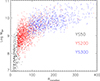 |
Fig. A.1. Relation between SH mass and transition radius Rtrans for simulations with different mass resolutions: YS50 (black), YS200 (red), and YS300 (blue). The relations are shown over the stellar-mass ranges covered by each of them. The median trends are consistent within the scatter, with no systematic dependence on numerical resolution, indicating that the SH–Rtrans relation is robust against resolution effects. |
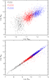 |
Fig. A.2. Scaling relations between SH mass and BCG stellar mass (upper panel), and SH mass and ICL mass (bottom panel), for simulations with different mass resolutions: YS50 (black), YS200 (red), and YS300 (blue). The agreement between the median relations in the overlapping mass ranges demonstrates that the main scaling relations discussed in the paper are not driven by numerical resolution. |
These tests indicate that the scaling relations presented in the main text are not driven by numerical resolution effects. This result is expected, as the semianalytic model traces integrated stellar components whose global properties primarily depend on halo assembly histories rather than on the detailed resolution of individual substructures.
We therefore conclude that numerical resolution does not significantly affect the trends discussed in this work. For this reason, additional properties such as colors and metallicities, which are derived from the same integrated stellar populations, are not expected to show a stronger dependence on resolution.
All Tables
All Figures
|
Fig. 1. Schematic representation of central galaxies and their surrounding stellar halos and intracluster stars. The stellar halo is defined as the stellar component within the transition radius Rtrans, marking the intermediate region between the galaxy and the intracluster light. |
| In the text | |
|
Fig. 2. Left panel: Stellar halo mass as a function of the transition radius Rtrans at different redshifts, as indicated in the legend. The two dashed black lines represent the 16th and 84th percentiles of the distribution at z = 0. Right panel: Distribution of transition radii at different redshifts (different colors) and as inferred from observations (VEGAS, green line). The model distributions extend to systematically higher values of Rtrans than the observational one, while the VEGAS distribution is more narrowly peaked at smaller radii (see the vertical lines indicating medians, 16th and 84th percentiles of the distributions for the model predictions at z = 0 (black) and VEGAS (green)). This offset reflects the different definitions adopted in the SAM and in observations, as well as differences in sample selection. The comparison should therefore be interpreted in a statistical sense, focusing on typical scales and trends rather than on a one-to-one correspondence. Across all redshifts, the majority of model transition radii lie within ∼100 kpc, with a tail extending to higher values in the most massive systems. |
| In the text | |
|
Fig. 3. Scaling relations between the mass of stellar halos and that of the associated central galaxy (left panel) and intracluster light (right panel). The color bar encodes the dark matter halo concentration, with redder colors corresponding to higher concentrations. The stellar halo mass correlates well with the BCG and the ICL mass, with a notably smaller scatter in the ICL case. In both relations, halo concentration plays a key role: stellar halos tend to be more massive in less concentrated dark matter halos, which are also the most massive systems. |
| In the text | |
|
Fig. 4. Similar to Figure 3, the plots show the same scaling relations, but with the color bar now indicating the logarithm of the efficiency of ICL production in dark matter halos. The efficiency is defined as the ratio between the ICL mass and the halo mass. A clear trend emerges in both panels: stellar halos tend to be more massive when the efficiency of ICL production is higher. In the left panel, this appears at fixed BCG mass, where redder colors correspond to more massive stellar halos, while in the right panel the trend follows the main relation itself. |
| In the text | |
|
Fig. 5. Relation between g − r and r − i colors for the BCGs (red), stellar halos (black), ICL (blue) at different redshifts (separate panels), and as observed in VEGAS (green diamonds for VG and brown squares for FDS, at z = 0). Overall, the three components exhibit comparable colors, largely independent of redshift, and all progressively redden (shifting towards the right side of the diagrams) as the redshift approaches the present epoch. |
| In the text | |
|
Fig. 6. Distributions for each component at z = 0 (left panel) and z = 2 (right panel) for the same colors as in the previous figure. As discussed above, both colors become redder with time, but the distributions reveal notable differences. At z = 0, the BCGs display narrower distributions with a more pronounced peak, while at z = 2 their distributions appear quite different. Overall, stellar halos and the ICL exhibit similar distributions at z = 0, whereas at z = 2 they are statistically distinct. Importantly, BCGs are consistently redder than the other two components, independent of redshift. The thick green lines (solid and dashed) represent the mean colors observed in VEGAS (VG+FDS), while the thinner ones indicated the ±1σ distribution. The predicted g − r and r − i of the SHs at z = 0 are very close to the observed ones. |
| In the text | |
|
Fig. 7. Metallicity profiles (log Z) of the three components as a function of radius (see text for details), shown at different redshifts (separate panels). At high redshift, stellar halos and the ICL tend to be more metal-poor than the BCGs, although this trend becomes less evident at lower redshifts. The shaded rectangles mark the regions enclosing the 16th to 84th percentiles of the distributions, and the brown squares represent the observed metallicities in FDS at z = 0. |
| In the text | |
|
Fig. 8. Metallicity distributions (log Z) for BCGs (red), stellar halos (black), and ICL (blue) at z = 0 (left panel) and z = 2 (right panel), similar to Figure 6. In both panels, stellar halos and the ICL exhibit broadly comparable distributions, whereas BCGs remain systematically more metal-rich than the other two components, regardless of redshift. The separation is present at all epochs, but appears much more pronounced at z = 2. The brown line at z = 0 represents the observed distribution in FDS (SHs). |
| In the text | |
|
Fig. A.1. Relation between SH mass and transition radius Rtrans for simulations with different mass resolutions: YS50 (black), YS200 (red), and YS300 (blue). The relations are shown over the stellar-mass ranges covered by each of them. The median trends are consistent within the scatter, with no systematic dependence on numerical resolution, indicating that the SH–Rtrans relation is robust against resolution effects. |
| In the text | |
|
Fig. A.2. Scaling relations between SH mass and BCG stellar mass (upper panel), and SH mass and ICL mass (bottom panel), for simulations with different mass resolutions: YS50 (black), YS200 (red), and YS300 (blue). The agreement between the median relations in the overlapping mass ranges demonstrates that the main scaling relations discussed in the paper are not driven by numerical resolution. |
| In the text | |
Current usage metrics show cumulative count of Article Views (full-text article views including HTML views, PDF and ePub downloads, according to the available data) and Abstracts Views on Vision4Press platform.
Data correspond to usage on the plateform after 2015. The current usage metrics is available 48-96 hours after online publication and is updated daily on week days.
Initial download of the metrics may take a while.